Tutorial 9.6b - Factorial ANOVA (Bayesian)
14 Jan 2014
Overview
Factorial designs are an extension of single factor ANOVA designs in which additional factors are added such that each level of one factor is applied to all levels of the other factor(s) and these combinations are replicated.
For example, we might design an experiment in which the effects of temperature (high vs low) and fertilizer (added vs not added) on the growth rate of seedlings are investigated by growing seedlings under the different temperature and fertilizer combinations.
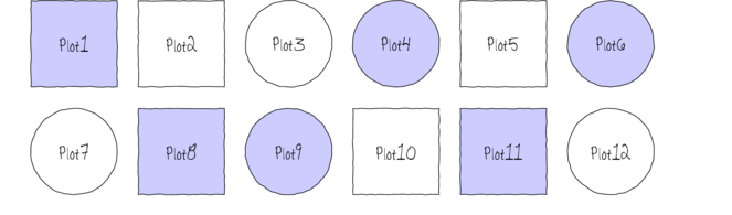
The following diagram depicts a very simple factorial design in which there are two factors (Shape and Color) each with two levels (Shape: square and circle; Color: blue and white) and each combination has 3 replicates.
In addition to investigating the impacts of the main factors, factorial designs allow us to investigate whether the effects of one factor are consistent across levels of another factor. For example, is the effect of temperature on growth rate the same for both fertilized and unfertilized seedlings and similarly, does the impact of fertilizer treatment depend on the temperature under which the seedlings are grown?
Arguably, these interactions give more sophisticated insights into the dynamics of the system we are investigating. Hence, we could add additional main effects, such as soil pH, amount of water etc along with all the two way (temp:fert, temp:pH, temp:water, etc), three-way (temp:fert:pH, temp:pH:water), four-way etc interactions in order to explore how these various factors interact with one another to effect the response.
However, the more interactions, the more complex the model becomes to specify, compute and interpret - not to mention the rate at which the number of required observations increases.
To appreciate the interpretation of interactions, consider the following figure that depicts fictitious two factor (temperature and fertilizer) designs.

It is clear from the top-right figure that whether or not there is an observed effect of adding fertilizer or not depends on whether we are focused on seedlings growth under high or low temperatures. Fertilizer is only important for seedlings grown under high temperatures. In this case, it is not possible to simply state that there is an effect of fertilizer as it depends on the level of temperature. Similarly, the magnitude of the effect of temperature depends on whether fertilizer has been added or not.
Such interactions are represented by plots in which lines either intersect or converge. The top-right and bottom-left figures both depict parallel lines which are indicative of no interaction. That is, the effects of temperature are similar for both fertilizer added and controls and vice verse. Whilst the former displays an effect of both fertilizer and temperature, the latter only fertilizer is important.
Finally, the bottom-right figure represents a strong interaction that would mask the main effects of temperature and fertilizer (since the nature of the effect of temperature is very different for the different fertilizer treatments and visa verse).
In a frequentist framework, factorial designs can consist:
- entirely of crossed fixed factors (Model I ANOVA - most common) in which conclusions are restricted to the specific combinations of levels selected for the experiment,
- entirely of crossed random factors (Model II ANOVA) or
- a mixture of crossed fixed and random factors (Model III ANOVA).
The tutorial on frequentist factorial ANOVA described procedures used to further investigate models in the presence of significant interactions as well as the complications that arise with linear models fitted to unbalanced designs. Again, these issues largely evaporate in a Bayesian framework. Consequently, we will not really dwell on these complications in this tutorial. At most, we will model some unbalanced data, yet it should be noted that we will not need to make any special adjustments in order to do so.
Linear model
The generic linear model is presented here purely for revisory purposes. If, it is unfamiliar to you or you are unsure about what parameters are to be estimated and tested, you are strongly advised to review the the tutorial on frequentist factorial ANOVA
The linear models for two and three factor design are: $$y_{ijk}=\mu+\alpha_i + \beta_{j} + (\alpha\beta)_{ij} + \varepsilon_{ijk}$$ $$y_{ijkl}=\mu+\alpha_i + \beta_{j} + \gamma_{k} + (\alpha\beta)_{ij} + (\alpha\gamma)_{ik} + (\beta\gamma)_{jk} + (\alpha\beta\gamma)_{ijk} + \varepsilon_{ijkl}$$ where $\mu$ is the overall mean, $\alpha$ is the effect of Factor A, $\beta$ is the effect of Factor B, $\gamma$ is the effect of Factor C and $\varepsilon$ is the random unexplained or residual component.
Scenario and Data
Imagine we has designed an experiment in which we had measured the response ($y$) under a combination of two different potential influences (Factor A: levels $a1$ and $a2$; and Factor B: levels $b1$, $b2$ and $b3$), each combination replicated 10 times ($n=10$). As this section is mainly about the generation of artificial data (and not specifically about what to do with the data), understanding the actual details are optional and can be safely skipped. Consequently, I have folded (toggled) this section away.
- the sample size per treatment=10
- factor A with 2 levels
- factor B with 3 levels
- the 6 effects parameters are 40, 15, 5, 0, -15,10 ($\mu_{a1b1}=40$, $\mu_{a2b1}=40+15=55$, $\mu_{a1b2}=40+5=45$, $\mu_{a1b3}=40+0=40$, $\mu_{a2b2}=40+15+5-15=45$ and $\mu_{a2b3}=40+15+0+10=65$)
- the data are drawn from normal distributions with a mean of 0 and standard deviation of 3 ($\sigma^2=9$)
> set.seed(1)
> nA <- 2  #number of levels of A
> nB <- 3  #number of levels of B
> nsample <- 10  #number of reps in each
> A <- gl(nA, 1, nA, lab = paste("a", 1:nA, sep = ""))
> B <- gl(nB, 1, nB, lab = paste("b", 1:nB, sep = ""))
> data <- expand.grid(A = A, B = B, n = 1:nsample)
> X <- model.matrix(~A * B, data = data)
> eff <- c(40, 15, 5, 0, -15, 10)
> sigma <- 3  #residual standard deviation
> n <- nrow(data)
> eps <- rnorm(n, 0, sigma)  #residuals
> data$y <- as.numeric(X %*% eff + eps)
> head(data)  #print out the first six rows of the data set
   A  B n     y
1 a1 b1 1 38.12
2 a2 b1 1 55.55
3 a1 b2 1 42.49
4 a2 b2 1 49.79
5 a1 b3 1 40.99
6 a2 b3 1 62.54
> with(data, interaction.plot(A, B, y))

>
> ## ALTERNATIVELY, we could supply the population means and get the effect parameters from these.  To
> ## correspond to the model matrix, enter the population means in the order of: a1b1, a2b1, a1b1,
> ## a2b2,a1b3,a2b3
> pop.means <- as.matrix(c(40, 55, 45, 45, 40, 65), byrow = F)
> ## Generate a minimum model matrix for the effects
> XX <- model.matrix(~A * B, expand.grid(A = factor(1:2), B = factor(1:3)))
> ## Use the solve() function to solve what are effectively simultaneous equations
> (eff <- as.vector(solve(XX, pop.means)))
[1] 40 15 5 0 -15 10
> data$y <- as.numeric(X %*% eff + eps)
With these sort of data, we are primarily interested in investigating whether there is a relationship between the continuous response variable and the treatment type. Does treatment type effect the response.
Assumptions
- All of the observations are independent - this must be addressed at the design and collection stages. Importantly, to be considered independent replicates, the replicates must be made at the same scale at which the treatment is applied. For example, if the experiment involves subjecting organisms housed in tanks to different water temperatures, then the unit of replication is the individual tanks not the individual organisms in the tanks. The individuals in a tank are strictly not independent with respect to the treatment.
- The response variable (and thus the residuals) should be normally distributed for each sampled populations (combination of factors). Boxplots of each treatment combination are useful for diagnosing major issues with normality.
- The response variable should be equally varied (variance should not be related to mean as these are supposed to be estimated separately) for each combination of treatments. Again, boxplots are useful.
Exploratory data analysis
Normality and Homogeneity of variance
> boxplot(y ~ A * B, data)

Conclusions:
- there is no evidence that the response variable is consistently non-normal across all populations - each boxplot is approximately symmetrical
- there is no evidence that variance (as estimated by the height of the boxplots) differs between the five populations. . More importantly, there is no evidence of a relationship between mean and variance - the height of boxplots does not increase with increasing position along the y-axis. Hence it there is no evidence of non-homogeneity
- transform the scale of the response variables (to address normality etc). Note transformations should be applied to the entire response variable (not just those populations that are skewed).
Model fitting or statistical analysis
It is possible to model in all sorts of specific comparisons into the JAGS or STAN model statement (as we did for single factor ANOVA). Likewise, it is possible to define specific main effects type tests within the model statement. However, we will just define the minimum required model and perform all other posterior derivatives from the MCMC samples using R. This way, the techniques can be applied no mater which of the Bayesian modelling routines (JAGS, STAN, MCMCpack etc) were used.
JAGS
Effects model
$$y_{ij}\sim \mathcal{N}(\beta_i\times \mathbf{X}_i, \sigma^2)\\ \mathbf{X}_i = \mu+\alpha_i + \beta_{j} + (\alpha\beta)_{ij}\\ \mu\sim \mathcal{N}(0, 1.0E-6)\\ \beta_i\sim \mathcal{N}(0, 1.0E-6)\\ \sigma^2\sim \mathcal{U}(0,100) $$Bayesian factorial models can be parameterized as either as effects models or as cell means models. Furthermore, the models can be defined either in terms of a fully specified linear predictor (mirroring the right-hand side of the linear model), or as a model matrix. Adopting the model matrix notation dramatically simplifies the model specification (particularly if there are a few levels of each factor and/or more than two factors. Not only does this allow a more compact and generic model statement, as a result, it also makes model specification less error prone.
> modelString="
model {
   #Likelihood
   for (i in 1:n) {
      y[i]~dnorm(mean[i],tau)
      mean[i] <- inprod(beta[],X[i,])
   }
   #Priors and derivatives
   for (i in 1:p) {
     beta[i] ~ dnorm(0, 1.0E-6) #prior
   }
   sigma ~ dgamma(0.001, 0.001)
   tau <- 1 / (sigma * sigma)
 }
"
> writeLines(modelString,con="../downloads/BUGSscripts/tut9.6bS6.1.txt")
Actually, you might have noticed that this is the same model specification that was used for the single factor ANOVA via the model matrix. That is the point. The one model specification accommodates a huge range of linear models.
In creating a data list to pass to this JAGS model, we need to define a model matrix that reflects our intended linear model. This can be achieved simply via the model.matrix() function.
> X <- model.matrix(~A*B, data)
> data.list <- with(data,
+         list(y=y,
+                  X=X,
+          n=nrow(data),
+          p=ncol(X)
+          )
+ )
>
> params <- c("beta","sigma")
> adaptSteps = 1000
> burnInSteps = 2000
> nChains = 3
> numSavedSteps = 50000
> thinSteps = 10
> nIter = ceiling((numSavedSteps * thinSteps)/nChains)
> library(R2jags)
jags.effects.simple.time <- system.time(
data.r2jags <- jags(data=data.list,
          inits=NULL,
          parameters.to.save=params,
          model.file="../downloads/BUGSscripts/tut9.6bS6.1.txt",
          n.chains=3,
          n.iter=nIter,
          n.burnin=burnInSteps,
      n.thin=thinSteps
          )
)
Compiling model graph
   Resolving undeclared variables
   Allocating nodes
   Graph Size: 502

Initializing model
print(data.r2jags)
Inference for Bugs model at "../downloads/BUGSscripts/tut9.6bS6.1.txt", fit using jags,
 3 chains, each with 166667 iterations (first 2000 discarded), n.thin = 10
 n.sims = 49401 iterations saved
         mu.vect sd.vect    2.5%     25%     50%     75%   97.5%  Rhat n.eff
beta[1]   41.098   0.837  39.450  40.538  41.090  41.654  42.758 1.001 36000
beta[2]   14.649   1.184  12.330  13.859  14.652  15.435  16.989 1.001 49000
beta[3]    4.639   1.184   2.298   3.849   4.640   5.431   6.969 1.001 49000
beta[4]   -0.753   1.188  -3.094  -1.545  -0.753   0.043   1.589 1.001 30000
beta[5]  -15.714   1.672 -19.024 -16.807 -15.718 -14.595 -12.448 1.001 49000
beta[6]    9.335   1.673   6.045   8.225   9.338  10.450  12.614 1.001 49000
sigma      2.636   0.260   2.185   2.453   2.617   2.796   3.207 1.001 49000
deviance 286.016   3.984 280.339 283.105 285.318 288.177 295.700 1.001 49000

For each parameter, n.eff is a crude measure of effective sample size,
and Rhat is the potential scale reduction factor (at convergence, Rhat=1).

DIC info (using the rule, pD = var(deviance)/2)
pD = 7.9 and DIC = 294.0
DIC is an estimate of expected predictive error (lower deviance is better).
data.mcmc.list <- as.mcmc(data.r2jags)
Data.mcmc.list <- data.mcmc.list
Rstan
Model matrix
> rstanString="
data {
   int<lower=0> n;
   int<lower=0> p;
   vector[n] y;
   matrix [n,p] X;
}
parameters {
   vector[p] beta;
   real<lower=0> sigma;
}
model {
   vector[n] mu;

   #Priors
   beta ~ normal(0.01, 100000);
   sigma~ uniform(0,100);

   #Likelihood
   mu <- X*beta;
   y ~ normal(mu, sigma);
 }
"
> X <- model.matrix(~A*B,data)
> data.list <- with(data, list(y = y, X = X, n = nrow(data), p = ncol(X)))
>
> nChains = 3
> burnInSteps = 3000
> thinSteps = 10
> numSavedSteps = 15000 #across all chains
> nIter = ceiling(burnInSteps+(numSavedSteps * thinSteps)/nChains)
>
> library(rstan)
> rstan.simple.time <- system.time(
+ data.rstan <- stan(data=data.list,
+            model_code=rstanString,
+            chains=nChains,
+            iter=nIter,
+            warmup=burnInSteps,
+                    thin=thinSteps,
+            save_dso=TRUE
+            )
+ )
TRANSLATING MODEL 'rstanString' FROM Stan CODE TO C++ CODE NOW.
COMPILING THE C++ CODE FOR MODEL 'rstanString' NOW.
SAMPLING FOR MODEL 'rstanString' NOW (CHAIN 1).

Iteration:     1 / 53000 [  0%]  (Warmup)
Iteration:  5300 / 53000 [ 10%]  (Sampling)
Iteration: 10600 / 53000 [ 20%]  (Sampling)
Iteration: 15900 / 53000 [ 30%]  (Sampling)
Iteration: 21200 / 53000 [ 40%]  (Sampling)
Iteration: 26500 / 53000 [ 50%]  (Sampling)
Iteration: 31800 / 53000 [ 60%]  (Sampling)
Iteration: 37100 / 53000 [ 70%]  (Sampling)
Iteration: 42400 / 53000 [ 80%]  (Sampling)
Iteration: 47700 / 53000 [ 90%]  (Sampling)
Iteration: 53000 / 53000 [100%]  (Sampling)
Elapsed Time: 0.28 seconds (Warm-up)
              5.04 seconds (Sampling)
              5.32 seconds (Total)

SAMPLING FOR MODEL 'rstanString' NOW (CHAIN 2).

Iteration:     1 / 53000 [  0%]  (Warmup)
Iteration:  5300 / 53000 [ 10%]  (Sampling)
Iteration: 10600 / 53000 [ 20%]  (Sampling)
Iteration: 15900 / 53000 [ 30%]  (Sampling)
Iteration: 21200 / 53000 [ 40%]  (Sampling)
Iteration: 26500 / 53000 [ 50%]  (Sampling)
Iteration: 31800 / 53000 [ 60%]  (Sampling)
Iteration: 37100 / 53000 [ 70%]  (Sampling)
Iteration: 42400 / 53000 [ 80%]  (Sampling)
Iteration: 47700 / 53000 [ 90%]  (Sampling)
Iteration: 53000 / 53000 [100%]  (Sampling)
Elapsed Time: 0.3 seconds (Warm-up)
              5.42 seconds (Sampling)
              5.72 seconds (Total)

SAMPLING FOR MODEL 'rstanString' NOW (CHAIN 3).

Iteration:     1 / 53000 [  0%]  (Warmup)
Iteration:  5300 / 53000 [ 10%]  (Sampling)
Iteration: 10600 / 53000 [ 20%]  (Sampling)
Iteration: 15900 / 53000 [ 30%]  (Sampling)
Iteration: 21200 / 53000 [ 40%]  (Sampling)
Iteration: 26500 / 53000 [ 50%]  (Sampling)
Iteration: 31800 / 53000 [ 60%]  (Sampling)
Iteration: 37100 / 53000 [ 70%]  (Sampling)
Iteration: 42400 / 53000 [ 80%]  (Sampling)
Iteration: 47700 / 53000 [ 90%]  (Sampling)
Iteration: 53000 / 53000 [100%]  (Sampling)
Elapsed Time: 0.27 seconds (Warm-up)
              5.22 seconds (Sampling)
              5.49 seconds (Total)
> print(data.rstan)
Inference for Stan model: rstanString.
3 chains, each with iter=53000; warmup=3000; thin=10;
post-warmup draws per chain=5000, total post-warmup draws=15000.

         mean se_mean  sd  2.5%   25%   50%   75% 97.5% n_eff Rhat
beta[1]  41.1       0 0.8  39.4  40.5  41.1  41.7  42.8 14709    1
beta[2]  14.7       0 1.2  12.3  13.8  14.6  15.5  17.0 14783    1
beta[3]   4.6       0 1.2   2.3   3.8   4.6   5.4   7.1 14579    1
beta[4]  -0.7       0 1.2  -3.1  -1.5  -0.8   0.0   1.6 14910    1
beta[5] -15.7       0 1.7 -19.1 -16.8 -15.7 -14.6 -12.5 14678    1
beta[6]   9.3       0 1.7   6.1   8.2   9.3  10.5  12.6 14504    1
sigma     2.7       0 0.3   2.2   2.5   2.6   2.8   3.2 13829    1
lp__    -86.9       0 2.0 -91.7 -88.0 -86.6 -85.5 -84.1 15000    1

Samples were drawn using NUTS(diag_e) at Tue Feb 25 11:25:41 2014.
For each parameter, n_eff is a crude measure of effective sample size,
and Rhat is the potential scale reduction factor on split chains (at
convergence, Rhat=1).
> data.rstan.df <-as.data.frame(extract(data.rstan))
> head(data.rstan.df)
  beta.1 beta.2 beta.3  beta.4 beta.5 beta.6 sigma   lp__
1  39.75  16.40  5.971  1.4991 -17.75  6.653 2.424 -85.73
2  39.74  14.05  6.798  1.6368 -16.85  8.913 2.649 -89.32
3  41.14  15.08  3.830 -0.9698 -16.53  9.511 2.477 -85.15
4  40.48  14.11  5.297  0.5224 -14.56 10.878 2.355 -88.23
5  40.12  15.32  5.918  0.3923 -17.59 10.278 2.557 -87.22
6  40.69  12.81  5.234 -1.2517 -14.62 13.137 2.549 -89.05
>
> data.mcmc<-rstan:::as.mcmc.list.stanfit(data.rstan)
>
>
> plyr:::adply(as.matrix(data.rstan.df),2,MCMCsum)
      X1   Median       X0.    X25.     X50.     X75.   X100.   lower   upper lower.1  upper.1
1 beta.1  41.0955  37.51459  40.535  41.0955  41.6528  44.401  39.407  42.761  40.270  41.9263
2 beta.2  14.6357  10.10496  13.848  14.6357  15.4512  19.707  12.395  17.072  13.409  15.7779
3 beta.3   4.6413   0.04425   3.843   4.6413   5.4344   9.675   2.308   7.038   3.461   5.8125
4 beta.4  -0.7649  -6.85967  -1.538  -0.7649   0.0419   4.021  -3.168   1.519  -1.986   0.3503
5 beta.5 -15.7054 -22.86702 -16.819 -15.7054 -14.5661  -9.244 -19.014 -12.430 -17.337 -13.9972
6 beta.6   9.3374   2.84353   8.208   9.3374  10.4894  16.531   6.049  12.620   7.746  11.0858
7  sigma   2.6423   1.87165   2.477   2.6423   2.8290   4.157   2.177   3.191   2.372   2.8800
8   lp__ -86.6107 -99.28779 -88.015 -86.6107 -85.4866 -83.393 -90.856 -83.833 -87.947 -84.4797
>
> comparisonTab <- cbind(comparisonTab,'Stan'=comTab(data.mcmc,cols="beta|sigma",lag=10,rstan.simple.time))
MCMCregress (MCMCpack)
> library(MCMCpack)
> MCMCpack.additive.time <- system.time({
+ data.MCMCregress.1 <- MCMCregress(y~A*B, data=data, burnin=3000, thin=10, mcmc=50000, seed=1234)
+ data.MCMCregress.2 <- MCMCregress(y~A*B, data=data, burnin=3000, thin=10, mcmc=50000, seed=5678)
+ data.MCMCregress.3 <- MCMCregress(y~A*B, data=data, burnin=3000, thin=10, mcmc=50000, seed=910111)
+ })
>
> data.mcmc.list <- as.mcmc.list(list(data.MCMCregress.1,data.MCMCregress.2,data.MCMCregress.3))
> summary(data.mcmc.list)
Iterations = 3001:52991
Thinning interval = 10
Number of chains = 3
Sample size per chain = 5000

1. Empirical mean and standard deviation for each variable,
   plus standard error of the mean:

               Mean    SD Naive SE Time-series SE
(Intercept)  41.106 0.835  0.00682        0.00669
Aa2          14.652 1.185  0.00967        0.00986
Bb2           4.634 1.187  0.00969        0.00962
Bb3          -0.762 1.190  0.00972        0.00964
Aa2:Bb2     -15.731 1.679  0.01371        0.01376
Aa2:Bb3       9.337 1.676  0.01369        0.01389
sigma2        7.013 1.409  0.01151        0.01130

2. Quantiles for each variable:

              2.5%    25%     50%      75%  97.5%
(Intercept)  39.46  40.55  41.104  41.6671  42.76
Aa2          12.33  13.86  14.654  15.4412  16.99
Bb2           2.28   3.86   4.632   5.4232   6.96
Bb3          -3.09  -1.56  -0.773   0.0303   1.58
Aa2:Bb2     -19.05 -16.84 -15.731 -14.6393 -12.38
Aa2:Bb3       6.02   8.24   9.337  10.4622  12.60
sigma2        4.79   6.01   6.825   7.8067  10.28
>
> nIter=150000
> thinSteps=10
> comparisonTab <- cbind(comparisonTab,'MCMCregress'=comTab(data.mcmc.list,cols="Intercept|A|B|sigma",lag=10,MCMCpack.additive.time))
>
MCMCglmm
> library(MCMCglmm)
> MCMCglmm.time <- system.time({
+ data.MCMCglmm.1 <- MCMCglmm(y~A*B, data=data, burnin=3000, thin=10, nitt=50000, verbose=FALSE)
+ data.MCMCglmm.2 <- MCMCglmm(y~A*B, data=data, burnin=3000, thin=10, nitt=50000, verbose=FALSE)
+ data.MCMCglmm.3 <- MCMCglmm(y~A*B, data=data, burnin=3000, thin=10, nitt=50000, verbose=FALSE)
+ })
>
> data.mcmc.list<-mcmc.list(
+ as.mcmc(cbind(data.MCMCglmm.1$Sol,data.MCMCglmm.1$VCV)),
+ as.mcmc(cbind(data.MCMCglmm.2$Sol,data.MCMCglmm.2$VCV)),
+ as.mcmc(cbind(data.MCMCglmm.3$Sol,data.MCMCglmm.3$VCV))
+ )
>
> summary(data.mcmc.list)
Iterations = 1:4700
Thinning interval = 1
Number of chains = 3
Sample size per chain = 4700

1. Empirical mean and standard deviation for each variable,
   plus standard error of the mean:

              Mean    SD Naive SE Time-series SE
(Intercept)  41.08 0.838  0.00706        0.00715
Aa2          14.66 1.190  0.01002        0.01038
Bb2           4.65 1.171  0.00986        0.00986
Bb3          -0.73 1.189  0.01001        0.00984
Aa2:Bb2     -15.73 1.664  0.01402        0.01417
Aa2:Bb3       9.31 1.674  0.01410        0.01410
units         7.01 1.410  0.01187        0.01187

2. Quantiles for each variable:

              2.5%    25%     50%      75%  97.5%
(Intercept)  39.43  40.52  41.086  41.6365  42.72
Aa2          12.35  13.87  14.663  15.4562  17.03
Bb2           2.35   3.88   4.653   5.4261   6.96
Bb3          -3.07  -1.51  -0.739   0.0645   1.62
Aa2:Bb2     -19.00 -16.84 -15.733 -14.6049 -12.43
Aa2:Bb3       5.97   8.21   9.324  10.4196  12.57
units         4.77   6.01   6.834   7.8265  10.22
>
> nIter=150000
> thinSteps=10
> comparisonTab <- cbind(comparisonTab,'MCMCglmm'=comTab(data.mcmc.list,cols="Intercept|A|B|unit",lag=10,MCMCglmm.time))
>
rcppbugs
> library(rcppbugs)
>
> b <- mcmc.normal(rnorm(6),mu=0,tau=0.0001)
> tau.y <- mcmc.gamma(runif(1),alpha=0.1,beta=0.1)
> X <- model.matrix(~A*B, data)
> y.hat <- linear(X,b)
> #or
> y.hat <- deterministic(function(X,b) { X %*% b }, X, b)
>
> y.lik <- mcmc.normal(data$y,mu=y.hat,tau=tau.y,observed=TRUE)
> m <- create.model(b, tau.y, y.hat, y.lik)
>
> ## then to run the model:
> cat("running model...\n")
running model...
> rcppbugs.time <- system.time(
+ ans <- run.model(m, iterations=500000, burn=30000, adapt=1e3L, thin=500)
+ )
> ## and view the 'trace' of b
> #print(ans[["b"]])
>
> summary(as.mcmc(ans$b))
Iterations = 1:1000
Thinning interval = 1
Number of chains = 1
Sample size per chain = 1000

1. Empirical mean and standard deviation for each variable,
   plus standard error of the mean:

        Mean   SD Naive SE Time-series SE
[1,]  41.138 0.83   0.0262         0.0295
[2,]  14.671 1.20   0.0379         0.0440
[3,]   4.586 1.13   0.0358         0.0428
[4,]  -0.812 1.20   0.0380         0.0416
[5,] -15.765 1.64   0.0519         0.0643
[6,]   9.341 1.68   0.0531         0.0610

2. Quantiles for each variable:

       2.5%    25%     50%      75%  97.5%
var1  39.54  40.61  41.148  41.7188  42.75
var2  12.35  13.84  14.663  15.4575  17.13
var3   2.43   3.82   4.541   5.3699   6.82
var4  -3.30  -1.62  -0.826   0.0182   1.64
var5 -19.12 -16.81 -15.768 -14.6479 -12.63
var6   5.86   8.19   9.418  10.4815  12.44
> data.mcmc <- as.mcmc(cbind(ans$b, 1/ans$tau.y))
> colnames(data.mcmc) <- c("beta1","beta2","beta3","beta4","beta5","beta6","sigma")
>
> nIter=500000
> thinSteps=500
> comparisonTab <- cbind(comparisonTab,'rcppbugs'=comTab(data.mcmc,cols="beta|sigma",lag=1,rcppbugs.time))
>
Python
> X <- model.matrix(~A * B, data = data)
> dataP <- cbind(data$y, X)
> write.csv(dataP, "../downloads/data/factorialAnova.csv")
import pandas as pd
import numpy as np
from pymc import *

pd.set_option('html', False)
data = pd.read_csv('../downloads/data/factorialAnova.csv')
#print data.head()

Y = data.y
X = data.iloc[:,2:7]

beta = Normal('beta_%s', mu=0.0, tau=100000**-1, value=np.zeros(5))
sigma = Uniform('sigma', lower=0, upper=1000)
tau = Lambda('tau', lambda sd=sigma: sd**-2)

#  Model
mu = Lambda('mu', lambda b=beta: np.dot(X,b))
#mu = LinearCombination('mu',[X],[beta],doc='mu=Xb')

# Likelihood
Yi = Normal('Yi',mu=mu,tau=tau,observed=True,value=Y)

alpha = beta[1]+beta[0]

mdl= Model([Yi,tau,sigma,beta])
M = MCMC(mdl)

M.sample(50000,40000,thin=100,progress_bar=False)

print M.stats()

print M.summary()

Matplot.plot(M)
Quick glance Bayesian regression model specification
| JAGS | Stan | MCMCregress | MCMCglmm | rcppbugs | |
|---|---|---|---|---|---|
| Iterations | 166667 | 53000 | 150000 | 150000 | 5e+05 |
| Thinning | 10 | 10 | 10 | 10 | 500 |
| Samples | 49401 | 15000 | 15000 | 14100 | 1000 |
| Maximum ACF | 0.0079 | 0.0169 | 0.0183 | 0.0191 | 0.16 |
| (Intercept) | 41.10 [39.46 , 42.77] | 41.10 [39.41 , 42.76] | 41.10 [39.49 , 42.77] | 41.09 [39.43 , 42.72] | 41.15 [39.59 , 42.78] |
| beta2 | 14.65 [12.37 , 17.02] | 14.64 [12.39 , 17.07] | 14.65 [12.34 , 16.99] | 14.66 [12.26 , 16.94] | 14.66 [12.48 , 17.17] |
| beta3 | 4.63 [2.35 , 7.00] | 4.64 [2.31 , 7.04] | 4.63 [2.29 , 6.97] | 4.65 [2.43 , 7.01] | 4.54 [2.27 , 6.66] |
| beta4 | -0.75 [-3.14 , 1.52] | -0.76 [-3.17 , 1.52] | -0.77 [-3.02 , 1.64] | -0.74 [-3.06 , 1.62] | -0.83 [-3.00 , 1.86] |
| beta5 | -15.71 [-18.97 , -12.41] | -15.71 [-19.01 , -12.43] | -15.73 [-19.10 , -12.46] | -15.73 [-19.05 , -12.51] | -15.77 [-19.12 , -12.61] |
| beta6 | 9.34 [5.94 , 12.58] | 9.34 [6.05 , 12.62] | 9.34 [6.16 , 12.72] | 9.32 [6.03 , 12.60] | 9.42 [6.04 , 12.59] |
| sigma | 2.62 [2.15 , 3.16] | 2.64 [2.18 , 3.19] | 6.82 [4.51 , 9.78] | 6.83 [4.45 , 9.75] | 6.77 [4.72 , 10.12] |
| Time (user self) | 23.09 | 17.05 | 0.79 | 3.00 | 2.80 |
| Time (system self) | 0.00 | 0.05 | 0.00 | 0.00 | 0.00 |
| Time (elapsed) | 23.12 | 45.46 | 0.80 | 3.04 | 2.81 |
| Time (user child) | 0.00 | 27.43 | 0.00 | 0.00 | 0.00 |
| Time (system child) | 0.00 | 0.65 | 0.00 | 0.00 | 0.00 |
| Model | JAGS | rstan |
|---|---|---|
| Matrix effects parameterization |
model {
   #Likelihood
   for (i in 1:n) {
      y[i]~dnorm(mean[i],tau)
      mean[i] <- inprod(beta[],X[i,])
   }
   #Priors and derivatives
   for (i in 1:p) {
     beta[i] ~ dnorm(0, 1.0E-6) #prior
   }
   sigma ~ dgamma(0.001, 0.001)
   tau <- 1 / (sigma * sigma)
 }
|
data {
   int<lower=0> n;
   int<lower=0> p;
   vector[n] y;
   matrix [n,p] X;
}
parameters {
   vector[p] beta;
   real<lower=0> sigma;
}
model {
   vector[n] mu;

   #Priors
   beta ~ normal(0.01, 100000);
   sigma~ uniform(0,100);

   #Likelihood
   mu <- X*beta;
   y ~ normal(mu, sigma);
 }
|
Finite population standard deviations
Prior to creating code to do all sorts of matrix manipulations, we will first define a new function to calculate finite-population standard deviation.
The sd() function calculates population standard deviations from samples according to the regular formula: $$\sigma = \frac{\sum{(x_i - \bar{x})^2}}{n-1}$$ where $n$ is the sample size. Division by $n-1$ is intended to reduce the bias in the estimated population standard deviation given that the mean is also calculated from the same sample.
In order to be able to sensibly compare standard deviations between 'fixed' and 'random' factors, all factors need to be considered as 'fixed' for the purpose of standard deviation calculations. That is, we need to assume that we have sampled from all possible levels available.
> sdP <- function(x) {
+     m <- mean(x)
+     sqrt((sum((x - m)^2))/length(x))
+ }
- Method 1 - create specific model matrices to generate specific cell means
for each of the main effects and interactions from which we can
calculate the finite-population standard deviation.
> data.fpsd <- NULL
> # Get the contrasts used for each Factor
> contr <- attr(model.matrix(~A * B, data), "contrasts")
> ## Get the effects parameter samples
> library(coda)
> coefs <- as.matrix(Data.mcmc.list)[, 1:6]
>
> # A
> dt <- data
> dt$B <- "b1"
> cc <- model.frame(~A * B, dt, xlev = list(A = levels(data$A), B = levels(data$B)))
> X1 <- model.matrix(~A * B, cc, contrasts = contr)
> a <- coefs[, 1:6] %*% t(X1)
> data.fpsd <- rbind(data.fpsd, A = MCMCsum(apply(a, 1, sdP)))
> # MCMCsum(apply(t(apply(a,1,function(x) x-t(data$y))), 1, sdP))
>
> dt <- data
> dt$A <- "a1"
> cc <- model.frame(~A * B, dt, xlev = list(A = levels(data$A), B = levels(data$B)))
> X1 <- model.matrix(~A * B, cc, contrasts = contr)
> a <- coefs[, 1:6] %*% t(X1)
> data.fpsd <- rbind(data.fpsd, B = MCMCsum(apply(a, 1, sdP)))
> # MCMCsum(apply(t(apply(a,1,function(x) x-t(data$y))), 1, sdP))
>
>
> dt <- data  #expand.grid(A=levels(data$A), B=levels(data$B))
> cc <- model.frame(~A * B, dt, xlev = list(A = levels(data$A), B = levels(data$B)))
> X1 <- model.matrix(~A * B, cc, contrasts = contr)
> a <- coefs[, 1:6] %*% t(X1)
> data.fpsd <- rbind(data.fpsd, `A:B` = MCMCsum(apply(a, 1, sdP)))
>
> # Residuals
> data.Xmat <- model.matrix(~A * B, data)
> a <- coefs[, 1:6] %*% t(data.Xmat)
> data.fpsd <- rbind(data.fpsd, Resid = MCMCsum(apply(t(apply(a, 1, function(x) x - t(data$y))), 1, sdP)))
>
> data.fpsd
      Median    X0.  X25.  X50.  X75.  X100. lower upper lower.1 upper.1
A      7.326 4.3800 6.929 7.326 7.718  9.987 6.161 8.490   6.707   7.876
B      2.432 0.5893 2.113 2.432 2.749  4.788 1.487 3.362   1.974   2.919
A:B    8.653 7.0894 8.425 8.653 8.882 10.126 7.997 9.344   8.312   8.983
Resid  2.565 2.4662 2.526 2.565 2.618  3.409 2.473 2.729   2.488   2.609
- Method 2 - incorporate the finite population standard deviation
calculations as derived quantities (posteriors) into the Bayesian model.
> modelString = "\nmodel {\n   #Likelihood\n   for (i in 1:n) {\n      y[i]~dnorm(mean[i],tau)\n      mean[i] <- inprod(beta[],X[i,])\n      y.err[i] <- y[i] - mean[i]\n   }\n   #Priors and derivatives\n   for (i in 1:p) {\n     beta[i] ~ dnorm(0, 1.0E-6) #prior\n   }\n   sigma ~ dgamma(0.001, 0.001)\n   tau <- 1 / (sigma * sigma)\n\n   sd.A <- abs(beta[2])*sd(X[,2])\n   sd.B <- sd(beta[3:4])\n   sd.AB <- sd(beta[5:6])\n   sd.resid <- sd(y.err)\n }\n"
> writeLines(modelString, con = "../downloads/BUGSscripts/junk.txt")
> X <- model.matrix(~A * B, data)
> data.list <- with(data, list(y = y, X = X, n = nrow(data), p = ncol(X)))
>
> params <- c("beta", "sigma", "sd.A", "sd.B", "sd.AB", "sd.resid")
> adaptSteps = 1000
> burnInSteps = 2000
> nChains = 3
> numSavedSteps = 50000
> thinSteps = 10
> nIter = ceiling((numSavedSteps * thinSteps)/nChains)
> library(R2jags)
> rnorm(1)
[1] 1.594
> jags.effects.simple.time <- system.time(data.r2jagsA <- jags(data = data.list, inits = NULL, parameters.to.save = params, model.file = "../downloads/BUGSscripts/junk.txt", n.chains = 3, n.iter = nIter,
+     n.burnin = burnInSteps, n.thin = thinSteps))
Compiling model graph
   Resolving undeclared variables
   Allocating nodes
   Graph Size: 572

Initializing model
> print(data.r2jagsA)
Inference for Bugs model at "../downloads/BUGSscripts/junk.txt", fit using jags, 3 chains, each with 166667 iterations (first 2000 discarded), n.thin = 10 n.sims = 49401 iterations saved mu.vect sd.vect 2.5% 25% 50% 75% 97.5% Rhat n.eff beta[1] 41.098 0.835 39.444 40.544 41.100 41.654 42.752 1.001 49000 beta[2] 14.649 1.185 12.316 13.856 14.644 15.438 16.997 1.001 49000 beta[3] 4.641 1.180 2.317 3.862 4.642 5.424 6.957 1.001 49000 beta[4] -0.747 1.185 -3.082 -1.541 -0.747 0.040 1.593 1.001 49000 beta[5] -15.718 1.672 -19.025 -16.826 -15.712 -14.600 -12.442 1.001 49000 beta[6] 9.335 1.678 6.040 8.215 9.333 10.450 12.636 1.001 49000 sd.A 7.325 0.593 6.158 6.928 7.322 7.719 8.498 1.001 49000 sd.AB 12.527 0.842 10.874 11.961 12.529 13.085 14.177 1.001 49000 sd.B 2.694 0.591 1.531 2.300 2.693 3.088 3.855 1.001 32000 sd.resid 2.580 0.075 2.484 2.526 2.564 2.618 2.769 1.001 49000 sigma 2.635 0.261 2.187 2.451 2.613 2.795 3.208 1.001 49000 deviance 286.007 3.987 280.342 283.077 285.321 288.168 295.572 1.001 49000 For each parameter, n.eff is a crude measure of effective sample size, and Rhat is the potential scale reduction factor (at convergence, Rhat=1). DIC info (using the rule, pD = var(deviance)/2) pD = 7.9 and DIC = 294.0 DIC is an estimate of expected predictive error (lower deviance is better). - Method 3 - calculating the finite-population standard deviations
from the parameter samples.
> data.fpsd1 <- NULL
>
> ## Get the effects parameter samples
> library(coda)
> coefs <- as.matrix(Data.mcmc.list)[, 1:6]
> # sd A
> data.fpsd1 <- rbind(data.fpsd1, A = MCMCsum(apply(cbind(0, coefs[, 2]), 1, sdP)))
> # sd B
> data.fpsd1 <- rbind(data.fpsd1, B = MCMCsum(apply(coefs[, 3:4], 1, sdP)))
> # sd AB
> data.fpsd1 <- rbind(data.fpsd1, `A:B` = MCMCsum(apply(coefs[, 5:6], 1, sdP)))
> # sd Resid
> data.Xmat <- model.matrix(~A * B, data)
> a <- coefs[, 1:6] %*% t(data.Xmat)
> data.fpsd1 <- rbind(data.fpsd1, Resid = MCMCsum(apply(t(apply(a, 1, function(x) x - t(data$y))), 1, sdP)))
>
> data.fpsd1
      Median     X0.   X25.   X50.   X75.  X100.  lower  upper lower.1 upper.1
A      7.326 4.38004  6.929  7.326  7.718  9.987  6.161  8.490   6.707   7.876
B      2.696 0.04553  2.299  2.696  3.093  5.303  1.547  3.869   2.119   3.289
A:B   12.526 9.05699 11.965 12.526 13.083 16.195 10.868 14.169  11.704  13.353
Resid  2.565 2.46622  2.526  2.565  2.618  3.409  2.473  2.729   2.488   2.609
| Via specific matricies | Via MCMC samples |
|---|---|
 |
 |
Conclusions - there is clear evidence of a strong interactions between Factor A and Factor B. There is very little residual variability. In the presence of a strong interaction, it is not really appropriate to make statements about the main effects (similar to frequentist ANOVA).
Dealing with interactions
- Start by generating posteriors for the cell means (means of each factor combination) using the MCMC effects parameter samples.
> ## Get the effects parameter samples
> library(coda)
> coefs <- as.matrix(Data.mcmc.list)[, 1:6]
> ## Calculate the model matrix
> dt <- expand.grid(A = gl(2, 1, 2, lab = c("a1", "a2")), B = gl(3, 1, 3, lab = paste("b", 1:3, sep = "")))
> Xmat <- model.matrix(~A * B, dt)
> # OR using actual data frame----------------------------------------------
> Xmat <- model.matrix(~A * B, data)
> library(plyr)
> Xmat <- as.matrix(ddply(data.frame(Xmat), ~interaction(data$A, data$B), colwise(mean))[, -1])
> ## ------------------------------------------------------------------------
> cellmeans.mcmc <- coefs %*% t(Xmat)
> colnames(cellmeans.mcmc) <- unique(interaction(data$A, data$B))
> head(cellmeans.mcmc)
     a1.b1 a2.b1 a1.b2 a2.b2 a1.b3 a2.b3
[1,] 42.56 56.64 45.55 42.79 40.65 63.92
[2,] 41.48 54.76 45.32 44.87 39.80 64.60
[3,] 40.54 57.91 45.63 43.47 40.97 62.15
[4,] 41.17 55.94 45.90 43.60 40.21 65.58
[5,] 41.41 56.90 45.40 45.92 40.06 63.52
[6,] 40.21 56.56 45.50 43.65 40.25 63.34
- Work out which means you want to compare for any particular comparison.
> ## a2 vs a1 at b1 (columns 2 vs 1)
> comps <- cellmeans.mcmc[, 2] - cellmeans.mcmc[, 1]
> MCMCsum(comps)
     Median  X0.  X25.  X50.  X75. X100. lower upper lower.1 upper.1
var1  14.65 8.76 13.86 14.65 15.44 19.97 12.32 16.98   13.41   15.75
>
> comps <- cellmeans.mcmc[, c(2, 4)] - cellmeans.mcmc[, c(1, 3)]
> library(plyr)
> adply(comps, 2, MCMCsum)
     X1 Median    X0.   X25.   X50.    X75.  X100. lower  upper lower.1 upper.1
1 a2.b1 14.652  8.760 13.859 14.652 15.4352 19.975 12.32 16.980  13.415 15.7510
2 a2.b2 -1.064 -6.575 -1.852 -1.064 -0.2744  4.457 -3.35  1.301  -2.193  0.1391
Alternatively, we could generate a new model matrix to enter in the matrix multiplication.
> dt <- expand.grid(A = gl(2, 1, 2, lab = c("a1", "a2")), B = gl(3, 1, 3, lab = paste("b", 1:3, sep = "")))
> Xmat <- model.matrix(~A * B, dt)
> contr <- attr(Xmat, "contrasts")
> cc <- model.frame(~A * B, expand.grid(A = "a1", B = levels(dt$B)), xlev = list(A = levels(dt$A), B = levels(dt$B)))
> X1 <- model.matrix(~A * B, cc, contrasts = contr)
> cc <- model.frame(~A * B, expand.grid(A = "a2", B = levels(dt$B)), xlev = list(A = levels(dt$A), B = levels(dt$B)))
> X2 <- model.matrix(~A * B, cc, contrasts = contr)
> Xmat <- X2 - X1
>
> comps <- coefs %*% t(Xmat)
> adply(comps, 2, MCMCsum)
  X1 Median    X0.   X25.   X50.    X75.  X100. lower  upper lower.1 upper.1
1  1 14.652  8.760 13.859 14.652 15.4352 19.975 12.32 16.980  13.415 15.7510
2  2 -1.064 -6.575 -1.852 -1.064 -0.2744  4.457 -3.35  1.301  -2.193  0.1391
3  3 23.986 18.693 23.188 23.986 24.7809 28.781 21.71 26.336  22.754 25.0940
We could also setup a contrast matrix to compare every factor combination to every other combination. Of course, many of these comparisons would be of very little value, yet since they come at no statistical cost and virtually no CPU cost, we might as well compute them.
> library(multcomp)
> dt <- expand.grid(A = gl(2, 1, 2, lab = c("a1", "a2")), B = gl(3, 1, 3, lab = paste("b", 1:3, sep = "")))
> Xmat <- contrMat(n = rep(1, 6), type = "Tukey") %*% model.matrix(~A * B, dt)
>
> wch <- ldply(strsplit(rownames(Xmat), " - "), as.numeric)
> rownames(Xmat) <- paste(interaction(dt$A, dt$B)[wch[, 1]], "-", interaction(dt$A, dt$B)[wch[, 2]])
> pairwise.comps <- coefs %*% t(Xmat)
> adply(pairwise.comps, 2, MCMCsum)
              X1  Median      X0.    X25.    X50.      X75.     X100.   lower   upper lower.1  upper.1
1  a2.b1 - a1.b1  14.652   8.7601  13.859  14.652  15.43517  19.97466  12.323  16.980  13.415  15.7510
2  a1.b2 - a1.b1   4.640  -0.4678   3.849   4.640   5.43066  10.41009   2.359   7.015   3.468   5.7973
3  a2.b2 - a1.b1   3.584  -1.4835   2.784   3.584   4.36833   9.21229   1.213   5.890   2.426   4.7643
4  a1.b3 - a1.b1  -0.753  -5.7112  -1.545  -0.753   0.04267   4.60223  -3.119   1.560  -1.985   0.3477
5  a2.b3 - a1.b1  23.236  16.9283  22.443  23.236  24.02545  28.58819  20.960  25.625  22.096  24.4334
6  a1.b2 - a2.b1 -10.008 -15.1043 -10.800 -10.008  -9.21427  -3.02951 -12.345  -7.689 -11.152  -8.8161
7  a2.b2 - a2.b1 -11.069 -16.6425 -11.859 -11.069 -10.29079  -5.84443 -13.428  -8.765 -12.230  -9.9030
8  a1.b3 - a2.b1 -15.403 -20.1645 -16.197 -15.403 -14.60353 -10.06412 -17.740 -13.056 -16.609 -14.2743
9  a2.b3 - a2.b1   8.583   2.5642   7.788   8.583   9.36127  14.47940   6.276  10.928   7.427   9.7446
10 a2.b2 - a1.b2  -1.064  -6.5748  -1.852  -1.064  -0.27435   4.45700  -3.350   1.301  -2.193   0.1391
11 a1.b3 - a1.b2  -5.393 -10.6058  -6.185  -5.393  -4.59728  -0.09107  -7.738  -3.094  -6.577  -4.2387
12 a2.b3 - a1.b2  18.592  13.1093  17.796  18.592  19.37964  23.68861  16.230  20.900  17.439  19.7637
13 a1.b3 - a2.b2  -4.330  -9.4606  -5.117  -4.330  -3.53601   1.28821  -6.676  -2.047  -5.516  -3.1866
14 a2.b3 - a2.b2  19.663  14.0185  18.875  19.663  20.43900  24.98024  17.356  22.009  18.514  20.8492
15 a2.b3 - a1.b3  23.986  18.6933  23.188  23.986  24.78088  28.78113  21.709  26.336  22.754  25.0940
Unbalanced designs
Unlike in frequentist modelling, in Bayesian statistics, design balance does not present any additional challenges (above the potential impacts on variance homogeneity. In order to illustrate this, we will modify the current data set by removing a few replicates from specific cells.
> data1 <- data[c(-3, -6, -12), ]
> with(data1, table(A, B))
    B
A    b1 b2 b3
  a1 10  9 10
  a2 10 10  8
> ## If the following function returns a list (implying that the number of replicates is different for different combinations of factors), then the design is NOT balanced
> replications(~A * B, data1)
$A
A
a1 a2
29 28

$B
B
b1 b2 b3
20 19 18

$`A:B`
    B
A    b1 b2 b3
  a1 10  9 10
  a2 10 10  8
> modelString="
model {
   #Likelihood
   for (i in 1:n) {
      y[i]~dnorm(mean[i],tau)
      mean[i] <- inprod(beta[],X[i,])
   }
   #Priors and derivatives
   for (i in 1:p) {
     beta[i] ~ dnorm(0, 1.0E-6) #prior
   }
   sigma ~ dgamma(0.001, 0.001)
   tau <- 1 / (sigma * sigma)
 }
"
> writeLines(modelString,con="../downloads/BUGSscripts/tut9.6bS9.2.txt")
> X <- model.matrix(~A*B, data1)
> data.list1 <- with(data1,
+         list(y=y,
+                  X=X,
+          n=nrow(data1),
+          p=ncol(X)
+          )
+ )
>
> params <- c("beta","sigma")
> adaptSteps = 1000
> burnInSteps = 2000
> nChains = 3
> numSavedSteps = 50000
> thinSteps = 10
> nIter = ceiling((numSavedSteps * thinSteps)/nChains)
>
> library(R2jags)
> rnorm(1)
[1] 0.9133
>
> jags.effects.simple.time <- system.time(
+ data.r2jags1 <- jags(data=data.list1,
+           inits=NULL,
+           parameters.to.save=params,
+           model.file="../downloads/BUGSscripts/tut9.6bS9.2.txt",
+           n.chains=3,
+           n.iter=nIter,
+           n.burnin=burnInSteps,
+       n.thin=thinSteps
+           )
+ )
Compiling model graph
   Resolving undeclared variables
   Allocating nodes
   Graph Size: 478

Initializing model
> print(data.r2jags1)
Inference for Bugs model at "../downloads/BUGSscripts/tut9.6bS9.2.txt", fit using jags,
 3 chains, each with 166667 iterations (first 2000 discarded), n.thin = 10
 n.sims = 49401 iterations saved
         mu.vect sd.vect    2.5%     25%     50%     75%   97.5%  Rhat n.eff
beta[1]   41.090   0.842  39.428  40.531  41.088  41.651  42.742 1.001 49000
beta[2]   14.656   1.192  12.302  13.861  14.653  15.451  16.994 1.001 49000
beta[3]    5.002   1.224   2.586   4.181   5.007   5.825   7.403 1.001 46000
beta[4]   -0.745   1.189  -3.093  -1.538  -0.746   0.048   1.592 1.001 49000
beta[5]  -16.074   1.713 -19.443 -17.212 -16.077 -14.936 -12.714 1.001 49000
beta[6]    9.325   1.734   5.903   8.177   9.320  10.484  12.754 1.001 49000
sigma      2.648   0.268   2.189   2.458   2.626   2.813   3.233 1.001 31000
deviance 272.110   3.989 266.444 269.176 271.433 274.274 281.681 1.001 19000

For each parameter, n.eff is a crude measure of effective sample size,
and Rhat is the potential scale reduction factor (at convergence, Rhat=1).

DIC info (using the rule, pD = var(deviance)/2)
pD = 8.0 and DIC = 280.1
DIC is an estimate of expected predictive error (lower deviance is better).
> data.mcmc.list1 <- as.mcmc(data.r2jags1)
>
> ## Get the effects parameter samples
> library(coda)
> coefs <- as.matrix(data.mcmc.list1)[, 1:6]
> ## Calculate the model matrix
> dt <- expand.grid(A = gl(2, 1, 2, lab = c("a1", "a2")), B = gl(3, 1, 3, lab = paste("b", 1:3, sep = "")))
> Xmat <- model.matrix(~A * B, dt)
> # OR using actual data frame----------------------------------------------
> Xmat <- model.matrix(~A * B, data1)
> library(plyr)
> Xmat <- as.matrix(ddply(data.frame(Xmat), ~interaction(data1$A, data1$B), colwise(mean))[, -1])
> ## ------------------------------------------------------------------------
> cellmeans.mcmc1 <- coefs %*% t(Xmat)
> colnames(cellmeans.mcmc1) <- unique(interaction(data1$A, data1$B))
> adply(cellmeans.mcmc1, 2, MCMCsum)
     X1 Median   X0.  X25.  X50.  X75. X100. lower upper lower.1 upper.1
1 a1.b1  41.09 37.38 40.53 41.09 41.65 44.65 39.43 42.75   40.27   41.93
2 a2.b1  55.74 51.82 55.18 55.74 56.31 59.86 54.08 57.38   54.91   56.56
3 a2.b2  46.09 41.90 45.50 46.09 46.68 50.13 44.28 47.80   45.23   46.98
4 a1.b3  44.68 40.72 44.11 44.68 45.23 48.31 43.01 46.34   43.77   45.44
5 a1.b2  40.35 36.98 39.79 40.35 40.90 44.12 38.70 42.00   39.53   41.18
6 a2.b3  64.33 60.00 63.70 64.33 64.96 68.71 62.51 66.21   63.42   65.28
Conclusions - these values are practically the same as previous estimates based on a full balanced design!