Tutorial 9.7a - Nested ANOVA
14 Jan 2014
If you are completely ontop of the conceptual issues pertaining to Nested ANOVA, and just need to use this tutorial in order to learn about Nested ANOVA in R, you are invited to skip down to the section on Nested ANOVA in R.
Overview
When single sampling units are selected amongst highly heterogeneous conditions, it is unlikely that these single units will adequately represent the populations and repeated sampling is likely to yield very different outcomes.
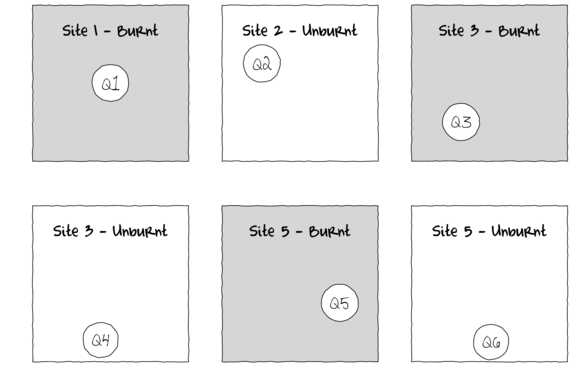
In the depiction of a single factor ANOVA below, a single quadrat has been randomly placed in each of the six Sites. If the conditions within each site were very heterogeneous, then the exact location of the quadrat in the site is likely to be very important.
As a result, the amount of variation within the main treatment effect (unexplained variability or noise) remains high thereby potentially masking any detectable effects (the signal) due to the measured treatments. Although this problem can be addressed by increased replication (having more sites of each treatment type), this is not always practical or possible.
For example, if we were investigating the impacts of fuel reduction burning across a highly heterogeneous landscape, our ability to replicate adequately might be limited by the number of burn sites available.
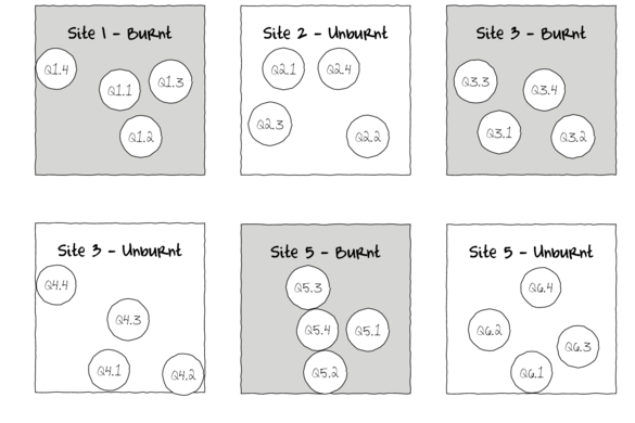
Alternatively, sub-replicates within each of the sampling units (e.g.~sites) can be collected (and averaged) so as to provided better representatives for each of the units (see the figure below) and ultimately reduce the unexplained variability of the test of treatments.
In essence, the sub-replicates are the replicates of an additional nested factor whose levels are nested within the main treatment factor. A nested factor refers to a factor whose levels are unique within each level of the factor it is nested within and each level is only represented once.
For example, the fuel reduction burn study design could consist of three burnt sites and three un-burnt (control) sites each containing four quadrats (replicates of site and sub-replicates of the burn treatment). Each site represents a unique level of a random factor (any given site cannot be both burnt and un-burnt) that is nested within the fire treatment (burned or not).
A nested design can be thought of as a hierarchical arrangement of factors (hence the alternative name hierarchical designs) whereby a treatment is progressively sub-replicated.
As an additional example, imagine an experiment designed to comparing the leaf toughness of a number of tree species. Working down the hierarchy, five individual trees were randomly selected within (nested within) each species, three branches were randomly selected within each tree, two leaves were randomly selected within each branch and the force required to shear the leaf material in half (transversely) was measured in four random locations along the leaf. Clearly any given leaf can only be from a single branch, tree and species.
Each level of sub-replication is introduced to further reduce the amount of unexplained variation and thereby increasing the power of the test for the main treatment effect. Additionally, it is possible to investigate which scale has the greatest (or least, etc) degree of variability - the level of the species, individual tree, branch, leaf, leaf region etc.
Nested factors are typically random factors, of which the levels are randomly selected to represent all possible levels (e.g.~sites). When the main treatment effect (often referred to as Factor A) is a fixed factor, such designs are referred to as a mixed model nested ANOVA, whereas when Factor A is random, the design is referred to as a Model II nested ANOVA.
Fixed nested factors are also possible. For example, specific dates (corresponding to particular times during a season) could be nested within season. When all factors are fixed, the design is referred to as a Model I mixed model.
Fully nested designs (the topic of this chapter) differ from other multi-factor designs in that all factors within (below) the main treatment factor are nested and thus interactions are un-replicated and cannot be tested. Indeed, interaction effects (interaction between Factor A and site) are assumed to be zero.
Linear models
The linear models for two and three factor nested design are:
$$y_{ijk}=\mu+\alpha_i + \beta_{j(i)} + \varepsilon_{ijk}$$
$$y_{ijkl}=\mu+\alpha_i + \beta_{j(i)} + \gamma_{k(j(i))} + \varepsilon_{ijkl}$$
where $\mu$ is the overall mean, $\alpha$ is the effect of Factor A, $\beta$ is the effect of Factor B, $\gamma$ is the effect of Factor C and $\varepsilon$ is the random unexplained or residual component.
Null hypotheses
Separate null hypotheses are associated with each of the factors, however, nested factors are typically only added to absorb some of the unexplained variability and thus, specific hypotheses tests associated with nested factors are of lesser biological importance. Hence, rather than estimate the effects of random effects, we instead estimate how much variability they contribute.
Factor A - the main treatment effect
Fixed
H$_0(A)$: $\mu_1=\mu_2=...=\mu_i=\mu$ (the population group means are all equal)
The mean of population 1 is equal to that of population 2 and so on, and thus all population means are equal to an overall mean.
If the effect of the $i^{th}$ group is the difference between the $i^{th}$ group mean and the overall mean ($\alpha_i = \mu_i - \mu$) then the H$_0$ can alternatively be written as:
H$_0(A)$: $\alpha_1 = \alpha_2 = ... = \alpha_i = 0$ (the effect of each group equals zero)
If one or more of the $\alpha_i$ are different from zero (the response mean for this treatment differs from the overall response mean), the null hypothesis is not true indicating that the treatment does affect the response variable.
Random
H$_0(A)$: $\sigma_\alpha^2=0$ (population variance equals zero)
There is no added variance due to all possible levels of A.
Factor B - the nested factor
Random (typical case)
H$_0(B)$: $\sigma_\beta^2=0$ (population variance equals zero)
There is no added variance due to all possible levels of B within the (set or all possible) levels of A.
Fixed
H$_0(B)$: $\mu_{1(1)}=\mu_{2(1)}=...=\mu_{j(i)}=\mu$ (the population group means of B (within A) are all equal)
H$_0(B)$: $\beta_{1(1)} = \beta_{2(1)}= ... = \beta_{j(i)} = 0$ (the effect of each chosen B group equals zero)
The null hypotheses associated with additional factors, are treated similarly to Factor B above.
Analysis of variance
Analysis of variance sequentially partitions the total variability in the response variable into components explained by each of the factors (starting with the factors lowest down in the hierarchy - the most deeply nested) and the components unexplained by each factor. Explained variability is calculated by subtracting the amount unexplained by the factor from the amount unexplained by a reduced model that does not contain the factor.
When the null hypothesis for a factor is true (no effect or added variability), the ratio of explained and unexplained components for that factor (F-ratio) should follow a theoretical F-distribution with an expected value less than 1. The appropriate unexplained residuals and therefore the appropriate F-ratios for each factor differ according to the different null hypotheses associated with different combinations of fixed and random factors in a nested linear model (see Table below).
| A fixed/random, B random | A fixed/random, B fixed | ||||||
|---|---|---|---|---|---|---|---|
| Factor | d.f | MS | F-ratio | Var. comp. | F-ratio | Var.comp. | |
| A | $a-1$ | $MS_A$ | $\frac{MS_A}{MS_{B^{\prime}(A)}}$ | $\frac{MS_A - MS_{B^{\prime}(A)}}{nb}$ | $\frac{MS_A}{MS_{Resid}}$ | $\frac{MS_A - MS_{Resid}}{nb}$ | |
| B$^{\prime}$(A) | $(b-1)a$ | $MS_{B^{\prime}(A)}$ | $\frac{MS_{B^{\prime}(A)}}{MS_{Resid}}$ | $\frac{MS_{B^{\prime}(A)} - MS_{Resid}}{n}$ | $\frac{MS_{B^{\prime}(A)}}{MS_{Resid}}$ | $\frac{MS_{B^{\prime}(A)} - MS_{Resid}}{n}$ | |
| Residual (=$N^{\prime}(B^{\prime}(A))$) | $(n-1)ba$ | $MS_{Resid}$ | |||||
| A fixed/random, B random | |||||||
> summary(aov(y ~ A + Error(B), data)) > library(nlme) > VarCorr(lme(y ~ A, random = 1 | B, data)) |
|||||||
| Unbalanced |
> library(nlme) > anova(lme(y ~ A, random = 1 | B, data), type = "marginal") |
||||||
| A fixed/random, B fixed | |||||||
> summary(aov(y ~ A + B, data)) |
|||||||
| Unbalanced |
> contrasts(data$B) <- contr.sum > library(car) > Anova(aov(y ~ A/B, data), type = "III") |
||||||
Variance components
As previously alluded to, it can often be useful to determine the relative contribution (to explaining the unexplained variability) of each of the factors as this provides insights into the variability at each different scales.
These contributions are known as Variance components and are estimates of the added variances due to each of the factors. For consistency with leading texts on this topic, I have included estimated variance components for various balanced nested ANOVA designs in the above table. However, variance components based on a modified version of the maximum likelihood iterative model fitting procedure (REML) is generally recommended as this accommodates both balanced and unbalanced designs.
While there are no numerical differences in the calculations of variance components for fixed and random factors, fixed factors are interpreted very differently and arguably have little biological meaning (other to infer relative contribution). For fixed factors, variance components estimate the variance between the means of the specific populations that are represented by the selected levels of the factor and therefore represent somewhat arbitrary and artificial populations. For random factors, variance components estimate the variance between means of all possible populations that could have been selected and thus represents the true population variance.
Assumptions
An F-distribution represents the relative frequencies of all the possible F-ratio's when a given null hypothesis is true and certain assumptions about the residuals (denominator in the F-ratio calculation) hold.
Consequently, it is also important that diagnostics associated with a particular hypothesis test reflect the denominator for the appropriate F-ratio. For example, when testing the null hypothesis that there is no effect of Factor A (H$_0(A): \alpha_i=0$) in a mixed nested ANOVA, the means of each level of Factor B are used as the replicates of Factor A.
As with single factor anova, hypothesis testing for nested ANOVA assumes the residuals are:
- normally distributed. Factors higher up in the hierarchy of a nested model are based on means (or means of means) of lower factors and thus the Central Limit Theory would predict that normality will usually be satisfied for the higher level factors. Nevertheless, boxplots using the appropriate scale of replication should be used to explore normality. Scale transformations are often useful.
- equally varied. Boxplots and plots of means against variance (using the appropriate scale of replication) should be used to explore the spread of values. Residual plots should reveal no patterns (see Figure~\ref{fig:correlationRegression.residualPlotDiagnostics}). Scale transformations are often useful.
- independent of one another - this requires special consideration so as to ensure that the scale at which sub-replicates are measured is still great enough to enable observations to be independent.
Pooling denominator terms
Designs that incorporate fixed and random factors (either nested or factorial), involve F-ratio calculations in which the denominators are themselves random factors other than the overall residuals. Many statisticians argue that when such denominators are themselves not statistically significant (at the 0.25 level), there are substantial power benefits from pooling together successive non-significant denominator terms. Thus an F-ratio for a particular factor might be recalculated after pooling together its original denominator with its denominators denominator and so on.
The conservative 0.25 is used instead of the usual 0.05 to reduce further the likelihood of Type II errors (falsely concluding an effect is non-significant - that might result from insufficient power).
Unbalanced nested designs
For a simple completely balanced nested ANOVA, it is possible to pool together (calculate their mean) each of the sub-replicates within each nest (=site) and then perform single factor ANOVA on those aggregates. Indeed, for a balanced design, the estimates and hypothesis for Factor A will be identical to that produced via nested ANOVA.
However, if there are an unequal number of sub-replicates within each nest, then the single factor ANOVA will be less powerful that a proper nested ANOVA.
Unbalanced designs are those designs in which sample (subsample) sizes for each level of one or more factors differ. These situations are relatively common in biological research, however such imbalance has some important implications for nested designs.
- Firstly, hypothesis tests are more robust to the assumptions of normality and equal variance when the design is balanced.
- Secondly (and arguably, more importantly), the model contrasts are not orthogonal (independent) and the sums of squares component attributed to each of the model terms cannot be calculated by simple additive partitioning of the total sums of squares.
The severity of this issue depends on which scale of the sub-sampling hierarchy the unbalance(s) occurs as well whether the unbalance occurs in the replication of a fixed or random factor. For example, whilst unequal levels of the first nesting factor (e.g. unequal number of burn vs un-burnt sites) has no effect on F-ratio construction or hypothesis testing for the top level factor (irrespective of whether either of the factors are fixed or random), unequal sub-sampling (replication) at the level of a random (but not fixed) nesting factor will impact on the ability to construct F-ratios and variance components of all terms above it in the hierarchy.
There are a number of alternative ways of dealing with unbalanced nested designs. All alternatives assume that the imbalance is not a direct result of the treatments themselves. Such outcomes are more appropriately analysed by modelling the counts of surviving observations via frequency analysis.
- Split the analysis up into separate smaller simple ANOVA's each using the means of the nesting factor to reflect the appropriate scale of replication. As the resulting sums of squares components are thereby based on an aggregated dataset the analyses then inherit the procedures and requirements of single ANOVA.
- Adopt mixed-modelling techniques (see below).
Linear mixed effects models
Although the term `mixed-effects' can be used to refer to any design that incorporates both fixed and random predictors, its use is more commonly restricted to designs in which factors are nested or grouped within other factors. Typical examples include nested, longitudinal (measurements repeated over time) data, repeated measures and blocking designs.
Furthermore, rather than basing parameter estimations on observed and expected mean squares or error strata (as outline above), mixed-effects models estimate parameters via maximum likelihood (ML) or residual maximum likelihood (REML). In so doing, mixed-effects models more appropriately handle estimation of parameters, effects and variance components of unbalanced designs (particularly for random effects).
Resulting fitted (or expected) values of each level of a factor (for example, the expected population site means) are referred to as Best Linear Unbiased Predictors (BLUP's). As an acknowledgement that most estimated site means will be more extreme than the underlying true population means they estimate (based on the principle that smaller sample sizes result in greater chances of more extreme observations and that nested sub-replicates are also likely to be highly intercorrelated), BLUP's are less spread from the overall mean than are simple site means. In addition, mixed-effects models naturally model the 'within-block' correlation structure that complicates many longitudinal designs.
Whilst the basic concepts of mixed-effects models have been around for a long time, recent computing advances and adoptions have greatly boosted the popularity of these procedures.
Linear mixed effects models are currently at the forefront of statistical development, and as such, are very much a work in progress - both in theory and in practice. Recent developments have seen a further shift away from the traditional practices associated with degrees of freedom, probability distribution and p-value calculations.
The traditional approach to inference testing is to compare the fit of an alternative (full) model to a null (reduced) model (via an F-ratio). When assumptions of normality and homogeneity of variance apply, the degrees of freedom are easily computed and the F-ratio has an exact F-distribution to which it can be compared.
However, this approach introduces two additional problematic assumptions when estimating fixed effects in a mixed effects model. Firstly, when estimating the effects of one factor, the parameter estimates associated with other factor(s) are assumed to be the true values of those parameters (not estimates). Whilst this assumption is reasonable when all factors are fixed, as random factors are selected such that they represent one possible set of levels drawn from an entire population of possible levels for the random factor, it is unlikely that the associated parameter estimates accurately reflect the true values. Consequently, there is not necessarily an appropriate F-distribution.
Furthermore, determining the appropriate degrees of freedom (nominally, the number of independent observations on which estimates are based) for models that incorporate a hierarchical structure is only possible under very specific circumstances (such as completely balanced designs).
Degrees of freedom is a somewhat arbitrary defined concept used primarily to select a theoretical probability distribution on which a statistic can be compared. Arguably, however, it is a concept that is overly simplistic for complex hierarchical designs.
Most statistical applications continue to provide the `approximate' solutions (as did earlier versions within R). However, R linear mixed effects development leaders argue strenuously that given the above shortcomings, such approximations are variably inappropriate and are thus omitted.
MCMC sampling
Markov chain Monte Carlo (MCMC) sampling methods provide a Bayesian-like alternative for inference testing. Markov chains use the mixed model parameter estimates to generate posterior probability distributions of each parameter from which Monte Carlo sampling methods draw a large set of parameter samples.
These parameter samples can then be used to calculate highest posterior density (HPD) intervals (also known as Bayesian credible intervals). Such intervals indicate the interval in which there is a specified probability (typically 95%) that the true population parameter lies. Furthermore, whilst technically against the spirit of the Bayesian philosophy, it is also possible to generate P values on which to base inferences.
Nested ANOVA in R
Scenario and Data
Imagine we has designed an experiment in which we intend to measure a response ($y$) to one of treatments (three levels; 'a1', 'a2' and 'a3'). The treatments occur at a spatial scale (over an area) that far exceeds the logistical scale of sampling units (it would take too long to sample at the scale at which the treatments were applied). The treatments occurred at the scale of hectares whereas it was only feasible to sample $y$ using 1m quadrats.
Given that the treatments were naturally occurring (such as soil type), it was not possible to have more than five sites of each treatment type, yet prior experience suggested that the sites in which you intended to sample were very uneven and patchy with respect to $y$.
In an attempt to account for this inter-site variability (and thus maximize the power of the test for the effect of treatment, you decided to employ a nested design in which 10 quadrats were randomly located within each of the five replicate sites per three treatments. As this section is mainly about the generation of artificial data (and not specifically about what to do with the data), understanding the actual details are optional and can be safely skipped. Consequently, I have folded (toggled) this section away.
- the number of treatments = 3
- the number of sites per treatment = 5
- the total number of sites = 15
- the sample size per treatment= 5
- the number of quadrats per site = 10
- the mean of the treatments = 40, 70 and 80 respectively
- the variability (standard deviation) between sites of the same treatment = 12
- the variability (standard deviation) between quadrats within sites = 5
> set.seed(1)
> nTreat <- 3
> nSites <- 15
> nSitesPerTreat <- nSites/nTreat
> nQuads <- 10
> site.sigma <- 12
> sigma <- 5
> n <- nSites * nQuads
> sites <- gl(n = nSites, k = nQuads)
> A <- gl(nTreat, nSitesPerTreat * nQuads, n, labels = c("a1", "a2", "a3"))
> a.means <- c(40, 70, 80)
> ## the site means (treatment effects) are drawn from normal distributions with means of 40, 70 and 80
> ## and standard deviations of 12
> A.effects <- rnorm(nSites, rep(a.means, each = nSitesPerTreat), site.sigma)
> # A.effects <- a.means %*% t(model.matrix(~A,
> # data.frame(A=gl(nTreat,nSitesPerTreat,nSites))))+rnorm(nSites,0,site.sigma)
> Xmat <- model.matrix(~sites - 1)
> lin.pred <- Xmat %*% c(A.effects)
> ## the quadrat observations (within sites) are drawn from normal distributions with means according to
> ## the site means and standard deviations of 5
> y <- rnorm(n, lin.pred, sigma)
> data <- data.frame(y = y, A = A, Sites = sites, Quads = 1:length(y))
> head(data)  #print out the first six rows of the data set
      y  A Sites Quads
1 32.26 a1     1     1
2 32.40 a1     1     2
3 37.20 a1     1     3
4 36.59 a1     1     4
5 35.45 a1     1     5
6 37.08 a1     1     6
> library(ggplot2)
> ggplot(data, aes(y = y, x = 1)) + geom_boxplot() + facet_grid(. ~ Sites)

> replications(y ~ A + Error(Sites), data)
 A
50
> replications(y ~ A + Sites, data)
    A Sites
   50    10
>
> data.aov <- aov(y ~ A + Error(Sites), data)
> summary(data.aov)
Error: Sites
          Df Sum Sq Mean Sq F value Pr(>F)
A          2  38547   19273    10.2 0.0026 **
Residuals 12  22615    1885
---
Signif. codes:  0 '***' 0.001 '**' 0.01 '*' 0.05 '.' 0.1 ' ' 1

Error: Within
           Df Sum Sq Mean Sq F value Pr(>F)
Residuals 135   2581    19.1
>
> library(nlme)
> data.lme <- lme(y ~ A, random = ~1 | Sites, data)
> summary(data.lme)
Linear mixed-effects model fit by REML
 Data: data
    AIC   BIC logLik
  927.7 942.7 -458.9

Random effects:
 Formula: ~1 | Sites
        (Intercept) Residual
StdDev:       13.66    4.372

Fixed effects: y ~ A
            Value Std.Error  DF t-value p-value
(Intercept) 42.28     6.139 135   6.887  0.0000
Aa2         29.85     8.682  12   3.438  0.0049
Aa3         37.02     8.682  12   4.264  0.0011
 Correlation:
    (Intr) Aa2
Aa2 -0.707
Aa3 -0.707  0.500

Standardized Within-Group Residuals:
      Min        Q1       Med        Q3       Max
-2.603787 -0.572952  0.004954  0.620915  2.765602

Number of Observations: 150
Number of Groups: 15
> VarCorr(data.lme)
Sites = pdLogChol(1)
            Variance StdDev
(Intercept) 186.55   13.658
Residual     19.12    4.372
> anova(data.lme)
            numDF denDF F-value p-value
(Intercept)     1   135   331.8  <.0001
A               2    12    10.2  0.0026
> library(multcomp)
> summary(glht(data.lme, linfct = mcp(A = "Tukey")))
	 Simultaneous Tests for General Linear Hypotheses

Multiple Comparisons of Means: Tukey Contrasts


Fit: lme.formula(fixed = y ~ A, data = data, random = ~1 | Sites)

Linear Hypotheses:
             Estimate Std. Error z value Pr(>|z|)
a2 - a1 == 0    29.85       8.68    3.44   0.0017 **
a3 - a1 == 0    37.02       8.68    4.26   <0.001 ***
a3 - a2 == 0     7.17       8.68    0.83   0.6867
---
Signif. codes:  0 '***' 0.001 '**' 0.01 '*' 0.05 '.' 0.1 ' ' 1
(Adjusted p values reported -- single-step method)
> set.seed(1)
> nTreat <- 3
> nSites <- 15
> nSitesPerTreat <- nSites/nTreat
> nQuads <- 5
> nPits <- 2
> site.sigma <- 15
> quad.sigma <- 10
> sigma <- 5
> n <- nSites * nQuads * nPits
> sites <- gl(n = nSites, n/nSites, n, lab = paste("site", 1:nSites))
> A <- gl(nTreat, n/nTreat, n, labels = c("a1", "a2", "a3"))
> a.means <- c(40, 70, 80)
>
> # A<-gl(nTreat,nSites/nTreat,nSites,labels=c('a1','a2','a3'))
> A <- gl(nTreat, 1, nTreat, labels = c("a1", "a2", "a3"))
> a.X <- model.matrix(~A, expand.grid(A))
> a.eff <- as.vector(solve(a.X, a.means))
> # a.X <- model.matrix(~A, expand.grid(A=gl(nTreat,nSites/nTreat,nSites,labels=c('a1','a2','a3'))))
> site.means <- rnorm(nSites, a.X %*% a.eff, site.sigma)
>
> SITES <- gl(nSites, 1, nSites, labels = paste("site", 1:nSites))
> sites.X <- model.matrix(~SITES - 1)
> # sites.eff <- as.vector(solve(sites.X,site.means)) quad.means <- rnorm(nSites*nQuads,sites.X %*%
> # sites.eff,quad.sigma)
> quad.means <- rnorm(nSites * nQuads, sites.X %*% site.means, quad.sigma)
>
> QUADS <- gl(nQuads, nSites, n, labels = paste("quad", 1:nQuads))
> quads.X <- model.matrix(~SITES * QUADS, expand.grid(SITES = SITES, QUADS = factor(1:nQuads)))
> quads.eff <- as.vector(solve(quads.X, quad.means))
> pit.means <- rnorm(n, quads.eff %*% t(quads.X), sigma)
>
> PITS <- gl(nPits, nSites * nQuads, n, labels = paste("pit", 1:nPits))
> data <- data.frame(Pits = PITS, Quads = QUADS, Sites = rep(SITES, 5), A = rep(A, 50), y = pit.means)
> data <- data[order(data$A, data$Sites, data$Quads), ]
> head(data)  #print out the first six rows of the data set
     Pits  Quads  Sites  A     y
1   pit 1 quad 1 site 1 a1 27.44
76  pit 2 quad 1 site 1 a1 41.18
16  pit 1 quad 2 site 1 a1 53.03
91  pit 2 quad 2 site 1 a1 38.03
31  pit 1 quad 3 site 1 a1 21.00
106 pit 2 quad 3 site 1 a1 18.29
> library(ggplot2)
> ggplot(data, aes(y = y, x = 1)) + geom_boxplot() + facet_grid(. ~ Sites * Quads)

> replications(y ~ A + Error(Sites/Quads), data)
 A
50
> replications(y ~ A + Sites + Quads, data)
    A Sites Quads
   50    10    30
>
> data.aov <- aov(y ~ A + Error(Sites/Quads), data)
> summary(data.aov)
Error: Sites
          Df Sum Sq Mean Sq F value Pr(>F)
A          2  38181   19091    7.39 0.0081 **
Residuals 12  31011    2584
---
Signif. codes:  0 '***' 0.001 '**' 0.01 '*' 0.05 '.' 0.1 ' ' 1

Error: Sites:Quads
          Df Sum Sq Mean Sq F value Pr(>F)
Residuals 60   9200     153

Error: Within
          Df Sum Sq Mean Sq F value Pr(>F)
Residuals 75   1893    25.2
>
> library(nlme)
> data.lme <- lme(y ~ A, random = ~1 | Sites/Quads/Pits, data)
> summary(data.lme)
Linear mixed-effects model fit by REML
 Data: data
   AIC  BIC logLik
  1081 1102 -533.6

Random effects:
 Formula: ~1 | Sites
        (Intercept)
StdDev:       15.59

 Formula: ~1 | Quads %in% Sites
        (Intercept)
StdDev:       8.003

 Formula: ~1 | Pits %in% Quads %in% Sites
        (Intercept) Residual
StdDev:       4.258    2.665

Fixed effects: y ~ A
            Value Std.Error DF t-value p-value
(Intercept) 43.49     7.189 75   6.049  0.0000
Aa2         30.51    10.167 12   3.001  0.0110
Aa3         36.40    10.167 12   3.580  0.0038
 Correlation:
    (Intr) Aa2
Aa2 -0.707
Aa3 -0.707  0.500

Standardized Within-Group Residuals:
     Min       Q1      Med       Q3      Max
-1.06110 -0.25122 -0.01323  0.22127  1.04089

Number of Observations: 150
Number of Groups:
                     Sites           Quads %in% Sites Pits %in% Quads %in% Sites
                        15                         75                        150
> VarCorr(data.lme)
            Variance     StdDev
Sites =     pdLogChol(1)
(Intercept) 243.091      15.591
Quads =     pdLogChol(1)
(Intercept)  64.048       8.003
Pits =      pdLogChol(1)
(Intercept)  18.132       4.258
Residual      7.101       2.665
> anova(data.lme)
            numDF denDF F-value p-value
(Intercept)     1    75  251.28  <.0001
A               2    12    7.39  0.0081
> library(multcomp)
> summary(glht(data.lme, linfct = mcp(A = "Tukey")))
	 Simultaneous Tests for General Linear Hypotheses

Multiple Comparisons of Means: Tukey Contrasts


Fit: lme.formula(fixed = y ~ A, data = data, random = ~1 | Sites/Quads/Pits)

Linear Hypotheses:
             Estimate Std. Error z value Pr(>|z|)
a2 - a1 == 0    30.51      10.17    3.00  0.00747 **
a3 - a1 == 0    36.40      10.17    3.58  0.00098 ***
a3 - a2 == 0     5.89      10.17    0.58  0.83126
---
Signif. codes:  0 '***' 0.001 '**' 0.01 '*' 0.05 '.' 0.1 ' ' 1
(Adjusted p values reported -- single-step method)
>
>
> library(glmmBUGS)
> a <- glmmBUGS(y ~ A, effects = c("Sites", "Quads"), data = data, family = "gaussian")