Tutorial 9.8a - Randomized Complete Block ANOVA
14 Jan 2014
If you are completely ontop of the conceptual issues pertaining to Nested ANOVA, and just need to use this tutorial in order to learn about Nested ANOVA in R, you are invited to skip down to the section on Nested ANOVA in R.
Overview
When single sampling units are selected amongst highly heterogeneous conditions, it is unlikely that these single units will adequately represent the populations and repeated sampling is likely to yield very different outcomes.
Tutorial 9.7a (Nested ANOVA), introduced the concept of employing sub-replicates that are nested within the main treatment levels as a means of absorbing some of the unexplained variability that would otherwise arise from designs in which sampling units are selected from amongst highly heterogeneous conditions. Such (nested) designs are useful in circumstances where the levels of the main treatment (such as burnt and un-burnt sites) occur at a much larger temporal or spatial scale than the experimental/sampling units (e.g. vegetation monitoring quadrats).
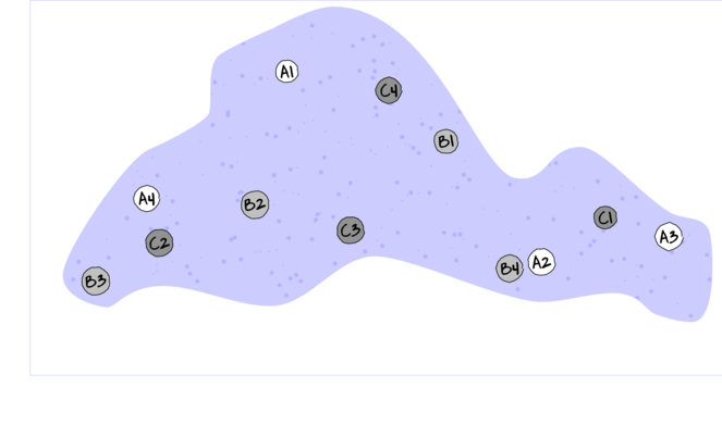
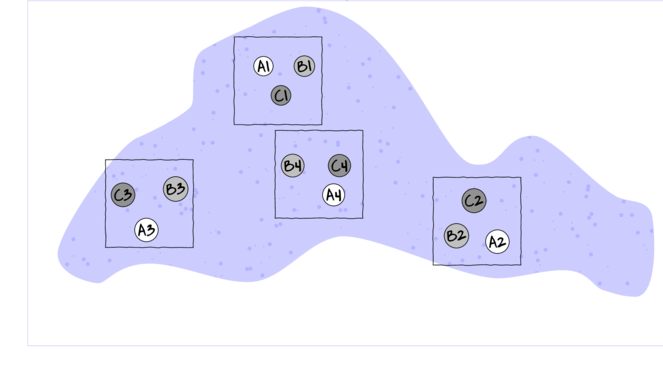
For circumstances in which the main treatments can be applied (or naturally occur) at the same scale as the sampling units (such as whether a stream rock is enclosed by a fish proof fence or not), an alternative design is available. In this design (randomized complete block design), each of the levels of the main treatment factor are grouped (blocked) together (in space and/or time) and therefore, whilst the conditions between the groups (referred to as `blocks') might vary substantially, the conditions under which each of the levels of the treatment are tested within any given block are far more homogeneous (see Figure below).
If any differences between blocks (due to the heterogeneity) can account for some of the total variability between the sampling units (thereby reducing the amount of variability that the main treatment(s) failed to explain), then the main test of treatment effects will be more powerful/sensitive.
As an simple example of a randomized complete block (RCB) design, consider an investigation into the roles of different organism scales (microbial, macro invertebrate and vertebrate) on the breakdown of leaf debris packs within streams. An experiment could consist of four treatment levels - leaf packs protected by fish-proof mesh, leaf packs protected by fine macro invertebrate exclusion mesh, leaf packs protected by dissolving antibacterial tablets, and leaf packs relatively unprotected as controls.
As an acknowledgement that there are many other unmeasured factors that could influence leaf pack breakdown (such as flow velocity, light levels, etc) and that these are likely to vary substantially throughout a stream, the treatments are to be arranged into groups or 'blocks' (each containing a single control, microbial, macro invertebrate and fish protected leaf pack). Blocks of treatment sets are then secured in locations haphazardly selected throughout a particular reach of stream. Importantly, the arrangement of treatments in each block must be randomized to prevent the introduction of some systematic bias - such as light angle, current direction etc.
Blocking does however come at a cost. The blocks absorb both unexplained variability as well as degrees of freedom from the residuals. Consequently, if the amount of the total unexplained variation that is absorbed by the blocks is not sufficiently large enough to offset the reduction in degrees of freedom (which may result from either less than expected heterogeneity, or due to the scale at which the blocks are established being inappropriate to explain much of the variation), for a given number of sampling units (leaf packs), the tests of main treatment effects will suffer power reductions.
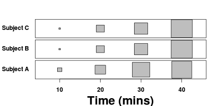
Treatments can also be applied sequentially or repeatedly at the scale of the entire block, such that at any single time, only a single treatment level is being applied (see the lower two sub-figures above). Such designs are called repeated measures. A repeated measures ANOVA is to an single factor ANOVA as a paired t-test is to a independent samples t-test.
One example of a repeated measures analysis might be an investigation into the effects of a five different diet drugs (four doses and a placebo) on the food intake of lab rats. Each of the rats (`subjects') is subject to each of the four drugs (within subject effects) which are administered in a random order.
In another example, temporal recovery responses of sharks to bi-catch entanglement stresses might be simulated by analyzing blood samples collected from captive sharks (subjects) every half hour for three hours following a stress inducing restraint. This repeated measures design allows the anticipated variability in stress tolerances between individual sharks to be accounted for in the analysis (so as to permit more powerful test of the main treatments). Furthermore, by performing repeated measures on the same subjects, repeated measures designs reduce the number of subjects required for the investigation.
Essentially, this is a randomized complete block design except that the within subject (block) effect (e.g. time since stress exposure) cannot be randomized (the consequences of which are discussed in section on Sphericity).
To suppress contamination effects resulting from the proximity of treatment sampling units within a block, units should be adequately spaced in time and space. For example, the leaf packs should not be so close to one another that the control packs are effected by the antibacterial tablets and there should be sufficient recovery time between subsequent drug administrations.
In addition, the order or arrangement of treatments within the blocks must be randomized so as to prevent both confounding as well as computational complications (Sphericity). Whilst this is relatively straight forward for the classic randomized complete block design (such as the leaf packs in streams), it is logically not possible for repeated measures designs.
Blocking factors are typically random factors (see section~\ref{chpt:ANOVA.fixedVsRandomFactor}) that represent all the possible blocks that could be selected. As such, no individual block can truly be replicated. Randomized complete block and repeated measures designs can therefore also be thought of as un-replicated factorial designs in which there are two or more factors but that the interactions between the blocks and all the within block factors are not replicated.
Linear models
The linear models for two and three factor nested design are:
$$
\begin{align}
y_{ij}&=\mu+\beta_{i}+\alpha_j + \varepsilon_{ij} &\hspace{2em} \varepsilon_{ij} &\sim\mathcal{N}(0,\sigma^2), \hspace{1em}\sum{}{\beta=0}\\
y_{ijk}&=\mu+\beta_{i} + \alpha_j + \gamma_{k} + \beta\alpha_{ij} + \beta\gamma_{ik} + \alpha\gamma_{jk} + \gamma\alpha\beta_{ijk} + \varepsilon_{ijk} \hspace{2em} (Model 1)\\
y_{ijk}&=\mu+\beta_{i} + \alpha_j + \gamma_{k} + \alpha\gamma_{jk} + \varepsilon_{ijk} (Model 2)
\end{align}
$$
where $\mu$ is the overall mean, $\beta$ is the effect of the Blocking
Factor B, $\alpha$ and $\gamma$ are the effects of withing block Factor A
and Factor C respectively and $\varepsilon$ is the random unexplained or
residual component.
Tests for the effects of blocks as well as effects within blocks assume that there are no interactions between blocks and the within block effects. That is, it is assumed that any effects are of similar nature within each of the blocks. Whilst this assumption may well hold for experiments that are able to consciously set the scale over which the blocking units are arranged, when designs utilize arbitrary or naturally occurring blocking units, the magnitude and even polarity of the main effects are likely to vary substantially between the blocks.
The preferred (non-additive or `Model 1') approach to un-replicated factorial analysis of some bio-statisticians is to include the block by within subject effect interactions (e.g. $\beta\alpha$). Whilst these interaction effects cannot be formally tested, they can be used as the denominators in F-ratio calculations of their respective main effects tests (see the tables that follow).
Proponents argue that since these blocking interactions cannot be formally tested, there is no sound inferential basis for using these error terms separately. Alternatively, models can be fitted additively (`Model 2') whereby all the block by within subject effect interactions are pooled into a single residual term ($\varepsilon$). Although the latter approach is simpler, each of the within subject effects tests do assume that there are no interactions involving the blocks and that perhaps even more restrictively, that sphericity (see section Sphericity) holds across the entire design.
Null hypotheses
Separate null hypotheses are associated with each of the factors, however, blocking factors are typically only added to absorb some of the unexplained variability and therefore specific hypothesis tests associated with blocking factors are of lesser biological importance.
Factor A - the main within block treatment effect
Fixed (typical case)
H$_0(A)$: $\mu_1=\mu_2=...=\mu_i=\mu$ (the population group means of A (pooling B) are all equal)
The mean of population 1 (pooling blocks) is equal to that of population 2 and so on, and thus all population means are equal to an overall mean.
No effect of A within each block (Model 2) or over and above the effect of blocks.
If the effect of the $i^{th}$ group is the difference between the $i^{th}$ group mean and the overall mean ($\alpha_i = \mu_i - \mu$) then the H$_0$ can alternatively be written as:
H$_0(A)$: $\alpha_1 = \alpha_2 = ... = \alpha_i = 0$ (the effect of each group equals zero)
If one or more of the $\alpha_i$ are different from zero (the response mean for this treatment differs from the overall response mean), the null hypothesis is not true indicating that the treatment does affect the response variable.
Random
H$_0(A)$: $\sigma_\alpha^2=0$ (population variance equals zero)
There is no added variance due to all possible levels of A (pooling B).
Factor B - the blocking factor
Random (typical case)
H$_0(B)$: $\sigma_\beta^2=0$ (population variance equals zero)
There is no added variance due to all possible levels of B.
Fixed
H$_0(B)$: $\mu_{1}=\mu_{2}=...=\mu_{i}=\mu$ (the population group means of B are all equal)
H$_0(B)$: $\beta_{1} = \beta_{2}= ... = \beta_{i} = 0$ (the effect of each chosen B group equals zero)
The null hypotheses associated with additional within block factors, are treated similarly to Factor A above.
Analysis of Variance
Partitioning of the total variance sequentially into explained and unexplained components and F-ratio calculations predominantly follows the rules established in tutorials on Nested ANOVA and Factorial ANOVA. Randomized block and repeated measures designs can essentially be analysed as Model III ANOVAs. The appropriate unexplained residuals and therefore the appropriate F-ratios for each factor differ according to the different null hypotheses associated with different combinations of fixed and random factors and what analysis approach (Model 1 or 2) is adopted for the randomized block linear model (see the following tables).
In additively (Model 2) fitted models (in which block interactions are assumed not to exist and are thus pooled into a single residual term), hypothesis tests of the effect of B (blocking factor) are possible. However, since blocking designs are usually employed out of expectation for substantial variability between blocks, such tests are rarely of much biological interest.
| F-ratio | ||||||
|---|---|---|---|---|---|---|
| Factor | d.f | MS | Model 1 (non-additive) | Model 2 (additive) | ||
| B$^\prime$ (block) | $b-1$ | $MS_{B^\prime}$ | $\large\frac{MS_{B^\prime}}{MS_{Resid}}$ | $\large\frac{MS_{B^\prime}}{MS_{Resid}}$ | ||
| A | $a-1$ | $MS_A$ | $\large\frac{MS_A}{MS_{Resid}}$ | $\large\frac{MS_A}{MS_{Resid}}$ | ||
| Residual (=B$^\prime$A)) | $(b-1)(a-1)$ | $MS_{Resid}$ | ||||
| R syntax | ||||||
| Balanced |
> summary(aov(y ~ A + Error(B), data)) |
|||||
| Balanced or unbalanced |
> library(nlme) > summary(lme(y ~ A, random = ~1 | B, data)) > anova(lme(y ~ A, random = ~1 | B, data)) > # OR > library(lme4) > summary(lmer(y ~ (1 | B) + A, data)) |
|||||
| Variance components |
> library(nlme) > summary(lme(y ~ 1, random = ~1 | B/A, data)) > # OR > library(lme4) > summary(lmer(y ~ (1 | B) + (1 | A), data)) |
|||||
| F-ratio | ||||||||
|---|---|---|---|---|---|---|---|---|
| A&C fixed, B random | A fixed, B&C random | A,B&C random | ||||||
| Factor | d.f. | Model 1 | Model 2 | Model 1 | Model 2 | Model 1 | Model 2 | |
| 1 | B | $b-1$ | $1/7$ | $1/7$ | $1/6$ | $1/7$ | $1/(5+6-7)$ | $1/7$ |
| 2 | A | $a-1$ | $2/5$ | $2/7$ | $2/(4+5-7)$ | $2/4$ | $2/(4+5-7)$ | $1/4$ |
| 3 | C | $c-1$ | $3/6$ | $3/7$ | $3/6$ | $3/7$ | $3/(4+6-7)$ | $3/4$ |
| 4 | A$\times$C | $(a-1)(c-1)$ | $4/7$ | $4/7$ | $4/7$ | $4/7$ | $4/7$ | $4/7$ |
| 5 | B${^\prime}\times$A | $(b-1)(a-1)$ | No test | No test | $5/7$ | |||
| 6 | B${^\prime}\times$C | $(b-1)(c-1)$ | No test | No test | $6/7$ | |||
| 7 | Residuals (=B$^{\prime}\times$A$\times$C) | $(b-1)(a-1)(c-1)$ | ||||||
| B random, A&C fixed | ||||||||
| Model 1 |
> summary(aov(y ~ Error(B/(A * C)) + A * C, data)) |
|||||||
| Model 2 |
> summary(aov(y ~ Error(B) + A * C, data)) > # or > library(nlme) > summary(lme(y ~ A * C, random = ~1 | B, data)) |
|||||||
| Unbalanced |
> anova(lme(DV ~ A * C, random = ~1 | B), type = "marginal") > anova(lme(DV ~ A * C, random = ~1 | B, correlation = corAR1(form = ~1 | + B)), type = "marginal") |
|||||||
| Other models | ||||||||
> library(lmer) > summary(lmer(DV ~ (~1 | A * C) + (1 | B)), data) #for example > # or > summary(lm(y ~ A * B * C, data)) # and make manual F-ratio etc adjustments |
||||||||
| Variance components |
> library(nlme) > summary(lme(y ~ 1, random = ~1 | B/(A * C), data)) |
|||||||
Assumptions
As with other ANOVA designs, the reliability of hypothesis tests is dependent on the residuals being:
- normally distributed. Boxplots using the appropriate scale of replication (reflecting the appropriate residuals/F-ratio denominator (see Tables above) should be used to explore normality. Scale transformations are often useful.
- equally varied. Boxplots and plots of means against variance (using the appropriate scale of replication) should be used to explore the spread of values. Residual plots should reveal no patterns. Scale transformations are often useful.
- independent of one another. Although the observations within a block may not strictly be independent, provided the treatments are applied or ordered randomly within each block or subject, within block proximity effects on the residuals should be random across all blocks and thus the residuals should still be independent of one another. Nevertheless, it is important that experimental units within blocks are adequately spaced in space and time so as to suppress contamination or carryover effects.
Sphericity
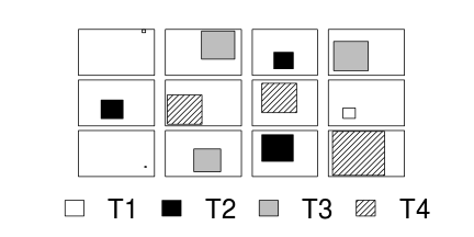
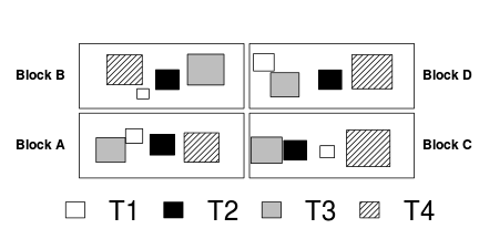
Un-replicated factorial designs extend the usual equal variance (no relationship between mean and variance) assumption to further assume that the differences between each pair of within block treatments are equally varied across the blocks (see the following figure). To meet this assumption a matrix of variances (between pairs of observations within treatments) and covariances (between treatment pairs within each block) must display a pattern known as sphericity. Strickly, the variance-covariance matrix must display a very specific pattern of sphericity in which both variances and covariances are equal (compound symmetry), however an F-ratio will still reliably follow an F distribution provided basic sphericity holds.
| Single factor ANOVA | |||||||||||||||||||||||||||
|---|---|---|---|---|---|---|---|---|---|---|---|---|---|---|---|---|---|---|---|---|---|---|---|---|---|---|---|
|
Variance-covariance structure
|
||||||||||||||||||||||||||
| Randomized Complete Block | |||||||||||||||||||||||||||
|
Variance-covariance structure
|
||||||||||||||||||||||||||
| Repeated Measures Design | |||||||||||||||||||||||||||
|
Variance-covariance structure
|
||||||||||||||||||||||||||
Typically, un-replicated factorial designs in which the treatment levels have been randomly arranged (temporally and spatially) within each block (randomized complete block) should meet this sphericity assumption. Conversely, repeated measures designs that incorporate factors whose levels cannot be randomized within each block (such as distances from a source or time), are likely to violate this assumption. In such designs, the differences between treatments that are arranged closer together (in either space or time) are likely to be less variable (greater paired covariances) than the differences between treatments that are further apart.
Hypothesis tests are not very robust to substantial deviations from sphericity and consequently tend to have inflated type I errors. There are three broad techniques for compensating or tackling the issues of sphericity:
- reducing the degrees of freedom for F tests according to the degree of departure from sphericity (measured by epsilon ($\epsilon$)). The two main estimates of epsilon are Greenhouse-Geisser and Huynh-Feldt, the former of which is preferred (as it provides more liberal protection) unless its value is less than 0.5.
- perform a multivariate ANOVA (MANOVA). Although the sphericity assumption does not apply to such procedures, MANOVA's essentially test null hypotheses about the differences between multiple treatment pairs (and thus test whether an array of population means equals zero), and therefore assume multivariate normality - a difficult assumption to explore.
- fit a linear mixed effects (lme) model and incorporate a particular correlation structure into the modelling. The approximate form of the correlation structure can be specified up-front when fitting linear mixed effects models (via lme) and thus correlated data are more appropriately handled. A selection of variance-covariance structures appropriate for biological data are listed in Table~\ref{tab:randomizedBlockAnova-correlationStructures}. It is generally recommended that linear mixed effects models be fitted with a range of covariance structures. The "best" covariance structure is that the results in a better fit (as measured by either AIC, BIC or ANOVA) than a model fitted with a compound symmetry structure.
Block by treatment interactions
The presence of block by treatment interactions have important implications for models that incorporate a single within block factor as well as additive models involving two or more within block factors. In both cases, the blocking interactions and overall random errors are pooled into a residual term that is used as the denominator in F-ratio calculations (see the tables above).
Consequently, block by treatment interactions increase the denominator ($MS_{Resid}$) resulting in lower F-ratios (lower power). Moreover, the presence of strong blocking interactions would imply that any effects of the main factor are not consistent. Drawing conclusions from such an analysis (particularly in light of non-significant main effects) is difficult. Unless we assume that there are no block by within block interactions, non-significant within block effects could be due to either an absence of a treatment effect, or as a result of opposing effects within different blocks. As these block by within block interactions are unreplicated, they can neither be formally tested nor is it possible to perform main effects tests to diagnose non-significant within block effects.
Block by treatment interactions can be diagnosed by examining;
- interaction (cell means) plot. The mean ($n=1$) response for each level of the main factor is plotted against the block number. Parallel lines infer no block by treatment interaction.
- residual plot. A curvilinear pattern in which the residual values switch from positive to negative and back again (or visa versa) over the range of predicted values implies that the scale (magnitude but not polarity) of the main treatment effects differs substantially across the range of blocks. Scale transformations can be useful in removing such interactions.
- Tukey's test for non-additivity evaluated at $\alpha=0.10$ or even $\alpha=0.25$. This (curvilinear test) formally tests for the presence of a quadratic trend in the relationship between residuals and predicted values. As such, it too is only appropriate for simple interactions of scale.
ANOVA in R
Simple RCB
Scenario and Data
Imagine we has designed an experiment in which we intend to measure a response ($y$) to one of treatments (three levels; 'a1', 'a2' and 'a3'). Unfortunately, the system that we intend to sample is spatially heterogeneous and thus will add a great deal of noise to the data that will make it difficult to detect a signal (impact of treatment).
Thus in an attempt to constrain this variability you decide to apply a design (RCB) in which each of the treatments within each of 35 blocks dispersed randomly throughout the landscape. As this section is mainly about the generation of artificial data (and not specifically about what to do with the data), understanding the actual details are optional and can be safely skipped. Consequently, I have folded (toggled) this section away.
- the number of treatments = 3
- the number of blocks containing treatments = 35
- the mean of the treatments = 40, 70 and 80 respectively
- the variability (standard deviation) between blocks of the same treatment = 12
- the variability (standard deviation) between treatments withing blocks = 5
> library(plyr)
> set.seed(1)
> nTreat <- 3
> nBlock <- 35
> sigma <- 5
> sigma.block <- 12
> n <- nBlock * nTreat
> Block <- gl(nBlock, k = 1)
> A <- gl(nTreat, k = 1)
> dt <- expand.grid(A = A, Block = Block)
> # Xmat <- model.matrix(~Block + A + Block:A, data=dt)
> Xmat <- model.matrix(~-1 + Block + A, data = dt)
> block.effects <- rnorm(n = nBlock, mean = 40, sd = sigma.block)
> A.effects <- c(30, 40)
> all.effects <- c(block.effects, A.effects)
> lin.pred <- Xmat %*% all.effects
>
> # OR
> Xmat <- cbind(model.matrix(~-1 + Block, data = dt), model.matrix(~-1 + A, data = dt))
> ## Sum to zero block effects
> block.effects <- rnorm(n = nBlock, mean = 0, sd = sigma.block)
> A.effects <- c(40, 70, 80)
> all.effects <- c(block.effects, A.effects)
> lin.pred <- Xmat %*% all.effects
>
>
>
> ## the quadrat observations (within sites) are drawn from normal distributions with means according to
> ## the site means and standard deviations of 5
> y <- rnorm(n, lin.pred, sigma)
> data <- data.frame(y = y, expand.grid(A = A, Block = Block))
> head(data)  #print out the first six rows of the data set
      y A Block
1 37.40 1     1
2 61.47 2     1
3 78.07 3     1
4 30.60 1     2
5 59.00 2     2
6 76.73 3     2
Exploratory data analysis
Normality and Homogeneity of variance
> boxplot(y ~ A, data)

Conclusions:
- there is no evidence that the response variable is consistently non-normal across all populations - each boxplot is approximately symmetrical
- there is no evidence that variance (as estimated by the height of the boxplots) differs between the five populations. . More importantly, there is no evidence of a relationship between mean and variance - the height of boxplots does not increase with increasing position along the y-axis. Hence it there is no evidence of non-homogeneity
- transform the scale of the response variables (to address normality etc). Note transformations should be applied to the entire response variable (not just those populations that are skewed).
Block by within-Block interaction
> library(car)
> with(data, interaction.plot(A, Block, y))

> library(car)
> residualPlots(lm(y ~ Block + A, data))

           Test stat Pr(>|t|)
Block             NA       NA
A                 NA       NA
Tukey test    -0.885    0.376
> # the Tukey's non-additivity test by itself can be obtained via an internal function within the car
> # package
> car:::tukeyNonaddTest(lm(y ~ Block + A, data))
   Test  Pvalue
-0.8854  0.3759
> # alternatively, there is also a Tukey's non-additivity test within the asbio package
> library(asbio)
> with(data, tukey.add.test(y, A, Block))
Tukey's one df test for additivity
F = 0.784   Denom df = 67    p-value = 0.3791
Conclusions:
- there is no visual or inferential evidence of any major interactions between Block and the within-Block effect (A). Any trends appear to be reasonably consistent between Blocks.
Sphericity
Since the levels of A were randomly assigned within each Block, we have no reason to expect that the variance-covariance will deviate substantially from sphericity. Nevertheless, we can calculate the epsilon sphericity values to confirm this. Recall that the closer the epsilon value is to 1, the greater the degree of sphericity compliance.
> library(biology)
> epsi.GG.HF(aov(y ~ Error(Block) + A, data = data))
$GG.eps
[1] 0.9135

$HF.eps
[1] 0.9626

$sigma
[1] 20.91
Conclusions:
- Both the Greenhouse-Geisser and Huynh-Feldt epsilons are reasonably close to one (they are both greater than 0.8), hence there is no evidence of correlation dependency structures.
Alternatively (and preferentially), we can explore whether there is an auto-correlation patterns in the residuals.
> library(nlme)
> data.lme <- lme(y ~ A, random = ~1 | Block, data = data)
> acf(resid(data.lme))

Conclusions:
- The autocorrelation factor (ACF) at a range of lags up to 20, indicate that there is not a strong pattern of a contagious structure running through the residuals. Note the ACF of lag 0 will always be 1 - the correlation of residuals with themselves must be 100%.
Model fitting or statistical analysis
In R, simple RCB ANOVA models are fit either the traditional way using the aov() function along with the Error() parameter to specify the heirarchical structure, or via one of the mixed effects models (e.g. lme or lmer). Of the mixed effects modelling tools, I still prefer the older lme as it provides a way to incorporate different variance-covariance structures.
- Traditional hierarchical ANOVA
> data.aov <- aov(y ~ Error(Block) + A, data)
- Linear mixed effects model
> library(nlme)
> # Assuming sphericity
> data.lme <- lme(y ~ A, random = ~1 | Block, data = data)
Model evaluation
Prior to exploring the model parameters, it is prudent to confirm that the model did indeed fit the assumptions and was an appropriate fit to the data.
Residuals
Not only do the residuals provide insights into the validity of the model with respect to linearity and homogeneity of variance, they provide important insights into the validity of the model with respect the variance-covariance structure in general. It is also a good idea to plot the residuals against each of the predictors to ensure that there are no obvious trends or differences in spread between the different treatments etc.
May also advocate plotting residuals against other predictors that do not appear in the model as a way to either identify latent dependency structures or else other useful covariates.
As Pearson residuals don't reflect variance-covariance structures included whilst modelling, it is best to view residual plots based on standardized residuals.
- Traditional hierarchical ANOVA
> par(mfrow = c(2, 2))
> plot(lm(data.aov), which = 1:4)

> residualPlots(lm(data.aov))

           Test stat Pr(>|t|)
A                 NA       NA
Block             NA       NA
Tukey test    -0.885    0.376
- Linear mixed effects model
> plot(data.lme)

> plot(resid(data.lme) ~ data$A)

Conclusions:
- There are no obvious patterns or issues with the residuals.
Extractor functions
There are a number of extractor functions (functions that extract or derive specific information from a model) available including:| Extractor | Description |
|---|---|
| residuals() | Extracts the residuals from the model |
| fitted() | Extracts the predicted (expected) response values (on the link scale) at the observed levels of the linear predictor |
| predict() | Extracts the predicted (expected) response values (on either the link, response or terms (linear predictor) scale) |
| coef() | Extracts the model coefficients |
| confint() | Calculate confidence intervals for the model coefficients |
| summary() | Summarizes the important output and characteristics of the model |
| anova() | Computes an analysis of variance (variance partitioning) from the model |
| plot() | Generates a series of diagnostic plots from the model |
| effect() | effects package - estimates the marginal (partial) effects of a factor (useful for plotting) |
| avPlot() | car package - generates partial regression plots |
Exploring the model parameters, test hypotheses
If there was any evidence that the assumptions had been violated, then we would need to reconsider the model and start the process again. In this case, there is no evidence that the test will be unreliable so we can proceed to explore the test statistics.
- Traditional hierarchical ANOVA
> summary(data.aov)
Error: Block
          Df Sum Sq Mean Sq F value Pr(>F)
Residuals 34  14233     419

Error: Within
          Df Sum Sq Mean Sq F value Pr(>F)
A          2  29855   14927     714 <2e-16 ***
Residuals 68   1422      21
---
Signif. codes:  0 '***' 0.001 '**' 0.01 '*' 0.05 '.' 0.1 ' ' 1
Conclusions:
- The output is split up into strata that reflect the supposed residuals (error) appropriate for
each hypothesis test.
- the first strata shows the between Block effects (of which there are none)
- the second shows the within Block effects (A) which is tested against the overall residuals (the Block:A interaction)
- There is a significant effect of $A$ on $y$
- The output is split up into strata that reflect the supposed residuals (error) appropriate for
each hypothesis test.
- Linear mixed effects model
> summary(data.lme)
Linear mixed-effects model fit by REML
 Data: data
    AIC   BIC logLik
  722.1 735.2 -356.1

Random effects:
 Formula: ~1 | Block
        (Intercept) Residual
StdDev:       11.51    4.572

Fixed effects: y ~ A
            Value Std.Error DF t-value p-value
(Intercept) 43.03     2.094 68   20.55       0
A2          28.45     1.093 68   26.03       0
A3          40.16     1.093 68   36.74       0
 Correlation:
   (Intr) A2
A2 -0.261
A3 -0.261  0.500

Standardized Within-Group Residuals:
     Min       Q1      Med       Q3      Max
-1.78748 -0.57868 -0.07108  0.49991  2.33728

Number of Observations: 105
Number of Groups: 35
The output comprises:
- various information criterion (for model comparison)
- the random effects variance components
- the estimated standard deviation between Blocks is
11.514 - the estimated standard deviation within treatments is
4.572 - Blocks represent
71.5778% of the variability (based on SD).
- the estimated standard deviation between Blocks is
- the fixed effects
- The effects parameter estimates along with their hypothesis tests
- $y$ is significantly higher with Treatment $A2$ or $A3$ than $A1$
Conclusions: there is a significant effect of Treatment on $y$.> anova(data.lme)
            numDF denDF F-value p-value
(Intercept)     1    68    1089  <.0001
A               2    68     714  <.0001
Planned comparisons and pairwise post-hoc tests
As with non-heirarchical models, we can incorporate alternative contrasts for the fixed effects (other than the default treatment contrasts). The random factors must be sum-to-zero contrasts in order to ensure that the model is identifiable (possible to estimate true values of the parameters).
Likewise, post-hoc tests such as Tukey's tests can be performed.
> library(multcomp)
> summary(glht(data.lme, linfct = mcp(A = "Tukey")))
	 Simultaneous Tests for General Linear Hypotheses

Multiple Comparisons of Means: Tukey Contrasts


Fit: lme.formula(fixed = y ~ A, data = data, random = ~1 | Block)

Linear Hypotheses:
           Estimate Std. Error z value Pr(>|z|)
2 - 1 == 0    28.45       1.09    26.0   <2e-16 ***
3 - 1 == 0    40.16       1.09    36.7   <2e-16 ***
3 - 2 == 0    11.70       1.09    10.7   <2e-16 ***
---
Signif. codes:  0 '***' 0.001 '**' 0.01 '*' 0.05 '.' 0.1 ' ' 1
(Adjusted p values reported -- single-step method)
RCB (repeated measures) ANOVA in R - continuous within
Scenario and Data
Imagine now that we has designed an experiment to investigate the effects of a continuous predictor ($x$, for example time) on a response ($y$). Again, the system that we intend to sample is spatially heterogeneous and thus will add a great deal of noise to the data that will make it difficult to detect a signal (impact of treatment).
Thus in an attempt to constrain this variability, we again decide to apply a design (RCB) in which each of the levels of X (such as time) treatments within each of 35 blocks dispersed randomly throughout the landscape. As this section is mainly about the generation of artificial data (and not specifically about what to do with the data), understanding the actual details are optional and can be safely skipped. Consequently, I have folded (toggled) this section away.
- the number of times = 10
- the number of blocks containing treatments = 35
- mean slope (rate of change in response over time) = 60
- mean intercept (value of response at time 0 = 200
- the variability (standard deviation) between blocks of the same treatment = 12
- the variability (standard deviation) in slope = 5
> library(plyr)
> set.seed(1)
> slope <- 30
> intercept <- 200
> nBlock <- 35
> nTime <- 10
> sigma <- 50
> sigma.block <- 30
> n <- nBlock * nTime
> Block <- gl(nBlock, k = 1)
> Time <- 1:10
> rho <- 0.8
> dt <- expand.grid(Time = Time, Block = Block)
> Xmat <- model.matrix(~-1 + Block + Time, data = dt)
> block.effects <- rnorm(n = nBlock, mean = intercept, sd = sigma.block)
> # A.effects <- c(30,40)
> all.effects <- c(block.effects, slope)
> lin.pred <- Xmat %*% all.effects
>
> # OR
> Xmat <- cbind(model.matrix(~-1 + Block, data = dt), model.matrix(~Time, data = dt))
> ## Sum to zero block effects block.effects <- rnorm(n = nBlock, mean = 0, sd = sigma.block) A.effects
> ## <- c(40,70,80) all.effects <- c(block.effects,intercept,slope) lin.pred <- Xmat %*% all.effects
>
> ## the quadrat observations (within sites) are drawn from normal distributions with means according to
> ## the site means and standard deviations of 5
> eps <- NULL
> eps[1] <- 0
> for (j in 2:n) {
+     eps[j] <- rho * eps[j - 1]  #residuals
+ }
> y <- rnorm(n, lin.pred, sigma) + eps
>
> # OR
> eps <- NULL
> # first value cant be autocorrelated
> eps[1] <- rnorm(1, 0, sigma)
> for (j in 2:n) {
+     eps[j] <- rho * eps[j - 1] + rnorm(1, mean = 0, sd = sigma)  #residuals
+ }
> y <- lin.pred + eps
> data <- data.frame(y = y, dt)
> head(data)  #print out the first six rows of the data set
      y Time Block
1 208.4    1     1
2 132.5    2     1
3 201.5    3     1
4 150.2    4     1
5 169.8    5     1
6 298.3    6     1
> library(ggplot2)
> ggplot(data, aes(y = y, x = Time)) + geom_smooth(method = "lm") + geom_point() + facet_wrap(~Block)

Exploratory data analysis
Normality and Homogeneity of variance
> boxplot(y ~ Time, data)

Conclusions:
- there is no evidence that the response variable is consistently non-normal across all populations - each boxplot is approximately symmetrical
- there is no evidence that variance (as estimated by the height of the boxplots) differs between the five populations. . More importantly, there is no evidence of a relationship between mean and variance - the height of boxplots does not increase with increasing position along the y-axis. Hence it there is no evidence of non-homogeneity
- transform the scale of the response variables (to address normality etc). Note transformations should be applied to the entire response variable (not just those populations that are skewed).
Block by within-Block interaction
> library(car)
> with(data, interaction.plot(Time, Block, y))

> library(car)
> residualPlots(lm(y ~ Block + Time, data))

           Test stat Pr(>|t|)
Block             NA       NA
Time           0.485    0.628
Tukey test    -0.663    0.507
> # the Tukey's non-additivity test by itself can be obtained via an internal function within the car
> # package
> car:::tukeyNonaddTest(lm(y ~ Block + Time, data))
   Test  Pvalue
-0.6629  0.5074
> # alternatively, there is also a Tukey's non-additivity test within the asbio package
> library(asbio)
> with(data, tukey.add.test(y, Time, Block))
Tukey's one df test for additivity
F = 1.2438   Denom df = 305    p-value = 0.2656
Conclusions:
- there is no visual or inferential evidence of any major interactions between Block and the within-Block effect (Time). Any trends appear to be reasonably consistent between Blocks.
Sphericity
Since the levels of Time cannot be randomly assigned, it is likely that sphericity is not met.
> library(biology)
> epsi.GG.HF(aov(y ~ Error(Block) + Time, data = data))
$GG.eps
[1] 0.3844

$HF.eps
[1] 0.4333

$sigma
[1] 4010
Conclusions:
- Both the Greenhouse-Geisser and Huynh-Feldt epsilons are very low. In fact, since the Greenhouse-Geisser epsilon is lower than 0.5, we will base any corrections on the Huynh-Feldt measure. Essentially, when using traditional ANOVA modelling, we would multiply the degrees of freedom by the epsilon value in order to lower the sensitivity of the tests. This is somewhat of a hack that attempts to compensate for inflated power by adjusting proportional to the approximate degree of severity (deviation from sphericity).
Alternatively (and preferentially), we can explore whether there is an auto-correlation patterns in the residuals. Note, as there was only ten time periods, it does not make logical sense to explore lags above 10.
> library(nlme)
> data.lme <- lme(y ~ Time, random = ~1 | Block, data = data)
> acf(resid(data.lme), lag = 10)

Conclusions:
- The autocorrelation factor (ACF) at a range of lags up to 10, indicate that there is a cyclical pattern of residual auto-correlation. We really should explore incorporating some form of correlation structure into our model.
Model fitting or statistical analysis
In R, simple RCB ANOVA models are fit either the traditional way using the aov() function along with the Error() parameter to specify the heirarchical structure, or via one of the mixed effects models (e.g. lme or lmer). Of the mixed effects modelling tools, I still prefer the older lme as it provides a way to incorporate different variance-covariance structures.
- Traditional hierarchical ANOVA
> data.aov <- aov(y ~ Error(Block) + Time, data)
> AnovaM(data.aov, RM = TRUE)
   Sphericity Epsilon Values
-------------------------------
 Greenhouse.Geisser Huynh.Feldt
             0.3844      0.4333
Anova Table (Type I tests) Response: y Error: Block Df Sum Sq Mean Sq F value Pr(>F) Residuals 34 1375910 40468 Error: Within Df Sum Sq Mean Sq F value Pr(>F) Time 1 3086554 3086554 778 <2e-16 *** Residuals 314 1245701 3967 --- Signif. codes: 0 '***' 0.001 '**' 0.01 '*' 0.05 '.' 0.1 ' ' 1 Greenhouse-Geisser corrected ANOVA table Response: y Error: Block Df Sum Sq Mean Sq F value Pr(>F) Residuals 34 1375910 40468 Error: Within Df Sum Sq Mean Sq F value Pr(>F) Time 0.384 3086554 3086554 778 <2e-16 *** Residuals 314.000 1245701 3967 --- Signif. codes: 0 '***' 0.001 '**' 0.01 '*' 0.05 '.' 0.1 ' ' 1 Huynh-Feldt corrected ANOVA table Response: y Error: Block Df Sum Sq Mean Sq F value Pr(>F) Residuals 34 1375910 40468 Error: Within Df Sum Sq Mean Sq F value Pr(>F) Time 0.433 3086554 3086554 778 <2e-16 *** Residuals 314.000 1245701 3967 --- Signif. codes: 0 '***' 0.001 '**' 0.01 '*' 0.05 '.' 0.1 ' ' 1 - Linear mixed effects model
> library(nlme)
> # Assuming sphericity
> data.lme <- lme(y ~ Time, random = ~1 | Block, data = data, method = "ML")
> data.lme.CS <- update(data.lme, correlation = corCompSymm(form = ~Time | Block))
> AIC(data.lme, data.lme.CS)
            df  AIC
data.lme     4 3981
data.lme.CS  5 3983
> data.lme.AR1 <- update(data.lme, correlation = corAR1(form = ~Time | Block))
> # since time is 1:10, the following is the same
> data.lme.AR1 <- update(data.lme, correlation = corAR1(form = ~1 | Block))
> AIC(data.lme, data.lme.AR1)
             df  AIC
data.lme      4 3981
data.lme.AR1  5 3825
> # Likelihood ratio test
> anova(data.lme, data.lme.AR1)
             Model df  AIC  BIC logLik   Test L.Ratio p-value
data.lme         1  4 3981 3996  -1986
data.lme.AR1     2  5 3825 3844  -1907 1 vs 2   157.8  <.0001
Conclusions: the linear mixed effects model that incorporates the first-order autocorrelation structure fits the data significantly better that a model that assumes compound symmetric or sphericity. We should now refit the model using REML
> library(nlme)
> data.lme.AR1 <- update(data.lme.AR1, method = "REML")
Model evaluation
Prior to exploring the model parameters, it is prudent to confirm that the model did indeed fit the assumptions and was an appropriate fit to the data.
Residuals
Not only do the residuals provide insights into the validity of the model with respect to linearity and homogeneity of variance, they provide important insights into the validity of the model with respect the variance-covariance structure in general. It is also a good idea to plot the residuals against each of the predictors to ensure that there are no obvious trends or differences in spread between the different treatments etc.
May also advocate plotting residuals against other predictors that do not appear in the model as a way to either identify latent dependency structures or else other useful covariates.
As Pearson residuals don't reflect variance-covariance structures included whilst modelling, it is best to view residual plots based on standardized residuals.
- Traditional hierarchical ANOVA
> par(mfrow = c(2, 2))
> plot(lm(data.aov), which = 1:4)

> residualPlots(lm(data.aov))

           Test stat Pr(>|t|)
Time           0.485    0.628
Block             NA       NA
Tukey test    -0.663    0.507
- Linear mixed effects model
> plot(data.lme.AR1)

> plot(resid(data.lme.AR1, type = "normalized") ~ data$Time)

> acf(resid(data.lme.AR1, type = "normalized"), lag = 10)

> # OR
> ACF(data.lme.AR1, maxlag = 10)
   lag      ACF
1    0  1.00000
2    1  0.67717
3    2  0.44011
4    3  0.23063
5    4  0.03929
6    5 -0.05311
7    6 -0.09469
8    7 -0.05436
9    8  0.02550
10   9  0.12086
Conclusions:
- There are no obvious patterns or issues with the residuals.
Exploring the model parameters, test hypotheses
If there was any evidence that the assumptions had been violated, then we would need to reconsider the model and start the process again. In this case, there is no evidence that the test will be unreliable so we can proceed to explore the test statistics.
- Traditional hierarchical ANOVA
> summary(data.aov)
Error: Block
          Df  Sum Sq Mean Sq F value Pr(>F)
Residuals 34 1375910   40468

Error: Within
           Df  Sum Sq Mean Sq F value Pr(>F)
Time        1 3086554 3086554     778 <2e-16 ***
Residuals 314 1245701    3967
---
Signif. codes:  0 '***' 0.001 '**' 0.01 '*' 0.05 '.' 0.1 ' ' 1
Conclusions:
- The output is split up into strata that reflect the supposed residuals (error) appropriate for
each hypothesis test.
- the first strata shows the between Block effects (of which there are none)
- the second shows the within Block effects (A) which is tested against the overall residuals (the Block:A interaction)
- There is a significant effect of $A$ on $y$
- The output is split up into strata that reflect the supposed residuals (error) appropriate for
each hypothesis test.
- Linear mixed effects model
> summary(data.lme.AR1)
Linear mixed-effects model fit by REML
 Data: data
   AIC  BIC logLik
  3815 3834  -1902

Random effects:
 Formula: ~1 | Block
        (Intercept) Residual
StdDev:       39.91    80.75

Correlation Structure: AR(1)
 Formula: ~1 | Block
 Parameter estimate(s):
   Phi
0.7549
Fixed effects: y ~ Time
             Value Std.Error  DF t-value p-value
(Intercept) 173.22    15.938 314   10.87       0
Time         32.13     2.041 314   15.75       0
 Correlation:
     (Intr)
Time -0.704

Standardized Within-Group Residuals:
     Min       Q1      Med       Q3      Max
-2.21889 -0.68745 -0.03738  0.59724  2.35352

Number of Observations: 350
Number of Groups: 35
> # str(summary(data.lme.AR1)) > nlme:::coef.corAR1(data.lme.AR1, unconstrained = FALSE)
Error: non-numeric argument to mathematical function
> str(as.vector(data.lme.AR1))
List of 18 $ modelStruct :List of 2 ..$ reStruct :List of 1 .. ..$ Block:Classes 'pdLogChol', 'pdSymm', 'pdMat' atomic [1:1] -0.705 .. .. .. ..- attr(*, "formula")=Class 'formula' length 2 ~1 .. .. .. .. .. ..- attr(*, ".Environment")=
The output comprises:
- various information criterion (for model comparison)
- the random effects variance components
- the estimated standard deviation between Blocks is
39.91 - the estimated standard deviation within treatments is
80.75 - Blocks represent
33.0764% of the variability (based on SD).
- the estimated standard deviation between Blocks is
- The AR1 correlation structure correlation parameter ($\phi$) is estimated to be
- the fixed effects
- The effects parameter estimates along with their hypothesis tests
- $y$ is significantly higher with Treatment $A2$ or $A3$ than $A1$