Workshop 11 - The power of Contrasts
23 April 2011
Context
- Recent statistical advice has progressively advocated the use of effect sizes and confidence intervals over the traditional p-values of hyothesis tests.
- It is argued that the size of p-values are regularly incorrectly inferred to represent the strength of an effect.
- Proponents argue that effect sizes (the magnitude of the differences between treatment levels or trajectories) and associated measures of confidence or precision of these estimates provide far more informative summaries.
- Furthermore, the resolve of these recommendations is greatly enhanced as model complexity increases (particularly with the introduction of nesting or repeated measures) and appropriate degrees of freedom on which to base p-value calculations become increasingly more tenuous.
- Consequently, there have been numerous pieces of work that oppose/criticize/impugn the use of p-values and advocate the use of effect sizes.
- Unfortunately, few offer much guidance in how such effects sizes can be calculated, presented and interpreted.
- Therefore, the reader is left questioning the way that they perform and present their statistical findings and is confused about how they should proceed in the future knowing that if they continue to present their results in the traditional framework, they are likely to be challenged during the review process.
- This paper aims to address these issues by illustrating the following:
- The use of contrast coefficients to calculate effect sizes, marginal means and associated confidence intervals for a range of common statistical designs.
- The techniques apply equally to models of any complexity and model fitting procedure (including Bayesian models).
- Graphical presentation of effect sizes
- All examples are backed up with full R code (in appendix)
All of the following data sets are intentionally artificial. By creating data sets with specific characteristics (samples drawn from exactly known populations), we can better assess the accuracy of the techniques.
Contrasts in prediction in regression analyses
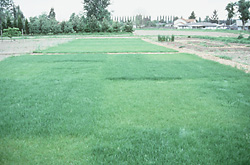
Imagine a situation in which we had just performed simple linear regression, and now we wished to summarize the trend graphically. For this demonstration, we will return to a dataset we used in a previous Workshop (the fertilizer data set): An agriculturalist was interested in the effects of fertilizer load on the yield of grass. Grass seed was sown uniformly over an area and different quantities of commercial fertilizer were applied to each of ten 1 m2 randomly located plots. Two months later the grass from each plot was harvested, dried and weighed. The data are in the file fertilizer.csv.Download Fertilizer data set
| Format of fertilizer.csv data files | |||||||||||||||||||
|---|---|---|---|---|---|---|---|---|---|---|---|---|---|---|---|---|---|---|---|
|
 |
||||||||||||||||||
> fert <- read.table("../downloads/data/fertilizer.csv", header = T,
+     sep = ",", strip.white = T)
> fert
   FERTILIZER YIELD
1          25    84
2          50    80
3          75    90
4         100   154
5         125   148
6         150   169
7         175   206
8         200   244
9         225   212
10        250   248
yi = β0 + βi x1 + εi |
|
εi ∼ Normal(0,σ2) |
#Residual 'random' effects |
> fert.lm <- lm(YIELD ~ FERTILIZER, data = fert)
> fert.lm
Call:
lm(formula = YIELD ~ FERTILIZER, data = fert)

Coefficients:
(Intercept)   FERTILIZER
     51.933        0.811
For example, if the estimated intercept (β0) and slope (β0) where 2 and 3 respectively, we could predict a new value of y when x was equal to 5.
yi = β0 + β1 xi |
yi = 2 + 3× xi |
y = 2 + 3× 5 |
y = 17 |
|
|
|
|
So what we are after is what is called the outer product of the two matrices. The outer product multiplies the first entry of the left matrix by the first value (first row) of the second matrix and the second values together and so on, and then sums them all up. In R, the outer product of two matrices is performed by the %*%.
> # Create a sequence of x-values that span the range of the Fertilizer
> #   variable
> coefs <- c(2, 3)
> cmat <- c(1, 5)
> coefs %*% cmat
     [,1]
[1,]   17
In this way, we can predict multiple new y values from multiple new x values. When the second matrix contains multiple columns, each column represents a separate contrast. Therefore the outer products are performed separately for each column of the second (contrast) matrix.
|
|
> # Create a sequence of x-values that span the range of the Fertilizer
> #   variable
> coefs <- c(2, 3)
> cmat <- cbind(c(1, 5), c(1, 5.5), c(1, 8))
> cmat
     [,1] [,2] [,3]
[1,]    1  1.0    1
[2,]    5  5.5    8
> coefs %*% cmat
     [,1] [,2] [,3]
[1,]   17 18.5   26
Use the predict() function to extract the line of best fit and standard errors
For simple examples such as this, there is a function called predict() that can be used to derive estimates (and standard errors) from simple linear models. This function is essentially a clever wrapper for the series of actions that we will perform manually. As it is well tested under simple conditions, it provides a good comparison and reference point for our manual calculations.
> # Create a sequence of x-values that span the range of the Fertilizer
> #   variable
> newX <- seq(min(fert$FERTILIZER), max(fert$FERTILIZER), l = 100)
> pred <- predict(fert.lm, newdata = data.frame(FERTILIZER = newX),
+     se = T)
> pred
$fit
     1      2      3      4      5      6      7      8      9     10     11     12     13     14
 72.22  74.06  75.91  77.75  79.59  81.44  83.28  85.13  86.97  88.81  90.66  92.50  94.35  96.19
    15     16     17     18     19     20     21     22     23     24     25     26     27     28
 98.04  99.88 101.72 103.57 105.41 107.26 109.10 110.94 112.79 114.63 116.48 118.32 120.16 122.01
    29     30     31     32     33     34     35     36     37     38     39     40     41     42
123.85 125.70 127.54 129.38 131.23 133.07 134.92 136.76 138.60 140.45 142.29 144.14 145.98 147.83
    43     44     45     46     47     48     49     50     51     52     53     54     55     56
149.67 151.51 153.36 155.20 157.05 158.89 160.73 162.58 164.42 166.27 168.11 169.95 171.80 173.64
    57     58     59     60     61     62     63     64     65     66     67     68     69     70
175.49 177.33 179.17 181.02 182.86 184.71 186.55 188.40 190.24 192.08 193.93 195.77 197.62 199.46
    71     72     73     74     75     76     77     78     79     80     81     82     83     84
201.30 203.15 204.99 206.84 208.68 210.52 212.37 214.21 216.06 217.90 219.74 221.59 223.43 225.28
    85     86     87     88     89     90     91     92     93     94     95     96     97     98
227.12 228.96 230.81 232.65 234.50 236.34 238.19 240.03 241.87 243.72 245.56 247.41 249.25 251.09
    99    100
252.94 254.78

$se.fit
     1      2      3      4      5      6      7      8      9     10     11     12     13     14
11.167 11.007 10.848 10.690 10.534 10.378 10.224 10.070  9.918  9.768  9.619  9.471  9.325  9.180
    15     16     17     18     19     20     21     22     23     24     25     26     27     28
 9.037  8.896  8.757  8.619  8.484  8.351  8.220  8.091  7.965  7.842  7.721  7.603  7.488  7.376
    29     30     31     32     33     34     35     36     37     38     39     40     41     42
 7.267  7.162  7.060  6.962  6.868  6.778  6.692  6.611  6.534  6.461  6.394  6.331  6.274  6.222
    43     44     45     46     47     48     49     50     51     52     53     54     55     56
 6.175  6.134  6.098  6.069  6.045  6.027  6.015  6.009  6.009  6.015  6.027  6.045  6.069  6.098
    57     58     59     60     61     62     63     64     65     66     67     68     69     70
 6.134  6.175  6.222  6.274  6.331  6.394  6.461  6.534  6.611  6.692  6.778  6.868  6.962  7.060
    71     72     73     74     75     76     77     78     79     80     81     82     83     84
 7.162  7.267  7.376  7.488  7.603  7.721  7.842  7.965  8.091  8.220  8.351  8.484  8.619  8.757
    85     86     87     88     89     90     91     92     93     94     95     96     97     98
 8.896  9.037  9.180  9.325  9.471  9.619  9.768  9.918 10.070 10.224 10.378 10.534 10.690 10.848
    99    100
11.007 11.167

$df
[1] 8

$residual.scale
[1] 19
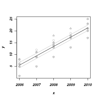
> plot(YIELD ~ FERTILIZER, fert, pch = 16)
> points(pred$fit ~ newX, type = "l")
> points(pred$fit - pred$se.fit ~ newX, type = "l", col = "grey")
> points(pred$fit + pred$se.fit ~ newX, type = "l", col = "grey")

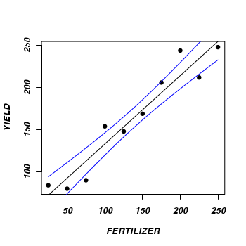
> #Now for 95% confidence intervals
> plot(YIELD ~ FERTILIZER, fert, pch = 16)
> points(pred$fit ~ newX, type = "l")
> lwrCI <- pred$fit + qnorm(0.025) * pred$se.fit
> uprCI <- pred$fit + qnorm(0.975) * pred$se.fit
> points(lwrCI ~ newX, type = "l", col = "blue")
> points(uprCI ~ newX, type = "l", col = "blue")
Use contrasts and matrix algebra to derive predictions and errors
- First retrieve the fitted model parameters (intercept and slope)
> coefs <- fert.lm$coef
> coefs
(Intercept) FERTILIZER 51.9333 0.8114 - Generate a model matrix appropriate for the predictor variable range.
The more numbers there are over the range the smoother (less jagged) the fitted curve.
Note that the contrast matrix that we just generated has the individual contrasts in rows whereas (recall) they need to be in columns. We can either transpose this matrix (with the t() function) and restore it, or else just use the t() function inline when calculating the outer product of the coefficients and contrast matrices.
> cc <- as.matrix(expand.grid(1, newX))
> head(cc)
     Var1  Var2
[1,]    1 25.00
[2,]    1 27.27
[3,]    1 29.55
[4,]    1 31.82
[5,]    1 34.09
[6,]    1 36.36
Essentially, what we want to do is:
yi =
×51.933 0.8114 1.000 1.000 1.000 ... 25.000 27.273 29.545 ... - Calculate (derive) the predicted yield values for each of the new Fertilizer concentrations.
> newY <- coefs %*% t(cc)
> newY
[,1] [,2] [,3] [,4] [,5] [,6] [,7] [,8] [,9] [,10] [,11] [,12] [,13] [,14] [,15] [1,] 72.22 74.06 75.91 77.75 79.59 81.44 83.28 85.13 86.97 88.81 90.66 92.5 94.35 96.19 98.04 [,16] [,17] [,18] [,19] [,20] [,21] [,22] [,23] [,24] [,25] [,26] [,27] [,28] [,29] [,30] [1,] 99.88 101.7 103.6 105.4 107.3 109.1 110.9 112.8 114.6 116.5 118.3 120.2 122 123.9 125.7 [,31] [,32] [,33] [,34] [,35] [,36] [,37] [,38] [,39] [,40] [,41] [,42] [,43] [,44] [,45] [1,] 127.5 129.4 131.2 133.1 134.9 136.8 138.6 140.4 142.3 144.1 146 147.8 149.7 151.5 153.4 [,46] [,47] [,48] [,49] [,50] [,51] [,52] [,53] [,54] [,55] [,56] [,57] [,58] [,59] [,60] [1,] 155.2 157 158.9 160.7 162.6 164.4 166.3 168.1 170 171.8 173.6 175.5 177.3 179.2 181 [,61] [,62] [,63] [,64] [,65] [,66] [,67] [,68] [,69] [,70] [,71] [,72] [,73] [,74] [,75] [1,] 182.9 184.7 186.6 188.4 190.2 192.1 193.9 195.8 197.6 199.5 201.3 203.1 205 206.8 208.7 [,76] [,77] [,78] [,79] [,80] [,81] [,82] [,83] [,84] [,85] [,86] [,87] [,88] [,89] [,90] [1,] 210.5 212.4 214.2 216.1 217.9 219.7 221.6 223.4 225.3 227.1 229 230.8 232.7 234.5 236.3 [,91] [,92] [,93] [,94] [,95] [,96] [,97] [,98] [,99] [,100] [1,] 238.2 240 241.9 243.7 245.6 247.4 249.2 251.1 252.9 254.8 - Calculate (derive) the standard errors of the predicted yield values for each of the new Fertilizer concentrations.
> vc <- vcov(fert.lm)
> se <- sqrt(diag(cc %*% vc %*% t(cc)))
> head(se)
[1] 11.17 11.01 10.85 10.69 10.53 10.38
- Reconstruct the summary plot with the derived fit, standard errors and confidence interval
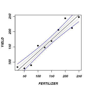
> plot(YIELD ~ FERTILIZER, fert, pch = 16)
> points(newY[1, ] ~ newX, type = "l")
> points(newY[1, ] - se ~ newX, type = "l", col = "grey")
> points(newY[1, ] + se ~ newX, type = "l", col = "grey")
> lwrCI <- newY[1, ] + qnorm(0.025) * se
> uprCI <- newY[1, ] + qnorm(0.975) * se
> points(lwrCI ~ newX, type = "l", col = "blue")
> points(uprCI ~ newX, type = "l", col = "blue")
Contrasts in linear mixed effects models
For the next demonstration, I will use completely fabricated data. Perhaps one day I will seek out a good example with real data, but for now, the artificial data will do.Create the artificial data
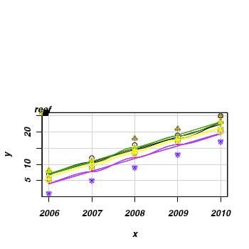
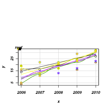
This data set consists of fish counts over time on seven reefs (you can tell it is artificial, because they have increased ;^)> set.seed(1) > x <- NULL > y <- NULL > for (i in 1:7) { + xx <- 2006:2010 + #yy <- round(3+2*x + rnorm(5,0,1) + rnorm(1,0,3),0)+1 + + yy <- round(-8300 + 4.14 * x + rnorm(5, 0, 1) + rnorm(1, 0, 3), 0) + 1 + yy[yy < 0] <- 0 + x <- c(x, xx) + y <- c(y, yy) + } > data <- data.frame(x, y, reef = gl(7, 5, 35, LETTERS[1:7])) > #use a scatterplot to explore the trend for each reef > library(car) > scatterplot(y ~ x | reef, data)
> library(MASS)
> data.lme <- glmmPQL(y ~ x, random = ~1 | reef, data, family = "gaussian")
> summary(data.lme)
Linear mixed-effects model fit by maximum likelihood
 Data: data
  AIC BIC logLik
   NA  NA     NA

Random effects:
 Formula: ~1 | reef
        (Intercept) Residual
StdDev:       1.362    1.744

Variance function:
 Structure: fixed weights
 Formula: ~invwt
Fixed effects: y ~ x
            Value Std.Error DF t-value p-value
(Intercept) -7875    244.02 97  -32.27       0
x               4      0.12 97   32.33       0
 Correlation:
  (Intr)
x -1

Standardized Within-Group Residuals:
    Min      Q1     Med      Q3     Max
-1.7777 -0.5180  0.1723  0.6385  1.8105

Number of Observations: 105
Number of Groups: 7
Use the predict() function to extract the line of best fit and standard errors
> # Create a sequence of x-values that span the range of the x variable
> newX <- seq(min(data$x), max(data$x), l = 100)
> pred <- predict(data.lme, newdata = data.frame(x = newX), level = 0,
+     se = T)
> pred
  [1]  5.543  5.702  5.860  6.019  6.178  6.337  6.495  6.654  6.813  6.971  7.130  7.289  7.448
 [14]  7.606  7.765  7.924  8.083  8.241  8.400  8.559  8.717  8.876  9.035  9.194  9.352  9.511
 [27]  9.670  9.829  9.987 10.146 10.305 10.463 10.622 10.781 10.940 11.098 11.257 11.416 11.575
 [40] 11.733 11.892 12.051 12.210 12.368 12.527 12.686 12.844 13.003 13.162 13.321 13.479 13.638
 [53] 13.797 13.956 14.114 14.273 14.432 14.590 14.749 14.908 15.067 15.225 15.384 15.543 15.702
 [66] 15.860 16.019 16.178 16.337 16.495 16.654 16.813 16.971 17.130 17.289 17.448 17.606 17.765
 [79] 17.924 18.083 18.241 18.400 18.559 18.717 18.876 19.035 19.194 19.352 19.511 19.670 19.829
 [92] 19.987 20.146 20.305 20.463 20.622 20.781 20.940 21.098 21.257
attr(,"label")
[1] "Predicted values"
Use contrasts and matrix algebra to derive predictions and errors
- First retrieve the fitted model parameters (intercept and slope) for the fixed effects.
> coefs <- data.lme$coef$fixed
> coefs
(Intercept)           x
  -7875.171       3.929
- Generate a model matrix appropriate for the predictor variable range.
The more numbers there are over the range the smoother (less jagged) the fitted curve.
> newX <- seq(2006, 2010, l = 100)
> cc <- as.matrix(expand.grid(1, newX))
> head(cc)
     Var1 Var2
[1,]    1 2006
[2,]    1 2006
[3,]    1 2006
[4,]    1 2006
[5,]    1 2006
[6,]    1 2006
- Calculate (derive) the predicted fish counts over time across all reefs.
> newY <- coefs %*% t(cc)
> newY
[,1] [,2] [,3] [,4] [,5] [,6] [,7] [,8] [,9] [,10] [,11] [,12] [,13] [,14] [,15] [,16] [1,] 5.543 5.702 5.86 6.019 6.178 6.337 6.495 6.654 6.813 6.971 7.13 7.289 7.448 7.606 7.765 7.924 [,17] [,18] [,19] [,20] [,21] [,22] [,23] [,24] [,25] [,26] [,27] [,28] [,29] [,30] [,31] [1,] 8.083 8.241 8.4 8.559 8.717 8.876 9.035 9.194 9.352 9.511 9.67 9.829 9.987 10.15 10.3 [,32] [,33] [,34] [,35] [,36] [,37] [,38] [,39] [,40] [,41] [,42] [,43] [,44] [,45] [,46] [1,] 10.46 10.62 10.78 10.94 11.1 11.26 11.42 11.57 11.73 11.89 12.05 12.21 12.37 12.53 12.69 [,47] [,48] [,49] [,50] [,51] [,52] [,53] [,54] [,55] [,56] [,57] [,58] [,59] [,60] [,61] [1,] 12.84 13 13.16 13.32 13.48 13.64 13.8 13.96 14.11 14.27 14.43 14.59 14.75 14.91 15.07 [,62] [,63] [,64] [,65] [,66] [,67] [,68] [,69] [,70] [,71] [,72] [,73] [,74] [,75] [,76] [1,] 15.23 15.38 15.54 15.7 15.86 16.02 16.18 16.34 16.5 16.65 16.81 16.97 17.13 17.29 17.45 [,77] [,78] [,79] [,80] [,81] [,82] [,83] [,84] [,85] [,86] [,87] [,88] [,89] [,90] [,91] [1,] 17.61 17.77 17.92 18.08 18.24 18.4 18.56 18.72 18.88 19.03 19.19 19.35 19.51 19.67 19.83 [,92] [,93] [,94] [,95] [,96] [,97] [,98] [,99] [,100] [1,] 19.99 20.15 20.3 20.46 20.62 20.78 20.94 21.1 21.26 - Calculate (derive) the standard errors of the predicted fish counts.
> vc <- vcov(data.lme)
> se <- sqrt(diag(cc %*% vc %*% t(cc)))
> head(se)
[1] 0.5931 0.5912 0.5893 0.5874 0.5855 0.5837
- Make a data frame to hold the predicted values, standard errors and confidence intervals
> mat <- data.frame(x = newX, fit = newY[1, ], se = se, lwr = newY[1,
+     ] + qnorm(0.025) * se, upr = newY[1, ] + qnorm(0.975) * se)
> head(mat)
     x   fit     se   lwr   upr
1 2006 5.543 0.5931 4.380 6.705
2 2006 5.702 0.5912 4.543 6.860
3 2006 5.860 0.5893 4.705 7.015
4 2006 6.019 0.5874 4.868 7.170
5 2006 6.178 0.5855 5.030 7.325
6 2006 6.337 0.5837 5.192 7.481
- Finally, lets plot the data with the predicted trend and confidence intervals overlaid
> plot(y ~ x, data, pch = as.numeric(data$reef), col = "grey")
> lines(fit ~ x, mat, col = "black")
> lines(lwr ~ x, mat, col = "grey")
> lines(upr ~ x, mat, col = "grey")
Contrasts in generalized linear mixed effects models
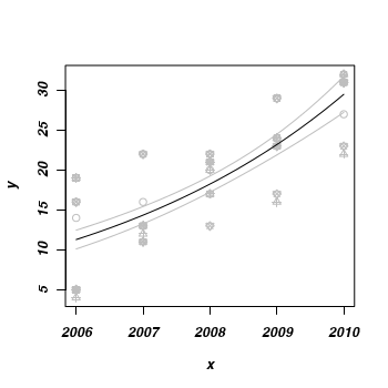
The next demonstration, will use very similar data to the previous example, except that a Poisson error distribution would be more appropriate (due to the apparent relationship between mean and variance).Create the artificial data
This data set consists of fish counts over time on seven reefs (you can tell it is artificial, because they have increased ;^)
> set.seed(2)
> x <- NULL
> y <- NULL
> for (i in 1:7) {
+     xx <- 2006:2010
+     yy <- round(-8300 + 4.14 * x + rpois(5, 2) * 2 + rnorm(1, 0, 3), 0) + 1
+     yy[yy < 0] <- 0
+     x <- c(x, xx)
+     y <- c(y, yy)
+ }
> data <- data.frame(x, y, reef = gl(7, 5, 35, LETTERS[1:7]))
> scatterplot(y ~ x | reef, data)
> hist(yy)

> #use a scatterplot to explore the trend for each reef
> library(car)
> scatterplot(y ~ x | reef, data)

> library(MASS)
> data.lme <- glmmPQL(y ~ x, random = ~1 | reef, data, family = "poisson")
> summary(data.lme)
Linear mixed-effects model fit by maximum likelihood
 Data: data
  AIC BIC logLik
   NA  NA     NA

Random effects:
 Formula: ~1 | reef
        (Intercept) Residual
StdDev:     0.02314    1.142

Variance function:
 Structure: fixed weights
 Formula: ~invwt
Fixed effects: y ~ x
             Value Std.Error DF t-value p-value
(Intercept) -479.6     37.74 97  -12.71       0
x              0.2      0.02 97   12.79       0
 Correlation:
  (Intr)
x -1

Standardized Within-Group Residuals:
    Min      Q1     Med      Q3     Max
-1.8834 -0.7651  0.1044  0.5940  2.0398

Number of Observations: 105
Number of Groups: 7
Use contrasts and matrix algebra to derive predictions and errors
- First retrieve the fitted model parameters (intercept and slope) for the fixed effects.
> coefs <- data.lme$coef$fixed
> coefs <- coefs
> coefs
(Intercept)           x
  -479.5766      0.2403
- Generate a model matrix appropriate for the predictor variable range.
The more numbers there are over the range the smoother (less jagged) the fitted curve.
> newX <- seq(2006, 2010, l = 100)
> cc <- as.matrix(expand.grid(1, newX))
> head(cc)
     Var1 Var2
[1,]    1 2006
[2,]    1 2006
[3,]    1 2006
[4,]    1 2006
[5,]    1 2006
[6,]    1 2006
- Calculate (derive) the predicted fish counts over time across all reefs.
As is, these will be on the log scale, since the canonical link function for a Poisson distribution is a log function.
Exponentiation will put this back in scale of the response (fish counts)
> newY <- exp(coefs %*% t(cc))
> newY
[,1] [,2] [,3] [,4] [,5] [,6] [,7] [,8] [,9] [,10] [,11] [,12] [,13] [,14] [,15] [,16] [1,] 11.28 11.39 11.5 11.62 11.73 11.84 11.96 12.08 12.19 12.31 12.43 12.55 12.68 12.8 12.92 13.05 [,17] [,18] [,19] [,20] [,21] [,22] [,23] [,24] [,25] [,26] [,27] [,28] [,29] [,30] [,31] [1,] 13.18 13.31 13.44 13.57 13.7 13.83 13.97 14.1 14.24 14.38 14.52 14.66 14.81 14.95 15.1 [,32] [,33] [,34] [,35] [,36] [,37] [,38] [,39] [,40] [,41] [,42] [,43] [,44] [,45] [,46] [1,] 15.24 15.39 15.54 15.69 15.85 16 16.16 16.32 16.48 16.64 16.8 16.96 17.13 17.29 17.46 [,47] [,48] [,49] [,50] [,51] [,52] [,53] [,54] [,55] [,56] [,57] [,58] [,59] [,60] [,61] [1,] 17.63 17.81 17.98 18.15 18.33 18.51 18.69 18.87 19.06 19.24 19.43 19.62 19.81 20.01 20.2 [,62] [,63] [,64] [,65] [,66] [,67] [,68] [,69] [,70] [,71] [,72] [,73] [,74] [,75] [,76] [1,] 20.4 20.6 20.8 21 21.21 21.41 21.62 21.83 22.05 22.26 22.48 22.7 22.92 23.14 23.37 [,77] [,78] [,79] [,80] [,81] [,82] [,83] [,84] [,85] [,86] [,87] [,88] [,89] [,90] [,91] [1,] 23.6 23.83 24.06 24.29 24.53 24.77 25.01 25.25 25.5 25.75 26 26.25 26.51 26.77 27.03 [,92] [,93] [,94] [,95] [,96] [,97] [,98] [,99] [,100] [1,] 27.29 27.56 27.83 28.1 28.38 28.65 28.93 29.21 29.5 - Calculate (derive) the standard errors of the predicted fish counts.
Again, these need to be corrected if they are to be on the response scale.
This is done by multiplying the standard error estimates by the exponential fitted estimates.
> vc <- vcov(data.lme)
> se <- sqrt(diag(cc %*% vc %*% t(cc)))
> se <- se * newY[1, ]
> head(se)
[1] 0.6003 0.5988 0.5972 0.5956 0.5939 0.5922
- Make a data frame to hold the predicted values, standard errors and confidence intervals
> mat <- data.frame(x = newX, fit = newY[1, ], se = se, lwr = newY[1,
+     ] + qnorm(0.025) * se, upr = newY[1, ] + qnorm(0.975) * se)
> head(mat)
     x   fit     se   lwr   upr
1 2006 11.28 0.6003 10.11 12.46
2 2006 11.39 0.5988 10.22 12.57
3 2006 11.50 0.5972 10.33 12.67
4 2006 11.62 0.5956 10.45 12.78
5 2006 11.73 0.5939 10.56 12.89
6 2006 11.84 0.5922 10.68 13.00
- Finally, lets plot the data with the predicted trend and confidence intervals overlaid
> plot(y ~ x, data, pch = as.numeric(data$reef), col = "grey")
> lines(fit ~ x, mat, col = "black")
> lines(lwr ~ x, mat, col = "grey")
> lines(upr ~ x, mat, col = "grey")
Contrasts in Single Factor ANOVA
Linear model effects parameterization for single factor ANOVA looks like:yi = μ + βi xi + εi |
|
εi ∼ Normal(0,σ2) |
#Residual 'random' effects |
Motivating example
Lets say we had measured a response (e.g. weight) from four individuals (replicates) treated in one of three ways (three treatment levels).
> set.seed(1)
> baseline <- 40
> all.effects <- c(baseline, 10, 15)
> sigma <- 3  #standard deviation
> n <- 3
> reps <- 4
> FactA <- gl(n = n, k = 4, len = n * reps, lab = paste("a", 1:n, sep = ""))
> X <- as.matrix(model.matrix(~FactA))
> eps <- round(rnorm(n * reps, 0, sigma), 2)
> Response <- as.numeric(as.matrix(X) %*% as.matrix(all.effects) +
+     eps)
> data <- data.frame(Response, FactA)
> write.table(data, file = "fish.csv", quote = F, row.names = F, sep = ",")
Download fish data set
> fish <- read.table("../downloads/data/fish.csv", header = T, sep = ",",
+     strip.white = T)
> fish
   Response FactA
1     38.12    a1
2     40.55    a1
3     37.49    a1
4     44.79    a1
5     50.99    a2
6     47.54    a2
7     51.46    a2
8     52.21    a2
9     56.73    a3
10    54.08    a3
11    59.54    a3
12    56.17    a3
| Raw data | Treatment means | ||||||||||||||
|---|---|---|---|---|---|---|---|---|---|---|---|---|---|---|---|
|
|
yi = μ + βi xi + εi |
|
y = μ + β1 x1 + β2 x2 + β3 x3 + εi |
# over-parameterized model |
y = β1 x1 + β2 x2 + β3 x3 + εi |
# means parameterization model |
y = Intercept + β2 x2 + β3 x3 + εi |
# effects parameterization model |
Two alternative model parameterizations (based on treatment contrasts) would be:
> # Means parameterization<br>
> data.frame(Response, FactA, model.matrix(~-1 + FactA, data = fish))
   Response FactA FactAa1 FactAa2 FactAa3
1     38.12    a1       1       0       0
2     40.55    a1       1       0       0
3     37.49    a1       1       0       0
4     44.79    a1       1       0       0
5     50.99    a2       0       1       0
6     47.54    a2       0       1       0
7     51.46    a2       0       1       0
8     52.21    a2       0       1       0
9     56.73    a3       0       0       1
10    54.08    a3       0       0       1
11    59.54    a3       0       0       1
12    56.17    a3       0       0       1
> # Effects parameterization<br>
> data.frame(Response, FactA, model.matrix(~FactA, data = fish))
   Response FactA X.Intercept. FactAa2 FactAa3
1     38.12    a1            1       0       0
2     40.55    a1            1       0       0
3     37.49    a1            1       0       0
4     44.79    a1            1       0       0
5     50.99    a2            1       1       0
6     47.54    a2            1       1       0
7     51.46    a2            1       1       0
8     52.21    a2            1       1       0
9     56.73    a3            1       0       1
10    54.08    a3            1       0       1
11    59.54    a3            1       0       1
12    56.17    a3            1       0       1
| Means parameterization | Effects parameterization | ||||||||||||||||||||||||||||||||||||||||||||||||||||||||||||||||||||||||||||||||||||||||||||||||||||||||||||||||||||||||||||||||||||||||||||
|---|---|---|---|---|---|---|---|---|---|---|---|---|---|---|---|---|---|---|---|---|---|---|---|---|---|---|---|---|---|---|---|---|---|---|---|---|---|---|---|---|---|---|---|---|---|---|---|---|---|---|---|---|---|---|---|---|---|---|---|---|---|---|---|---|---|---|---|---|---|---|---|---|---|---|---|---|---|---|---|---|---|---|---|---|---|---|---|---|---|---|---|---|---|---|---|---|---|---|---|---|---|---|---|---|---|---|---|---|---|---|---|---|---|---|---|---|---|---|---|---|---|---|---|---|---|---|---|---|---|---|---|---|---|---|---|---|---|---|---|---|---|
|
|
||||||||||||||||||||||||||||||||||||||||||||||||||||||||||||||||||||||||||||||||||||||||||||||||||||||||||||||||||||||||||||||||||||||||||||
Whilst the above two are equivalent for simple designs (such as that illustrated), the means parameterization (that does not include an intercept, or overall mean) is limited to simple single factor designs. Designs that involve additional predictors can only be accommodated via effects parameterization.
Lets now fit the above means and effects parameterized models and contrasts the estimated parameters:
| Means parameterization | Effects parameterization |
|---|---|
> summary(lm(Response ~ -1 + FactA, fish))$coef Estimate Std. Error t value Pr(>|t|) FactAa1 40.24 1.3 30.94 1.886e-10 FactAa2 50.55 1.3 38.87 2.453e-11 FactAa3 56.63 1.3 43.55 8.871e-12 |
> summary(lm(Response ~ FactA, fish))$coef Estimate Std. Error t value Pr(>|t|) (Intercept) 40.24 1.300 30.940 1.886e-10 FactAa2 10.31 1.839 5.607 3.312e-04 FactAa3 16.39 1.839 8.913 9.243e-06 |
The model on the left omits the intercept and thus estimates the treatment means. The parameters estimated by the model on the right are the mean of the first treatment level and the differences between each of the other treatment means and the first treatment mean. If there were only two treatment levels or first treatment was a control (two which you wish to compare the other treatment means), then the effects model is providing what the statisticians are advocating - estimates of the effect sizes as well as estimates of precision (standard error from which confidence intervals can easily be derived).
Derived parameters - simple contrasts
These parameters represent model coefficients that can be substituted back into a linear model. They represent the set of linear constants in the linear model. We can subsequently multiply these parameters to produce alternative linear combinations in order to estimate other values from the linear model.
yi = μ + βi xi |
yi = μ + β2 x2 + β2 x2 |
yi = 40.2375 × a1 + 10.3125 × a2 + 16.3925 × a3 |
|
|
The matrix;
|
yi = 40.2375 × a1 + 10.3125 × a2 + 16.3925 × a3 |
yi = 40.2375 × 0 + 10.3125 × 1 + 16.3925 × -1 |
yi = 10.3125 - 16.3925 |
yi = -6.080 |
Planned comparisons
Some researchers might be familiar with the use of contrasts in performing so called 'planned comparisons' or 'planned contrasts'. This involves redefining the actual parameters used in the linear model to reflect more meaningful comparisons amongst groups. For example, rather than compare each group mean against the mean of one (the first) treatment group, we many wish to include a comparison of the first treatment group (perhaps a control group) against the average two other treatment groups.
> contrasts(fish$FactA) <- cbind(`a1 vs (a2 & a3)` = c(1, -0.5, -0.5))
> summary(aov(Response ~ FactA, fish), split = list(FactA = list(1,
+     2)))
            Df Sum Sq Mean Sq F value  Pr(>F)
FactA        2    549     275    40.6 3.1e-05 ***
  FactA: C1  1    475     475    70.3 1.5e-05 ***
  FactA: C2  1     74      74    10.9  0.0091 **
Residuals    9     61       7
---
Signif. codes:  0 '***' 0.001 '**' 0.01 '*' 0.05 '.' 0.1 ' ' 1
> summary(aov(Response ~ FactA, fish), split = list(FactA = list(`a1 vs (a2 & a3)` = 1)))
                         Df Sum Sq Mean Sq F value  Pr(>F)
FactA                     2    549     275    40.6 3.1e-05 ***
  FactA: a1 vs (a2 & a3)  1    475     475    70.3 1.5e-05 ***
Residuals                 9     61       7
---
Signif. codes:  0 '***' 0.001 '**' 0.01 '*' 0.05 '.' 0.1 ' ' 1
> contrasts(fish$FactA) <- contr.treatment
> contrasts(fish$FactA) <- cbind(`a2 vs a3` = c(0, 1, -1))
> summary(aov(Response ~ FactA, fish), split = list(FactA = list(1,
+     2)))
            Df Sum Sq Mean Sq F value  Pr(>F)
FactA        2    549     275    40.6 3.1e-05 ***
  FactA: C1  1     74      74    10.9  0.0091 **
  FactA: C2  1    475     475    70.3 1.5e-05 ***
Residuals    9     61       7
---
Signif. codes:  0 '***' 0.001 '**' 0.01 '*' 0.05 '.' 0.1 ' ' 1
> summary(aov(Response ~ FactA, fish), split = list(FactA = list(`a2 vs a3` = 1)))
                  Df Sum Sq Mean Sq F value  Pr(>F)
FactA              2    549   274.7    40.6 3.1e-05 ***
  FactA: a2 vs a3  1     74    73.9    10.9  0.0091 **
Residuals          9     61     6.8
---
Signif. codes:  0 '***' 0.001 '**' 0.01 '*' 0.05 '.' 0.1 ' ' 1
> contrasts(fish$FactA) <- contr.treatment
In so doing, this technique provides a relatively easy way to test other non-standard hypotheses (linear effects).
However, a greater understanding of contrasts has even greater benefits when it comes to calculations of effect sizes, marginal means and their associated confidence intervals - features that are considered of greater interpretive value than hypothesis tests. Contrasts can also be used to derive a range of other derived parameters from the fitted model.
Calculating treatment means (and confidence intervals) from the effects model
A simple way to illustrate the use of contrasts to derive new parameters from a linear model is in the estimation of population treatment means from the effects model.
|
|
> contrasts(fish$FactA) <- contr.treatment
> fish.lm <- lm(Response ~ FactA, fish)
> cmat <- cbind(c(1, 0, 0), c(1, 1, 0), c(1, 0, 1))
> colnames(cmat) <- c("a1", "a2", "a3")
> fish.mu <- fish.lm$coef %*% cmat
> fish.mu
        a1    a2    a3
[1,] 40.24 50.55 56.63
> fish.se <- sqrt(diag(t(cmat) %*% vcov(fish.lm) %*% cmat))
> fish.se
 a1  a2  a3
1.3 1.3 1.3
> fish.ci <- as.numeric(fish.mu) + outer(fish.se, qt(c(0.025, 0.975),
+     df = fish.lm$df.resid))
> fish.ci
    [,1]  [,2]
a1 37.30 43.18
a2 47.61 53.49
a3 53.69 59.57
Calculating all the pairwise effects (and confidence intervals) from the effects model
|
|
> contrasts(data$FactA) <- contr.treatment
> data.lm <- lm(Response ~ FactA, data)
> cmat <- cbind(c(0, 1, 0), c(0, 0, 1), c(0, -1, 1))
> colnames(cmat) <- c("a1 vs a2", "a1 vs a3", "a2 vs a3")
> data.mu <- data.lm$coef %*% cmat
> data.mu
     a1 vs a2 a1 vs a3 a2 vs a3
[1,]    10.31    16.39     6.08
> data.se <- sqrt(diag(t(cmat) %*% vcov(data.lm) %*% cmat))
> data.se
a1 vs a2 a1 vs a3 a2 vs a3
   1.839    1.839    1.839
> data.ci <- as.numeric(data.mu) + outer(data.se, qt(c(0.025, 0.975),
+     df = data.lm$df.resid))
> data.ci
           [,1]  [,2]
a1 vs a2  6.152 14.47
a1 vs a3 12.232 20.55
a2 vs a3  1.920 10.24
Contrasts in factorial ANOVA
Motivating example
We now extend this example such that each individual fish was subjected to one of five levels of one treatment and one of three levels of another treatment. There were four replicate fish in each treatment combination.Note, this is an artificial data set. Most of the data sets used in this Workshop series have been real data sets. Real datasets are useful as they provide 'real world' examples of how to apply statistical principles and tools. However, for understanding some techniques, fabricated data allows us to explore techniques under controlled conditions. Furthermore, they allow us to compare statistical outcomes and patterns derived from statistical techniques to the 'truth'. Recall that the purpose of statistics is to 'estimate' population parameters. Fabricating data allows us to know the true values of the parameters that we are trying to estimate and thus allow us to evaluate the accuracy of our outcomes and understanding. I apologise if the use of artificial data causes you any pain or personal hardship.
In the creation of these data, I will be defining the 'true' (theoretical) effect sizes and level of 'noise'.
> set.seed(1)
> n.FactA <- 5
> n.FactB <- 3
> nsample <- 12
> n <- n.FactA * nsample
> #create factors
> FactA <- gl(n = n.FactA, k = nsample, length = n, lab = paste("a",
+     1:n.FactA, sep = ""))
> FactB <- gl(n = n.FactB, k = nsample/n.FactB, length = n, lab = paste("b",
+     1:n.FactB, sep = ""))
> #Effects
> baseline <- 40
> FactA.effects <- c(-10, -5, 5, 10)
> FactB.effects <- c(5, 10)
> interaction.effects <- c(-2, 3, 0, 4, 4, 0, 3, -2)
> all.effects <- c(baseline, FactA.effects, FactB.effects, interaction.effects)
> X <- as.matrix(model.matrix(~FactA * FactB))
Theoretical means
We will confirm the theoretical means of this design matrix (based on the defined effects).
> RESPONSE1 <- as.numeric(as.matrix(X) %*% as.matrix(all.effects))
> theoryMeans <- tapply(RESPONSE1, list(FactA, FactB), mean)
> theoryMeans
   b1 b2 b3
a1 40 45 50
a2 30 33 44
a3 35 43 45
a4 45 50 58
a5 50 59 58
> library(xtable)
> print(xtable(theoryMeans), type = "html", sanitize.rownames.function = function(x) paste("<b>",
+     x, "</b>"), html.table.attributes = list("border='3' cellpadding='5' cellspacing='0'"))
| b1 | b2 | b3 | |
|---|---|---|---|
| a1 | 40.00 | 45.00 | 50.00 |
| a2 | 30.00 | 33.00 | 44.00 |
| a3 | 35.00 | 43.00 | 45.00 |
| a4 | 45.00 | 50.00 | 58.00 |
| a5 | 50.00 | 59.00 | 58.00 |
And now we can add noise to the response to create data with variability. We will add noise by adding value to each observation that is randomly drawn from a normal distribution with a mean of zero and a standard deviation of 3.
> sigma <- 3
> eps <- rnorm(n, 0, sigma)
> X <- as.matrix(model.matrix(~FactA * FactB))
> RESPONSE <- as.numeric(as.matrix(X) %*% as.matrix(all.effects) +
+     eps)
> data <- data.frame(RESPONSE, FactB, FactA)
> write.table(data, file = "fish1.csv", quote = F, row.names = F, sep = ",")
Lets just examine the first six rows of these data to confirm that a little noise has been added
> head(data)
  RESPONSE FactB FactA
1    38.12    b1    a1
2    40.55    b1    a1
3    37.49    b1    a1
4    44.79    b1    a1
5    45.99    b2    a1
6    42.54    b2    a1
Download fish1 data set
> fish1 <- read.table("fish1.csv", header = T, sep = ",", strip.white = T)
> head(fish1)
  RESPONSE FactB FactA
1    38.12    b1    a1
2    40.55    b1    a1
3    37.49    b1    a1
4    44.79    b1    a1
5    45.99    b2    a1
6    42.54    b2    a1
Simple sample means
We will now calculate the sample means of each FactA by FactB combination. These are called 'cell means' as they are the means of each cell in a table in which the levels of FactA and FactB are the rows and columns (as was depicted in the table above for the theoretical means). If the samples are collected in an unbiased manner (whereby the collected samples reflect the populations), then the cell means should roughly approximate the true means of the underlying populations from whcih the observations were drawn.
Raw sample group means:> groupMeans <- with(fish1, tapply(RESPONSE, list(FactA, FactB), mean)) > groupMeans
      b1    b2    b3
a1 40.24 45.55 51.63
a2 28.68 34.76 43.84
a3 34.20 43.90 43.91
a4 46.06 50.63 57.80
a5 50.42 60.97 57.27
> theory_groupMeans <- theoryMeans - groupMeans
> theory_groupMeans
        b1      b2      b3
a1 -0.2376 -0.5511 -1.6290
a2  1.3170 -1.7571  0.1603
a3  0.7971 -0.8968  1.0936
a4 -1.0572 -0.6268  0.1974
a5 -0.4161 -1.9689  0.7325
Here is a side-by-side comparison of the theoretical means, the raw sample means and the cell differences:
| Theoretical cell means | Sample cell means | Differences | ||||||||||||||||||||||||||||||||||||||||||||||||||||||||||||||||||||||||
|---|---|---|---|---|---|---|---|---|---|---|---|---|---|---|---|---|---|---|---|---|---|---|---|---|---|---|---|---|---|---|---|---|---|---|---|---|---|---|---|---|---|---|---|---|---|---|---|---|---|---|---|---|---|---|---|---|---|---|---|---|---|---|---|---|---|---|---|---|---|---|---|---|---|---|
|
|
|
The sum of the deviations (differences) of the sample means from the theoretical means is:
> sum(theory_groupMeans)
[1] -4.843
Modeled population means
Alternatively, we can estimate the cell means based on a full multiplicative linear model.yij = µ + αi + βj + αβij
Note that this model is over-parameterized - that is, there are more parameters to estimate than there are groups of data from which to independently estimate them.
The effects parameterization of this model via treatment contrasts incorporates the mean of the first cell (µ) followed by a series of differences. In all, there are 15 groups (five levels of FactA multiplied by three levels of FactB) and correspondingly, there are 15 parameters being estimated:
yij = µ + β1 + β2 + β3 + β4 + β5 + β6 + β7 + β8 + β9 + β10 + β11 + β12 + β13 + β14
These parameters correspond to the following:
| Model term | Summarized model parameter (name given in R) | Interpretation |
|---|---|---|
| µ | (Intercept) | (a1b1) |
| β1 | FactAa2 | (a2b1 - a1b1) |
| β2 | FactAa3 | (a3b1 - a1b1) |
| β3 | FactAa4 | (a4b1 - a1b1) |
| β4 | FactAa5 | (a5b1 - a1b1) |
| β5 | FactBb2 | (a1b2 - a1b1) |
| β6 | FactBb3 | (a1b3 - a1b1) |
| β7 | FactAa2:FactBb2 | (a2b1+a1b2) - (a1b1+a2b2) |
| β8 | FactAa3:FactBb2 | (a3b1+a1b2) - (a1b1+a3b2) |
| β9 | FactAa4:FactBb2 | (a4b1+a1b2) - (a1b1+a4b2) |
| β10 | FactAa5:FactBb2 | (a5b1+a1b2) - (a1b1+a5b2) |
| β11 | FactAa2:FactBb3 | (a2b1+a1b3) - (a1b1+a2b3) |
| β12 | FactAa3:FactBb3 | (a3b1+a1b3) - (a1b1+a3b3) |
| β13 | FactAa4:FactBb3 | (a4b1+a1b3) - (a1b1+a4b3) |
| β14 | FactAa5:FactBb3 | (a5b1+a1b3) - (a1b1+a5b3) |
In R, the linear model is fitted via the lm() function.
> fish1.lm <- lm(RESPONSE ~ FactA * FactB, fish1)
Whilst these parameters satisfy the model parameterization, interpretating and utilizing the estimated parameters can take some getting used to. Lets begin by summarizing the estimates of the 15 model parameters.
> fish1.lm$coef
    (Intercept)         FactAa2         FactAa3         FactAa4         FactAa5         FactBb2
        40.2376        -11.5546         -6.0348          5.8196         10.1785          5.3135
        FactBb3 FactAa2:FactBb2 FactAa3:FactBb2 FactAa4:FactBb2 FactAa5:FactBb2 FactAa2:FactBb3
        11.3914          0.7606          4.3804         -0.7439          5.2393          3.7653
FactAa3:FactBb3 FactAa4:FactBb3 FactAa5:FactBb3
        -1.6879          0.3541         -4.5400
But this is where the good stuff begins. As the parameters are defined to encapsulate all of the patterns amongst the groups, the linear combination of parameters can now be used to calculate a whole range of related derived estimates (and their standard deviations etc) including:
- population cell means
- marginal means (row and column means)
- effect sizes (differences between marginal means)
- effect sizes (deviations from overall mean)
In order to achieve this wizardry, we must indicate which combination of the parameter estimates are relevant for each of the derived estimates required. And this is where contrast coefficients come in. The contrast coefficients are a set of numbers (equal in length to the number of model parameters) that determine the combinations and weights of the model parameters that are appropriate for each of the derived estimates. Hence when the set of model parameters are multiplied by a single set of contrast coefficients and then summed up, the result is a new derived estimate.
By way of example, the following contrast would specify that the derived estimate should include only (and all of) the first model parameter (and thus according to the table above, estimate the mean of cell FactA level a1 and FactB level b1). In R, the %*% is a special operator that performs matrix multiplication (each element of one matrix is multiplied by the corresponding elements of the other matrix) and returns their sum.
> fish1.lm$coef
    (Intercept)         FactAa2         FactAa3         FactAa4         FactAa5         FactBb2
        40.2376        -11.5546         -6.0348          5.8196         10.1785          5.3135
        FactBb3 FactAa2:FactBb2 FactAa3:FactBb2 FactAa4:FactBb2 FactAa5:FactBb2 FactAa2:FactBb3
        11.3914          0.7606          4.3804         -0.7439          5.2393          3.7653
FactAa3:FactBb3 FactAa4:FactBb3 FactAa5:FactBb3
        -1.6879          0.3541         -4.5400
> c(1, 0, 0, 0, 0, 0, 0, 0, 0, 0, 0, 0, 0, 0, 0)
[1] 1 0 0 0 0 0 0 0 0 0 0 0 0 0 0
> fish1.lm$coef %*% c(1, 0, 0, 0, 0, 0, 0, 0, 0, 0, 0, 0, 0, 0, 0)
      [,1]
[1,] 40.24
In the above, we indicated that only the first model parameter should be included in deriving the specified estimate, as all the others parameters are multiplied by zeros.
We can calculate multiple derived estimates at once, by multiplying the model parameters by multiple sets of contrast coefficients (represented as a matrix). That is, matrix multiplication. Hence to also calculate the cell mean of FactA level a2 and FactB b1 (a2b1), we would specify the first (a1b1 cell mean) and second (difference between a2b1 and a1b1 cell means) contrasts as ones (1) and the others zeros.
The cbind() function binds together vectors into the columns of a matrix.
> mat <- cbind(a1b1 = c(1, 0, 0, 0, 0, 0, 0, 0, 0, 0, 0, 0, 0, 0, 0),
+     a2b2 = c(1, 1, 0, 0, 0, 0, 0, 0, 0, 0, 0, 0, 0, 0, 0))
> mat
      a1b1 a2b2
 [1,]    1    1
 [2,]    0    1
 [3,]    0    0
 [4,]    0    0
 [5,]    0    0
 [6,]    0    0
 [7,]    0    0
 [8,]    0    0
 [9,]    0    0
[10,]    0    0
[11,]    0    0
[12,]    0    0
[13,]    0    0
[14,]    0    0
[15,]    0    0
> fish1.lm$coef %*% mat
      a1b1  a2b2
[1,] 40.24 28.68
At this point we could go on and attempt to work out which combinations of model parameters would be required to define each of the cell means. Whilst it is reasonably straight forward to do this for cells a1b1, a2b1, a3b1, a4b1, a5b1, a1b2, a1b3 (those along the top and down the left column), it requires more mental gymnastics to arrive at the entire set. However, there is a function in R called model.matrix() that helps us achieve this in a relatively pain-free manner. The model.matrix() function gives the design matrix that is used in linear modelling to indicate group membership of categorical variables and in general provides the link between the observed data (response) and the linear combination of predictor variables.
As just eluded to, model.matrix relates each individual observation. However, we are not interested in estimating ('predicting') each observation, we want to predict the means of groups of observations. Hence, we need to reduce the matrix down to the level of the groups.
> model.matrix(fish1.lm)
(Intercept) FactAa2 FactAa3 FactAa4 FactAa5 FactBb2 FactBb3 FactAa2:FactBb2 FactAa3:FactBb2 1 1 0 0 0 0 0 0 0 0 2 1 0 0 0 0 0 0 0 0 3 1 0 0 0 0 0 0 0 0 4 1 0 0 0 0 0 0 0 0 5 1 0 0 0 0 1 0 0 0 6 1 0 0 0 0 1 0 0 0 7 1 0 0 0 0 1 0 0 0 8 1 0 0 0 0 1 0 0 0 9 1 0 0 0 0 0 1 0 0 10 1 0 0 0 0 0 1 0 0 11 1 0 0 0 0 0 1 0 0 12 1 0 0 0 0 0 1 0 0 13 1 1 0 0 0 0 0 0 0 14 1 1 0 0 0 0 0 0 0 15 1 1 0 0 0 0 0 0 0 16 1 1 0 0 0 0 0 0 0 17 1 1 0 0 0 1 0 1 0 18 1 1 0 0 0 1 0 1 0 19 1 1 0 0 0 1 0 1 0 20 1 1 0 0 0 1 0 1 0 21 1 1 0 0 0 0 1 0 0 22 1 1 0 0 0 0 1 0 0 23 1 1 0 0 0 0 1 0 0 24 1 1 0 0 0 0 1 0 0 25 1 0 1 0 0 0 0 0 0 26 1 0 1 0 0 0 0 0 0 27 1 0 1 0 0 0 0 0 0 28 1 0 1 0 0 0 0 0 0 29 1 0 1 0 0 1 0 0 1 30 1 0 1 0 0 1 0 0 1 31 1 0 1 0 0 1 0 0 1 32 1 0 1 0 0 1 0 0 1 33 1 0 1 0 0 0 1 0 0 34 1 0 1 0 0 0 1 0 0 35 1 0 1 0 0 0 1 0 0 36 1 0 1 0 0 0 1 0 0 37 1 0 0 1 0 0 0 0 0 38 1 0 0 1 0 0 0 0 0 39 1 0 0 1 0 0 0 0 0 40 1 0 0 1 0 0 0 0 0 41 1 0 0 1 0 1 0 0 0 42 1 0 0 1 0 1 0 0 0 43 1 0 0 1 0 1 0 0 0 44 1 0 0 1 0 1 0 0 0 45 1 0 0 1 0 0 1 0 0 46 1 0 0 1 0 0 1 0 0 47 1 0 0 1 0 0 1 0 0 48 1 0 0 1 0 0 1 0 0 49 1 0 0 0 1 0 0 0 0 50 1 0 0 0 1 0 0 0 0 51 1 0 0 0 1 0 0 0 0 52 1 0 0 0 1 0 0 0 0 53 1 0 0 0 1 1 0 0 0 54 1 0 0 0 1 1 0 0 0 55 1 0 0 0 1 1 0 0 0 56 1 0 0 0 1 1 0 0 0 57 1 0 0 0 1 0 1 0 0 58 1 0 0 0 1 0 1 0 0 59 1 0 0 0 1 0 1 0 0 60 1 0 0 0 1 0 1 0 0 FactAa4:FactBb2 FactAa5:FactBb2 FactAa2:FactBb3 FactAa3:FactBb3 FactAa4:FactBb3 FactAa5:FactBb3 1 0 0 0 0 0 0 2 0 0 0 0 0 0 3 0 0 0 0 0 0 4 0 0 0 0 0 0 5 0 0 0 0 0 0 6 0 0 0 0 0 0 7 0 0 0 0 0 0 8 0 0 0 0 0 0 9 0 0 0 0 0 0 10 0 0 0 0 0 0 11 0 0 0 0 0 0 12 0 0 0 0 0 0 13 0 0 0 0 0 0 14 0 0 0 0 0 0 15 0 0 0 0 0 0 16 0 0 0 0 0 0 17 0 0 0 0 0 0 18 0 0 0 0 0 0 19 0 0 0 0 0 0 20 0 0 0 0 0 0 21 0 0 1 0 0 0 22 0 0 1 0 0 0 23 0 0 1 0 0 0 24 0 0 1 0 0 0 25 0 0 0 0 0 0 26 0 0 0 0 0 0 27 0 0 0 0 0 0 28 0 0 0 0 0 0 29 0 0 0 0 0 0 30 0 0 0 0 0 0 31 0 0 0 0 0 0 32 0 0 0 0 0 0 33 0 0 0 1 0 0 34 0 0 0 1 0 0 35 0 0 0 1 0 0 36 0 0 0 1 0 0 37 0 0 0 0 0 0 38 0 0 0 0 0 0 39 0 0 0 0 0 0 40 0 0 0 0 0 0 41 1 0 0 0 0 0 42 1 0 0 0 0 0 43 1 0 0 0 0 0 44 1 0 0 0 0 0 45 0 0 0 0 1 0 46 0 0 0 0 1 0 47 0 0 0 0 1 0 48 0 0 0 0 1 0 49 0 0 0 0 0 0 50 0 0 0 0 0 0 51 0 0 0 0 0 0 52 0 0 0 0 0 0 53 0 1 0 0 0 0 54 0 1 0 0 0 0 55 0 1 0 0 0 0 56 0 1 0 0 0 0 57 0 0 0 0 0 1 58 0 0 0 0 0 1 59 0 0 0 0 0 1 60 0 0 0 0 0 1 attr(,"assign") [1] 0 1 1 1 1 2 2 3 3 3 3 3 3 3 3 attr(,"contrasts") attr(,"contrasts")$FactA [1] "contr.treatment" attr(,"contrasts")$FactB [1] "contr.treatment"
- As the model contains only categorical predictors, we can just return a unique version (one without duplicates)
> mat <- unique(model.matrix(fish1.lm))
> head(mat)
   (Intercept) FactAa2 FactAa3 FactAa4 FactAa5 FactBb2 FactBb3 FactAa2:FactBb2 FactAa3:FactBb2
1            1       0       0       0       0       0       0               0               0
5            1       0       0       0       0       1       0               0               0
9            1       0       0       0       0       0       1               0               0
13           1       1       0       0       0       0       0               0               0
17           1       1       0       0       0       1       0               1               0
21           1       1       0       0       0       0       1               0               0
   FactAa4:FactBb2 FactAa5:FactBb2 FactAa2:FactBb3 FactAa3:FactBb3 FactAa4:FactBb3 FactAa5:FactBb3
1                0               0               0               0               0               0
5                0               0               0               0               0               0
9                0               0               0               0               0               0
13               0               0               0               0               0               0
17               0               0               0               0               0               0
21               0               0               1               0               0               0
- A more universal technique is to aggregate (summarize) the design matrix according to the factor levels. This technique also allows us to generate contrasts for marginal means and handles models that also include continuous covariates.
> # We take the design matrix converted into a data frame<br>
> # split the design matrix up into subsets according to the levels of FactA
> #   and FactB in the fish1 dataframe<br>
> # Apply the mean function to each column of these subsets<br>
> # Combine the means from each subset into a single data frame<br>
> # Retain all but the first two columns (which correspond to the the
> #   splitting variables that are appended<br>
> # onto the dataframe)<br>
> # It is then vitally important that the resulting dataframe be converted
> #   into a matrix to allow<br>
> # proper matrix multiplications<br>
> library(plyr)
> mat <- ddply(as.data.frame(model.matrix(fish1.lm)), ~fish1$FactA +
+     fish1$FactB, function(df) mean(df))[, -1:-2]
> mat <- as.matrix(mat)
> head(mat)
     (Intercept) FactAa2 FactAa3 FactAa4 FactAa5 FactBb2 FactBb3 FactAa2:FactBb2 FactAa3:FactBb2
[1,]           1       0       0       0       0       0       0               0               0
[2,]           1       0       0       0       0       1       0               0               0
[3,]           1       0       0       0       0       0       1               0               0
[4,]           1       1       0       0       0       0       0               0               0
[5,]           1       1       0       0       0       1       0               1               0
[6,]           1       1       0       0       0       0       1               0               0
     FactAa4:FactBb2 FactAa5:FactBb2 FactAa2:FactBb3 FactAa3:FactBb3 FactAa4:FactBb3
[1,]               0               0               0               0               0
[2,]               0               0               0               0               0
[3,]               0               0               0               0               0
[4,]               0               0               0               0               0
[5,]               0               0               0               0               0
[6,]               0               0               1               0               0
     FactAa5:FactBb3
[1,]               0
[2,]               0
[3,]               0
[4,]               0
[5,]               0
[6,]               0
Hence, the entire contrast matrix for deriving cell mean estimates would be (Note I will display this as transposed to make it more readable and to facilitate correct matrix multiplication).
> contrastMatrix <- t(mat)
> rownames(contrastMatrix) <- m1
> #nms<-unique(with(fish1,interaction(FactA,FactB,sep='')))
> #the following is safer as it is independent of the order of data in the
> #   data frame
> nms <- interaction(with(fish1, expand.grid(levels(FactB), levels(FactA))[,
+     c(2, 1)]), sep = "")
> #  with(fish1,expand.grid(levels(FactA),levels(FactB)))
> colnames(contrastMatrix) <- nms
> library(xtable)
> print(xtable(contrastMatrix), type = "html", sanitize.rownames.function = function(x) paste("<b>",
+     x, "</b>"), html.table.attributes = list("border='0' cellpadding='5' cellspacing='0'"))
| a1b1 | a1b2 | a1b3 | a2b1 | a2b2 | a2b3 | a3b1 | a3b2 | a3b3 | a4b1 | a4b2 | a4b3 | a5b1 | a5b2 | a5b3 | |
|---|---|---|---|---|---|---|---|---|---|---|---|---|---|---|---|
| µ | 1.00 | 1.00 | 1.00 | 1.00 | 1.00 | 1.00 | 1.00 | 1.00 | 1.00 | 1.00 | 1.00 | 1.00 | 1.00 | 1.00 | 1.00 |
| β1 | 0.00 | 0.00 | 0.00 | 1.00 | 1.00 | 1.00 | 0.00 | 0.00 | 0.00 | 0.00 | 0.00 | 0.00 | 0.00 | 0.00 | 0.00 |
| β2 | 0.00 | 0.00 | 0.00 | 0.00 | 0.00 | 0.00 | 1.00 | 1.00 | 1.00 | 0.00 | 0.00 | 0.00 | 0.00 | 0.00 | 0.00 |
| β3 | 0.00 | 0.00 | 0.00 | 0.00 | 0.00 | 0.00 | 0.00 | 0.00 | 0.00 | 1.00 | 1.00 | 1.00 | 0.00 | 0.00 | 0.00 |
| β4 | 0.00 | 0.00 | 0.00 | 0.00 | 0.00 | 0.00 | 0.00 | 0.00 | 0.00 | 0.00 | 0.00 | 0.00 | 1.00 | 1.00 | 1.00 |
| β5 | 0.00 | 1.00 | 0.00 | 0.00 | 1.00 | 0.00 | 0.00 | 1.00 | 0.00 | 0.00 | 1.00 | 0.00 | 0.00 | 1.00 | 0.00 |
| β6 | 0.00 | 0.00 | 1.00 | 0.00 | 0.00 | 1.00 | 0.00 | 0.00 | 1.00 | 0.00 | 0.00 | 1.00 | 0.00 | 0.00 | 1.00 |
| β7 | 0.00 | 0.00 | 0.00 | 0.00 | 1.00 | 0.00 | 0.00 | 0.00 | 0.00 | 0.00 | 0.00 | 0.00 | 0.00 | 0.00 | 0.00 |
| β8 | 0.00 | 0.00 | 0.00 | 0.00 | 0.00 | 0.00 | 0.00 | 1.00 | 0.00 | 0.00 | 0.00 | 0.00 | 0.00 | 0.00 | 0.00 |
| β9 | 0.00 | 0.00 | 0.00 | 0.00 | 0.00 | 0.00 | 0.00 | 0.00 | 0.00 | 0.00 | 1.00 | 0.00 | 0.00 | 0.00 | 0.00 |
| β10 | 0.00 | 0.00 | 0.00 | 0.00 | 0.00 | 0.00 | 0.00 | 0.00 | 0.00 | 0.00 | 0.00 | 0.00 | 0.00 | 1.00 | 0.00 |
| β11 | 0.00 | 0.00 | 0.00 | 0.00 | 0.00 | 1.00 | 0.00 | 0.00 | 0.00 | 0.00 | 0.00 | 0.00 | 0.00 | 0.00 | 0.00 |
| β12 | 0.00 | 0.00 | 0.00 | 0.00 | 0.00 | 0.00 | 0.00 | 0.00 | 1.00 | 0.00 | 0.00 | 0.00 | 0.00 | 0.00 | 0.00 |
| β13 | 0.00 | 0.00 | 0.00 | 0.00 | 0.00 | 0.00 | 0.00 | 0.00 | 0.00 | 0.00 | 0.00 | 1.00 | 0.00 | 0.00 | 0.00 |
| β14 | 0.00 | 0.00 | 0.00 | 0.00 | 0.00 | 0.00 | 0.00 | 0.00 | 0.00 | 0.00 | 0.00 | 0.00 | 0.00 | 0.00 | 1.00 |
The estimated population cell means are thence derived by multiplying the model parameters by this transposed contrast matrix (Note that the design matrix needs to be transposed such that the model parameters for each derived estimate are arranged into columns):
> fish1.lm$coef %*% t(mat)
      [,1]  [,2]  [,3]  [,4]  [,5]  [,6] [,7] [,8]  [,9] [,10] [,11] [,12] [,13] [,14] [,15]
[1,] 40.24 45.55 51.63 28.68 34.76 43.84 34.2 43.9 43.91 46.06 50.63  57.8 50.42 60.97 57.27
We can make the presentation of these numbers a little more palatable by arranging them in a table (matrix) and labeling the rows and columns.
> modelMeans <- matrix(fish1.lm$coef %*% t(mat), ncol = length(levels(fish1$FactB)),
+     byrow = T)
> dimnames(modelMeans) <- list(levels(fish1$FactA), levels(fish1$FactB))
> modelMeans
      b1    b2    b3
a1 40.24 45.55 51.63
a2 28.68 34.76 43.84
a3 34.20 43.90 43.91
a4 46.06 50.63 57.80
a5 50.42 60.97 57.27
Here is a side-by-side comparison of the theoretical means, the raw sample means and the cell differences:
| Theoretical cell means | Sample cell means | Model derived cell means | ||||||||||||||||||||||||||||||||||||||||||||||||||||||||||||||||||||||||
|---|---|---|---|---|---|---|---|---|---|---|---|---|---|---|---|---|---|---|---|---|---|---|---|---|---|---|---|---|---|---|---|---|---|---|---|---|---|---|---|---|---|---|---|---|---|---|---|---|---|---|---|---|---|---|---|---|---|---|---|---|---|---|---|---|---|---|---|---|---|---|---|---|---|---|
|
|
|
Although this might seem like a tedius way to calculate cell means, keep in mind that this is an example of a simple system. The same framework can be applied to more complex designs (such as nested, blocking, repeated measures - mixed effects models) for which simple sample means are unlikely to be as good at estimating true population means as estimates that are informed by all the FactA by Fact B trends across nesting levels. Furthermore, the model basis (and contrast sets) allows us to get estimates of standard deviations, standard errors and confidence intervals around the derived estimates.
Conditions
In order to make use of matrix algebra, the following formatting conditions must be adhered to:- the contrast matrix MUST be a matrix not a data frame
- Each column of the matrix represents a single separate derived parameter (contrasts are in columns)
- There must be exactly the same number of rows as there are parameters in the model
Standard deviations, standard errors and confidence intervals
Multiplying the contrast matrix by the model parameters derives new parameter estimates (as we have just seen). Multiplying the same contrast matrix by the model variance-covariance matrix derives estimates of the associated standard errors (and thus standard errors and confidence intervals). The variance-covariance matrix contains the variances of the estimated model parameters along the diagonals and the covariances between each parameter pair in the off-diagonals.
On a normal distribution, the mean plus or minus one standard deviation comprise approximately 68% of values. 95% of the data is encompassed by the span of data between the mean plus or minus approximately 2 standard deviations. To be more precise, the 95% of the data in a normal distribution span between the mean the following number of standard deviations:
> qnorm(c(0.025, 0.975))
[1] -1.96 1.96
Therefore, confidence intervals can be calculated from standard errors according to the following equation:
95% CI = μ ± 1.96 × SE |
Rather than produce the standard errors and confidence intervals in isolation, it is more useful to combine them into a frame along with the derived estimates (cell means in this case).
In the following code snippet, the function outer() multiplies each of the elements of one array with each of the elements of another array. This is called the outer product of the two arrays. In the code below, outer is used to multiply each of the standard error estimates by the upper and lower critical values for a 95% confidence interval from a normal distribution.
> modelMeans <- fish1.lm$coef %*% t(mat)
> se <- sqrt(diag(mat %*% vcov(fish1.lm) %*% t(mat)))
> #OR
> #se<-sqrt(diag(mat %*% tcrossprod(vcov(fish1.lm),mat)))
> ci <- as.numeric(modelMeans) + outer(se, qnorm(c(0.025, 0.975)))
> #OR
> #ci<-as.numeric(modelMeans)+outer(se,qt(df=45,c(.025,.975)))
> colnames(ci) <- c("lwr", "upr")
> mat2 <- cbind(mu = as.numeric(modelMeans), se = se, ci)
> rownames(mat2) <- nms
> #model.tables(aov(fish1.lm),type='means', se=T)
> mat2
        mu   se   lwr   upr
a1b1 40.24 1.35 37.59 42.88
a1b2 45.55 1.35 42.91 48.20
a1b3 51.63 1.35 48.98 54.27
a2b1 28.68 1.35 26.04 31.33
a2b2 34.76 1.35 32.11 37.40
a2b3 43.84 1.35 41.19 46.49
a3b1 34.20 1.35 31.56 36.85
a3b2 43.90 1.35 41.25 46.54
a3b3 43.91 1.35 41.26 46.55
a4b1 46.06 1.35 43.41 48.70
a4b2 50.63 1.35 47.98 53.27
a4b3 57.80 1.35 55.16 60.45
a5b1 50.42 1.35 47.77 53.06
a5b2 60.97 1.35 58.32 63.61
a5b3 57.27 1.35 54.62 59.91
There are a number of wrappers that can be used to perform the above sequence of functions. These include:
- predict() - most modelling functions have a predict() method. Unfortunately standard errors (and therefore confidence intervals) are only supplied for simple linear models.
- esticon() - in the doBy package. Given the model (lm, glm, lme) and the contrast matrix, this function will calculate the estimates and their standard errors (confidence intervals)
- popMeans() - also in the doBy package. Hence this is a convenient function for calculating population means (marginal or otherwise) from lm, glm and lme models (only).
As an example...
> library(doBy)
> popMeans(fish1.lm, c("FactB", "FactA"))
   beta0 Estimate Std.Error t.value DF Pr(>|t|) Lower Upper
1      0    40.24      1.35   29.81 45        0 37.52 42.96
2      0    45.55      1.35   33.74 45        0 42.83 48.27
3      0    51.63      1.35   38.24 45        0 48.91 54.35
4      0    28.68      1.35   21.25 45        0 25.96 31.40
5      0    34.76      1.35   25.75 45        0 32.04 37.48
6      0    43.84      1.35   32.47 45        0 41.12 46.56
7      0    34.20      1.35   25.34 45        0 31.48 36.92
8      0    43.90      1.35   32.52 45        0 41.18 46.62
9      0    43.91      1.35   32.52 45        0 41.19 46.63
10     0    46.06      1.35   34.12 45        0 43.34 48.78
11     0    50.63      1.35   37.50 45        0 47.91 53.35
12     0    57.80      1.35   42.82 45        0 55.08 60.52
13     0    50.42      1.35   37.35 45        0 47.70 53.14
14     0    60.97      1.35   45.16 45        0 58.25 63.69
15     0    57.27      1.35   42.42 45        0 54.55 59.99
Note, there is a slight difference between the confidence intervals that we calculated manually and those calculated by the popMeans() function. When we calculated the confidence intervals manually, we defined the 95% confidence intervals from a normal distribution. By contrast, the popMeans function defines the 95% confidence intervals from a t-distribution. For infinite degrees of freedom, the normal and t-distributions are identical. However, for smaller degrees of freedom (sample sizes), the t-distribution is relatively flatter and wider (and arguably a better reflection of the actual distribution). Consequently, the t-distribution might be considered to be more appropriate for models with small sample sizes.
Therefore, confidence intervals based on the t-distribution can be calculated from standard errors according to the following equation:
95% CI = μ ± t0.05,df × SE |
To achieve the same derived confidence intervals manually:
> mat <- unique(model.matrix(fish1.lm))
> modelMeans <- fish1.lm$coef %*% t(mat)
> se <- sqrt(diag(mat %*% vcov(fish1.lm) %*% t(mat)))
> ci <- as.numeric(modelMeans) + outer(se, qt(df = fish1.lm$df, c(0.025,
+     0.975)))
> colnames(ci) <- c("lwr", "upr")
> mat2 <- cbind(mu = as.numeric(modelMeans), se = se, ci)
> rownames(mat2) <- nms
> mat2
        mu   se   lwr   upr
a1b1 40.24 1.35 37.52 42.96
a1b2 45.55 1.35 42.83 48.27
a1b3 51.63 1.35 48.91 54.35
a2b1 28.68 1.35 25.96 31.40
a2b2 34.76 1.35 32.04 37.48
a2b3 43.84 1.35 41.12 46.56
a3b1 34.20 1.35 31.48 36.92
a3b2 43.90 1.35 41.18 46.62
a3b3 43.91 1.35 41.19 46.63
a4b1 46.06 1.35 43.34 48.78
a4b2 50.63 1.35 47.91 53.35
a4b3 57.80 1.35 55.08 60.52
a5b1 50.42 1.35 47.70 53.14
a5b2 60.97 1.35 58.25 63.69
a5b3 57.27 1.35 54.55 59.99
> #model.tables(aov(fish1.lm),type='means', se=T)
| mu | se | lwr | upr | |
|---|---|---|---|---|
| a1b1 | 40.24 | 1.35 | 37.52 | 42.96 |
| a1b2 | 45.55 | 1.35 | 42.83 | 48.27 |
| a1b3 | 51.63 | 1.35 | 48.91 | 54.35 |
| a2b1 | 28.68 | 1.35 | 25.96 | 31.40 |
| a2b2 | 34.76 | 1.35 | 32.04 | 37.48 |
| a2b3 | 43.84 | 1.35 | 41.12 | 46.56 |
| a3b1 | 34.20 | 1.35 | 31.48 | 36.92 |
| a3b2 | 43.90 | 1.35 | 41.18 | 46.62 |
| a3b3 | 43.91 | 1.35 | 41.19 | 46.63 |
| a4b1 | 46.06 | 1.35 | 43.34 | 48.78 |
| a4b2 | 50.63 | 1.35 | 47.91 | 53.35 |
| a4b3 | 57.80 | 1.35 | 55.08 | 60.52 |
| a5b1 | 50.42 | 1.35 | 47.70 | 53.14 |
| a5b2 | 60.97 | 1.35 | 58.25 | 63.69 |
| a5b3 | 57.27 | 1.35 | 54.55 | 59.99 |
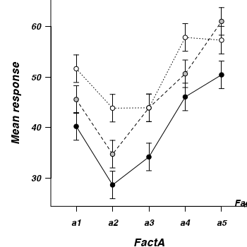
Interaction plot
If we add columns to this frame that indicate the levels of each of the factors, we can then create an interaction plot that incorporates confidence intervals in addition to the cell mean estimates.
> mat2 <- data.frame(with(fish1, expand.grid(FactB = levels(FactB),
+     FactA = levels(FactA))), mat2)
> mat2
     FactB FactA    mu   se   lwr   upr
a1b1    b1    a1 40.24 1.35 37.52 42.96
a1b2    b2    a1 45.55 1.35 42.83 48.27
a1b3    b3    a1 51.63 1.35 48.91 54.35
a2b1    b1    a2 28.68 1.35 25.96 31.40
a2b2    b2    a2 34.76 1.35 32.04 37.48
a2b3    b3    a2 43.84 1.35 41.12 46.56
a3b1    b1    a3 34.20 1.35 31.48 36.92
a3b2    b2    a3 43.90 1.35 41.18 46.62
a3b3    b3    a3 43.91 1.35 41.19 46.63
a4b1    b1    a4 46.06 1.35 43.34 48.78
a4b2    b2    a4 50.63 1.35 47.91 53.35
a4b3    b3    a4 57.80 1.35 55.08 60.52
a5b1    b1    a5 50.42 1.35 47.70 53.14
a5b2    b2    a5 60.97 1.35 58.25 63.69
a5b3    b3    a5 57.27 1.35 54.55 59.99
>
> par(mar = c(4, 5, 0, 0))
> lims <- with(mat2, range(c(lwr, upr)))
> plot(0, 0, xlim = c(0.5, 5.5), ylim = lims, type = "n", axes = F,
+     ann = F)
> #B1 series
> with(mat2[mat2$FactB == "b1", ], arrows(as.numeric(FactA), lwr, as.numeric(FactA),
+     upr, ang = 90, len = 0.05, code = 3))
> lines(mu ~ FactA, data = mat2[mat2$FactB == "b1", ], lty = 1)
> points(mu ~ FactA, data = mat2[mat2$FactB == "b1", ], pch = 21, bg = "black",
+     col = "black")
> #B2 series
> with(mat2[mat2$FactB == "b2", ], arrows(as.numeric(FactA), lwr, as.numeric(FactA),
+     upr, ang = 90, len = 0.05, code = 3))
> lines(mu ~ FactA, data = mat2[mat2$FactB == "b2", ], lty = 2)
> points(mu ~ FactA, data = mat2[mat2$FactB == "b2", ], pch = 21, bg = "grey",
+     col = "black")
> #B3 series
> with(mat2[mat2$FactB == "b3", ], arrows(as.numeric(FactA), lwr, as.numeric(FactA),
+     upr, ang = 90, len = 0.05, code = 3))
> lines(mu ~ FactA, data = mat2[mat2$FactB == "b3", ], lty = 3)
> points(mu ~ FactA, data = mat2[mat2$FactB == "b3", ], pch = 21, bg = "white",
+     col = "black")
> #axes
> axis(1, at = 1:5, lab = levels(mat2$FactA))
> mtext("FactA", 1, cex = 1.25, line = 3)
> axis(2, las = 1)
> mtext("Mean response", 2, cex = 1.25, line = 3)
> legend("bottomright", title = "FactB", leg = c("b1", "b2", "b3"),
+     bty = "n", lty = 1:3, pch = 21, pt.bg = c("black", "grey", "white"))
> box(bty = "l")
Unfortunately, for more complex designs (particularly those that are hierarchical), identifying or even approximating sensible estimates of degrees of freedom (and thus the t-distributions from which to estimate confidence intervals) becomes increasingly more problematic (and some argue, borders on quess work). As a result, more complex models do not provide any estimates of residual degrees of freedom and thus, it is necessary to either base confidence intervals on the normal distribution or provide your own degrees of freedom (and associated justification). Furthermore, as a result of these complications, the popMeans() function only supports models fitted via lm.
Marginal means
The true flexibility of the contrasts is the ability to derive other estimates, such as the marginal means for the levels of each of the factors. The contrasts for calculating marginal means are the average (averaged over the levels of the specific factor) contrast values for each parameter.
- FactA marginal means
> library(plyr)
> #mat <- model.matrix(~FactA*FactB,fish1)
> #dat <- cbind(fish1,mat)
> #FactA
> #cmat <- gsummary(dat,form=~FactA,base:::mean)
> cmat
     a1 vs a2 a1 vs a3 a2 vs a3
[1,]        0        0        0
[2,]        1        0       -1
[3,]        0        1        1
> cmat <- ddply(as.data.frame(model.matrix(fish1.lm)), ~fish1$FactA,
+     function(df) mean(df))
> class(cmat)
[1] "data.frame"
> # We need to convert this into a matrix and remove the first column (which
> #   was only used to help aggregate)<br>
> # We also need to transpose the matrix such that the contrasts are in
> #   columns rather than rows
> cmat <- t(as.matrix(cmat[, -1]))
> #cmat <- as.matrix(cmat[-1:-3])
> # Use this contrast matrix to derive new parameters and their standard
> #   errors
> FactAs <- fish1.lm$coef %*% cmat
> se <- sqrt(diag(t(cmat) %*% vcov(fish1.lm) %*% cmat))
> #ci<-as.numeric(FactAs)+outer(se,qnorm(c(.025,.975)))
> ci <- as.numeric(FactAs) + outer(se, qt(df = fish1.lm$df, c(0.025,
+     0.975)))
> colnames(ci) <- c("lwr", "upr")
> mat2 <- cbind(mu = as.numeric(FactAs), se, ci)
> rownames(mat2) <- levels(fish1$FactA)
Contrast matrix Marginal means 1 2 3 4 5 (Intercept) 1.00 1.00 1.00 1.00 1.00 FactAa2 0.00 1.00 0.00 0.00 0.00 FactAa3 0.00 0.00 1.00 0.00 0.00 FactAa4 0.00 0.00 0.00 1.00 0.00 FactAa5 0.00 0.00 0.00 0.00 1.00 FactBb2 0.33 0.33 0.33 0.33 0.33 FactBb3 0.33 0.33 0.33 0.33 0.33 FactAa2:FactBb2 0.00 0.33 0.00 0.00 0.00 FactAa3:FactBb2 0.00 0.00 0.33 0.00 0.00 FactAa4:FactBb2 0.00 0.00 0.00 0.33 0.00 FactAa5:FactBb2 0.00 0.00 0.00 0.00 0.33 FactAa2:FactBb3 0.00 0.33 0.00 0.00 0.00 FactAa3:FactBb3 0.00 0.00 0.33 0.00 0.00 FactAa4:FactBb3 0.00 0.00 0.00 0.33 0.00 FactAa5:FactBb3 0.00 0.00 0.00 0.00 0.33 
mu se lwr upr a1 45.81 0.78 44.24 47.38 a2 35.76 0.78 34.19 37.33 a3 40.67 0.78 39.10 42.24 a4 51.50 0.78 49.93 53.07 a5 56.22 0.78 54.65 57.79 - FactB marginal means
> #FactB
> cmat <- ddply(as.data.frame(model.matrix(fish1.lm)), ~fish1$FactB,
+     function(df) mean(df))
> cmat <- as.matrix(cmat[, -1])
> FactBs <- fish1.lm$coef %*% t(cmat)
> se <- sqrt(diag(cmat %*% vcov(fish1.lm) %*% t(cmat)))
> #ci<-as.numeric(FactBs)+outer(se,qnorm(c(.025,.975)))
> ci <- as.numeric(FactBs) + outer(se, qt(df = fish1.lm$df, c(0.025,
+     0.975)))
> colnames(ci) <- c("lwr", "upr")
> mat2 <- cbind(mu = as.numeric(FactBs), se, ci)
> rownames(mat2) <- levels(fish1$FactB)
Contrast matrix Marginal means 1 2 3 (Intercept) 1.00 1.00 1.00 FactAa2 0.20 0.20 0.20 FactAa3 0.20 0.20 0.20 FactAa4 0.20 0.20 0.20 FactAa5 0.20 0.20 0.20 FactBb2 0.00 1.00 0.00 FactBb3 0.00 0.00 1.00 FactAa2:FactBb2 0.00 0.20 0.00 FactAa3:FactBb2 0.00 0.20 0.00 FactAa4:FactBb2 0.00 0.20 0.00 FactAa5:FactBb2 0.00 0.20 0.00 FactAa2:FactBb3 0.00 0.00 0.20 FactAa3:FactBb3 0.00 0.00 0.20 FactAa4:FactBb3 0.00 0.00 0.20 FactAa5:FactBb3 0.00 0.00 0.20 mu se lwr upr b1 39.92 0.60 38.70 41.14 b2 47.16 0.60 45.94 48.38 b3 50.89 0.60 49.67 52.11 - FactA by FactB interaction marginal means (NOTE, as there are only two factors, this gives the marginal means of the highest order interaction - ie, the cell means)
> #FactA*FactB
> #As there are only two factors, below gives the marginal means of the
> #   highest order
> #interaction - ie, the cell means
> #cmat<-ddply(dat,~FactA*FactB,function(df) mean(df[,-1:-3]))
> cmat <- ddply(as.data.frame(model.matrix(fish1.lm)), ~fish1$FactA +
+     fish1$FactB, function(df) mean(df))
> cmat <- as.matrix(cmat[, -1:-2])
> FactAFactBs <- fish1.lm$coef %*% t(cmat)
> se <- sqrt(diag(cmat %*% vcov(fish1.lm) %*% t(cmat)))
> se <- sqrt(diag(cmat %*% vcov(fish1.lm) %*% t(cmat)))
> #ci<-as.numeric(FactAFactBs)+outer(se,qnorm(c(.025,.975)))
> ci <- as.numeric(FactAFactBs) + outer(se, qt(df = fish1.lm$df, c(0.025,
+     0.975)))
> colnames(ci) <- c("lwr", "upr")
> mat2 <- cbind(mu = as.numeric(FactAFactBs), se, ci)
> rownames(mat2) <- interaction(with(fish1, expand.grid(levels(FactB),
+     levels(FactA))[, c(2, 1)]), sep = "")
Contrast matrix 1 2 3 4 5 6 7 8 9 10 11 12 13 14 15 (Intercept) 1.00 1.00 1.00 1.00 1.00 1.00 1.00 1.00 1.00 1.00 1.00 1.00 1.00 1.00 1.00 FactAa2 0.00 0.00 0.00 1.00 1.00 1.00 0.00 0.00 0.00 0.00 0.00 0.00 0.00 0.00 0.00 FactAa3 0.00 0.00 0.00 0.00 0.00 0.00 1.00 1.00 1.00 0.00 0.00 0.00 0.00 0.00 0.00 FactAa4 0.00 0.00 0.00 0.00 0.00 0.00 0.00 0.00 0.00 1.00 1.00 1.00 0.00 0.00 0.00 FactAa5 0.00 0.00 0.00 0.00 0.00 0.00 0.00 0.00 0.00 0.00 0.00 0.00 1.00 1.00 1.00 FactBb2 0.00 1.00 0.00 0.00 1.00 0.00 0.00 1.00 0.00 0.00 1.00 0.00 0.00 1.00 0.00 FactBb3 0.00 0.00 1.00 0.00 0.00 1.00 0.00 0.00 1.00 0.00 0.00 1.00 0.00 0.00 1.00 FactAa2:FactBb2 0.00 0.00 0.00 0.00 1.00 0.00 0.00 0.00 0.00 0.00 0.00 0.00 0.00 0.00 0.00 FactAa3:FactBb2 0.00 0.00 0.00 0.00 0.00 0.00 0.00 1.00 0.00 0.00 0.00 0.00 0.00 0.00 0.00 FactAa4:FactBb2 0.00 0.00 0.00 0.00 0.00 0.00 0.00 0.00 0.00 0.00 1.00 0.00 0.00 0.00 0.00 FactAa5:FactBb2 0.00 0.00 0.00 0.00 0.00 0.00 0.00 0.00 0.00 0.00 0.00 0.00 0.00 1.00 0.00 FactAa2:FactBb3 0.00 0.00 0.00 0.00 0.00 1.00 0.00 0.00 0.00 0.00 0.00 0.00 0.00 0.00 0.00 FactAa3:FactBb3 0.00 0.00 0.00 0.00 0.00 0.00 0.00 0.00 1.00 0.00 0.00 0.00 0.00 0.00 0.00 FactAa4:FactBb3 0.00 0.00 0.00 0.00 0.00 0.00 0.00 0.00 0.00 0.00 0.00 1.00 0.00 0.00 0.00 FactAa5:FactBb3 0.00 0.00 0.00 0.00 0.00 0.00 0.00 0.00 0.00 0.00 0.00 0.00 0.00 0.00 1.00 
Marginal means mu se lwr upr a1b1 40.24 1.35 37.52 42.96 a1b2 45.55 1.35 42.83 48.27 a1b3 51.63 1.35 48.91 54.35 a2b1 28.68 1.35 25.96 31.40 a2b2 34.76 1.35 32.04 37.48 a2b3 43.84 1.35 41.12 46.56 a3b1 34.20 1.35 31.48 36.92 a3b2 43.90 1.35 41.18 46.62 a3b3 43.91 1.35 41.19 46.63 a4b1 46.06 1.35 43.34 48.78 a4b2 50.63 1.35 47.91 53.35 a4b3 57.80 1.35 55.08 60.52 a5b1 50.42 1.35 47.70 53.14 a5b2 60.97 1.35 58.25 63.69 a5b3 57.27 1.35 54.55 59.99
Again, for simple models, it is possible to use the popMeans function to get these marginal means:
> popMeans(fish1.lm, c("FactA"))
  beta0 Estimate Std.Error t.value DF Pr(>|t|) Lower Upper
1     0    45.81    0.7794   58.77 45        0 44.24 47.38
2     0    35.76    0.7794   45.88 45        0 34.19 37.33
3     0    40.67    0.7794   52.18 45        0 39.10 42.24
4     0    51.50    0.7794   66.07 45        0 49.93 53.07
5     0    56.22    0.7794   72.13 45        0 54.65 57.79
> popMeans(fish1.lm, c("FactB"))
  beta0 Estimate Std.Error t.value DF Pr(>|t|) Lower Upper
1     0    39.92    0.6037   66.12 45        0 38.70 41.14
2     0    47.16    0.6037   78.11 45        0 45.94 48.38
3     0    50.89    0.6037   84.29 45        0 49.67 52.11
Not surprisingly, for simple designs (like simple linear models), multiple bright members of the R community have written functions that derive the marginal means as well as the standard errors of the marginal mean effect sizes. This function is called model.tables().
> model.tables(aov(fish1.lm), type = "means", se = T)
Tables of means
Grand mean

45.99

 FactA
FactA
   a1    a2    a3    a4    a5
45.81 35.76 40.67 51.50 56.22

 FactB
FactB
   b1    b2    b3
39.92 47.16 50.89

 FactA:FactB
     FactB
FactA b1    b2    b3
   a1 40.24 45.55 51.63
   a2 28.68 34.76 43.84
   a3 34.20 43.90 43.91
   a4 46.06 50.63 57.80
   a5 50.42 60.97 57.27

Standard errors for differences of means
         FactA  FactB FactA:FactB
        1.1023 0.8538      1.9092
replic.     12     20           4
Effect sizes - differences between means
To derive effect sizes, you simply subtract one contrast set from another and use the result as the contrast for the derived parameter.
Effect sizes - for simple main effects
For example, to derive the effect size (difference between two parameters) of a1 vs a2 for the b1 level of Factor B:
THE NAMES IN THE CONTRAST MATRIX ARE NOT CORRECT> #mat <- unique(model.matrix(fish1.lm)) > mat <- ddply(as.data.frame(model.matrix(fish1.lm)), ~fish1$FactA + + fish1$FactB, function(df) mean(df)) > mat <- as.matrix(mat[, -1:-2]) > mat1 <- mat[1, ] - mat[4, ] > effectSizes <- fish1.lm$coef %*% mat1 > se <- sqrt(diag(mat1 %*% vcov(fish1.lm) %*% mat1)) > ci <- as.numeric(effectSizes) + outer(se, qt(df = fish1.lm$df, c(0.025, + 0.975))) > colnames(ci) <- c("lwr", "upr") > mat2 <- cbind(mu = as.numeric(effectSizes), se = se, ci) > mat2
        mu    se   lwr  upr
[1,] 11.55 1.909 7.709 15.4
| Contrast matrix for cell | Contrast matrix for | Effect size for | ||||||||||||||||||||||||||||||||||||||||||||||||||||||||||||||||||||||||||||||||||||||||||||
|---|---|---|---|---|---|---|---|---|---|---|---|---|---|---|---|---|---|---|---|---|---|---|---|---|---|---|---|---|---|---|---|---|---|---|---|---|---|---|---|---|---|---|---|---|---|---|---|---|---|---|---|---|---|---|---|---|---|---|---|---|---|---|---|---|---|---|---|---|---|---|---|---|---|---|---|---|---|---|---|---|---|---|---|---|---|---|---|---|---|---|---|---|---|---|
| means (a1b1 & a2b1) | a1b1 - a2b1 | a1b1 - a2b1 | ||||||||||||||||||||||||||||||||||||||||||||||||||||||||||||||||||||||||||||||||||||||||||||
|
minus |
|
equals |
|
Whilst it is possible to go through and calculate all the rest of the effects individually, we can loop through and create a matrix that contains all the appropriate contrasts.
Effect sizes - for marginal effects (no interactions)
Effect sizes of FactA marginal means
> #cmat<-ddply(dat,~FactA,function(df) mean(df[,-1:-3]))
> cmat <- ddply(as.data.frame(model.matrix(fish1.lm)), ~fish1$FactA,
+     function(df) mean(df))
>
> cmat <- as.matrix(cmat[, -1])
> #fish1.lm$coef %*% c(0,1,0,0,0,0,0,1/3,0,0,0,1/3,0,0,0)
> cm <- NULL
> for (i in 1:(nrow(cmat) - 1)) {
+     for (j in (i + 1):nrow(cmat)) {
+         nm <- paste(levels(fish1$FactA)[j], "-", levels(fish1$FactA)[i])
+         eval(parse(text = paste("cm <- cbind(cm,'", nm, "'=c(cmat[j,]-cmat[i,]))")))
+     }
+ }
> FactAEffects <- fish1.lm$coef %*% cm
> se <- sqrt(diag(t(cm) %*% vcov(fish1.lm) %*% cm))
> ci <- as.numeric(FactAEffects) + outer(se, qnorm(c(0.025, 0.975)))
> colnames(ci) <- c("lwr", "upr")
> mat2 <- cbind(mu = as.numeric(FactAEffects), se, ci)
| Contrast matrix | ||||||||||||||||||||||||||||||||||||||||||||||||||||||||||||||||||||||||||||||||||||||||||||||||||||||||||||||||||||||||||||||||||||||||||||||||||||||||||||||||||||||||||||||||
|---|---|---|---|---|---|---|---|---|---|---|---|---|---|---|---|---|---|---|---|---|---|---|---|---|---|---|---|---|---|---|---|---|---|---|---|---|---|---|---|---|---|---|---|---|---|---|---|---|---|---|---|---|---|---|---|---|---|---|---|---|---|---|---|---|---|---|---|---|---|---|---|---|---|---|---|---|---|---|---|---|---|---|---|---|---|---|---|---|---|---|---|---|---|---|---|---|---|---|---|---|---|---|---|---|---|---|---|---|---|---|---|---|---|---|---|---|---|---|---|---|---|---|---|---|---|---|---|---|---|---|---|---|---|---|---|---|---|---|---|---|---|---|---|---|---|---|---|---|---|---|---|---|---|---|---|---|---|---|---|---|---|---|---|---|---|---|---|---|---|---|---|---|---|---|---|---|
|
||||||||||||||||||||||||||||||||||||||||||||||||||||||||||||||||||||||||||||||||||||||||||||||||||||||||||||||||||||||||||||||||||||||||||||||||||||||||||||||||||||||||||||||||
| Marginal means | ||||||||||||||||||||||||||||||||||||||||||||||||||||||||||||||||||||||||||||||||||||||||||||||||||||||||||||||||||||||||||||||||||||||||||||||||||||||||||||||||||||||||||||||||
|
Effect sizes plot
> plot(seq(-22, 22, l = nrow(mat2)), 1:nrow(mat2), type = "n", ann = F,
+     axes = F)
> abline(v = 0, lty = 2)
> segments(mat2[, "lwr"], 1:nrow(mat2), mat2[, "upr"], 1:nrow(mat2))
> points(mat2[, "mu"], 1:nrow(mat2), pch = 16)
> text(mat2[, "lwr"], 1:nrow(mat2), lab = rownames(mat2), pos = 2)
> #text(mat2[,'mu'],1:nrow(mat2),lab=rownames(mat2), pos=1)
> axis(1)

Effect sizes of FactB marginal means
> #cmat<-ddply(dat,~FactB,function(df) mean(df[,-1:-3]))
> cmat <- ddply(as.data.frame(model.matrix(fish1.lm)), ~fish1$FactB,
+     function(df) mean(df))
> cmat <- as.matrix(cmat[, -1])
> #fish1.lm$coef %*% c(0,1,0,0,0,0,0,1/3,0,0,0,1/3,0,0,0)
> cm <- NULL
> for (i in 1:(nrow(cmat) - 1)) {
+     for (j in (i + 1):nrow(cmat)) {
+         nm <- paste(levels(fish1$FactB)[j], "-", levels(fish1$FactB)[i])
+         eval(parse(text = paste("cm <- cbind(cm,'", nm, "'=c(cmat[j,]-cmat[i,]))")))
+         #print(fish1.lm$coef %*% c(cmat[j,]-cmat[i,]))
+     }
+ }
> FactBEffects <- fish1.lm$coef %*% cm
> se <- sqrt(diag(t(cm) %*% vcov(fish1.lm) %*% cm))
> ci <- as.numeric(FactBEffects) + outer(se, qnorm(c(0.025, 0.975)))
> colnames(ci) <- c("lwr", "upr")
> mat2 <- cbind(mu = as.numeric(FactBEffects), se, ci)
| Contrast matrix | ||||||||||||||||||||||||||||||||||||||||||||||||||||||||||||||||
|---|---|---|---|---|---|---|---|---|---|---|---|---|---|---|---|---|---|---|---|---|---|---|---|---|---|---|---|---|---|---|---|---|---|---|---|---|---|---|---|---|---|---|---|---|---|---|---|---|---|---|---|---|---|---|---|---|---|---|---|---|---|---|---|---|
|
||||||||||||||||||||||||||||||||||||||||||||||||||||||||||||||||
| Marginal means | ||||||||||||||||||||||||||||||||||||||||||||||||||||||||||||||||
|
Simple main effects - effects associated with one factor at specific levels of another factor
But what do we do in the presence of an interaction then - when effect sizes of marginal means will clearly be underrepresenting the patterns. The presence of an interaction implies that the effect sizes differ according to the combinations of the factor levels.
For example, lets explore the effects of b1 vs b3 at each of the levels of Factor A
> fits <- NULL
> for (fA in levels(fish1$FactA)) {
+     mat <- model.matrix(~FactA * FactB, fish1[fish1$FactA == fA & fish1$FactB %in%
+         c("b1", "b3"), ])
+     mat <- unique(mat)
+     dat <- fish1[fish1$FactA == fA & fish1$FactB %in% c("b1", "b3"), ]
+     dat$FactB <- factor(dat$FactB)
+     cm <- NULL
+     for (i in 1:(nrow(mat) - 1)) {
+         for (j in (i + 1):nrow(mat)) {
+             nm <- with(dat, paste(levels(FactB)[j], "-", levels(FactB)[i]))
+             eval(parse(text = paste("cm <- cbind(cm,'", nm, "'=c(mat[j,]-mat[i,]))")))
+         }
+     }
+     es <- fish1.lm$coef %*% cm
+     se <- sqrt(diag(t(cm) %*% vcov(fish1.lm) %*% cm))
+     ci <- as.numeric(es) + outer(se, qnorm(c(0.025, 0.975)))
+     mat2 <- cbind(mu = as.numeric(es), se, ci)
+     fits <- rbind(fits, mat2)
+ }
> colnames(fits) <- c("ES", "se", "lwr", "upr")
> rname <- rownames(fits)
> fits <- data.frame(fits)
> fits$FactA <- levels(fish1$FactA)
> fits$Comp <- factor(rname)
> #fits
> fits <- NULL
> for (fA in levels(fish1$FactA)) {
+     cc <- combn(levels(fish1$FactB), 2)
+     for (nfb in 1:ncol(cc)) {
+         dat <- fish1[fish1$FactA == fA & fish1$FactB %in% cc[, nfb], ]
+         mat <- model.matrix(~FactA * FactB, fish1 = dat)
+         mat <- unique(mat)
+         dat$FactB <- factor(dat$FactB)
+         cm <- NULL
+         for (i in 1:(nrow(mat) - 1)) {
+             for (j in (i + 1):nrow(mat)) {
+                 nm <- with(dat, paste(levels(FactB)[j], "-", levels(FactB)[i]))
+                 eval(parse(text = paste("cm <- cbind(cm,'", nm, "'=c(mat[j,]-mat[i,]))")))
+             }
+         }
+         es <- fish1.lm$coef %*% cm
+         se <- sqrt(diag(t(cm) %*% vcov(fish1.lm) %*% cm))
+         ci <- as.numeric(es) + outer(se, qnorm(c(0.025, 0.975)))
+         mat2 <- cbind(mu = as.numeric(es), se, ci, fA)
+         mat2 <- data.frame(mu = as.numeric(es), se, ci, fA, Comp = rownames(mat2))
+         fits <- rbind(fits, mat2)
+     }
+ }
> colnames(fits) <- c("ES", "se", "lwr", "upr", "FactA", "Comp")
> #fits
> #predicted from marginal means
> oo <- outer(FactAs, FactBs, FUN = "+")/2
>
> dat <- fish1[fish1$FactA %in% levels(fish1$FactA) & fish1$FactB ==
+     "b1", ]
> mat <- unique(model.matrix(~FactA * FactB, fish1 = dat))
> fish1.lm$coef %*% t(mat)
         1     5     9    13    17    21   25   29    33    37    41   45    49    53    57
[1,] 40.24 45.55 51.63 28.68 34.76 43.84 34.2 43.9 43.91 46.06 50.63 57.8 50.42 60.97 57.27