Workshop 11.2b - χ2 tests (Bayesian)
23 April 2011
Basic χ2 references
- Logan (2010) - Chpt 16-17
- Quinn & Keough (2002) - Chpt 13-14
View R code for preliminaries.
> library(R2jags)
> library(ggplot2)
> library(grid)
> libray(coda)
Error: could not find function "libray"
>
> #define my common ggplot options
> murray_opts <- opts(panel.grid.major=theme_blank(),
+ 			   panel.grid.minor=theme_blank(),
+ 			   panel.border = theme_blank(),
+ 			   panel.background = theme_blank(),
+ 			   axis.title.y=theme_text(size=15, vjust=0,angle=90),
+ 			   axis.text.y=theme_text(size=12),
+ 			   axis.title.x=theme_text(size=15, vjust=-1),
+ 			   axis.text.x=theme_text(size=12),
+ 			   axis.line = theme_segment(),
+ 			   legend.position=c(1,0.1),legend.justification=c(1,0),
+ 			   legend.key=theme_blank(),
+ 			   plot.margin=unit(c(0.5,0.5,1,2),"lines")
+ )
Goodness of fit test
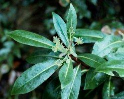
A fictitious plant ecologist sampled 90 shrubs of a dioecious plant in a forest, and each plant was classified as being either male or female. The ecologist was interested in the sex ratio and whether it differed from 50:50. The observed counts and the predicted (expected) counts based on a theoretical 50:50 sex ratio follow.
| Format of fictitious plant sex ratios - note, not a file | |||||||||||||
|---|---|---|---|---|---|---|---|---|---|---|---|---|---|
Expected and Observed data (50:50 sex ratio).
|
 |
Note, it is not necessary to open or create a data file for this question.
- As the fictitious researcher was interested in exploring sex parity (1:1 frequency ratio) in the dioecious plant,
the $\chi^2$ statistic would seem appropriate. Recall that the $\chi^2$ statistic is defined as:
$$\chi^2=\sum\frac{(o-e)^2}{e}$$
In effect, the chi-square statistic (which incorporates the variability in the data in to measure of the difference between observed and expected)
becomes the input for the likelihood model. Whilst we could simply pass JAGS the chi-square statistic, by
parsing the observed and expected values and having the chi-square value calculated within JAGS data,
the resulting JAGS code is more complete and able to accommodate other scenarios.
So if, $chisq$ is the chi-square statistic and $k$ is the degrees of freedom (and thus expected value of the $\chi^2$ distribution), then the likelihood model is:
\begin{align*} chisq &\sim \chi^2(k)\\ k &\sim U(0.01, 100) \end{align*} Translate this into JAGS code.Show code> modelString=" + data { + for (i in 1:n){ + resid[i] <- pow(obs[i]-exp[i],2)/exp[i] + } + chisq <- sum(resid) + } + model { + #Likelihood + chisq ~ dchisqr(k) + k ~ dunif(0.01,100) + } + " > ## write the model to a text file (I suggest you alter the path to somewhere more relevant > ## to your system!) > writeLines(modelString,con="../downloads/BUGSscripts/ws11.2bQ1.1.txt") -
We can now generate the observed and expected data as a list (as is necessary for JAGS).
When exploring parity, we are "expecting" the number of Females and Males to be very similar.
So from 90 individuals we expect 50% (0.5) to be Female and 50% to be Male.
To supply the JAGS code created in the step above, we require the observed counts, expected counts
and the number of classification levels ($=2$, Females and Males).
Show code
> #The observed Female and Male plant frequencies
> obs <- c(40, 50)
> #The expected Female and Make plant frequencies
> exp <- rep(sum(obs) * 0.5, 2)
> plant.list <- list(obs = c(40, 50), exp = exp, n = 2)
> plant.list
$obs
[1] 40 50

$exp
[1] 45 45

$n
[1] 2
- Next we should define the behavioural parameters of the MCMC sampling chains.
Include the following:
- the nodes (estimated parameters) to monitor (return samples for)
- the number of MCMC chains (3)
- the number of burnin steps (1000)
- the thinning factor (10)
- the number of MCMC iterations - determined by the number of samples to save, the rate of thinning and the number of chains
Show code> params <- c("chisq", "resid", "k") > nChains = 3 > burnInSteps = 1000 > thinSteps = 10 > numSavedSteps = 5000 > nIter = ceiling((numSavedSteps * thinSteps)/nChains)
- Now run the JAGS code via the R2jags interface and view a summary.
Show code
> #Run any random function just to get .Random.seed started
> runif(1)
[1] 0.1886
> plant.r2jags <- jags(data = plant.list, inits = NULL, parameters.to.save = params,
+     model.file = "../downloads/BUGSscripts/ws11.2bQ1.1.txt", n.chains = 3, n.iter = nIter,
+     n.burnin = burnInSteps, n.thin = thinSteps)
Compiling data graph
   Resolving undeclared variables
   Allocating nodes
   Initializing
   Reading data back into data table
Compiling model graph
   Resolving undeclared variables
   Allocating nodes
   Graph Size: 11

Initializing model
> print(plant.r2jags)Inference for Bugs model at "../downloads/BUGSscripts/ws11.2bQ1.1.txt", fit using jags, 3 chains, each with 16667 iterations (first 1000 discarded), n.thin = 10 n.sims = 4701 iterations saved mu.vect sd.vect 2.5% 25% 50% 75% 97.5% Rhat n.eff chisq 1.111 0.000 1.111 1.111 1.111 1.111 1.111 1.000 1 k 2.880 1.620 0.505 1.663 2.623 3.826 6.609 1.001 4700 resid[1] 0.556 0.000 0.556 0.556 0.556 0.556 0.556 1.000 1 resid[2] 0.556 0.000 0.556 0.556 0.556 0.556 0.556 1.000 1 deviance 3.453 1.379 2.498 2.592 2.921 3.769 7.202 1.002 1700 For each parameter, n.eff is a crude measure of effective sample size, and Rhat is the potential scale reduction factor (at convergence, Rhat=1). DIC info (using the rule, pD = var(deviance)/2) pD = 1.0 and DIC = 4.4 DIC is an estimate of expected predictive error (lower deviance is better). - Prior to using the MCMC samples, we should confirm that the chains converged on a stable
posterior distribution with adequate mixing (note it is really only k that we are interested in):
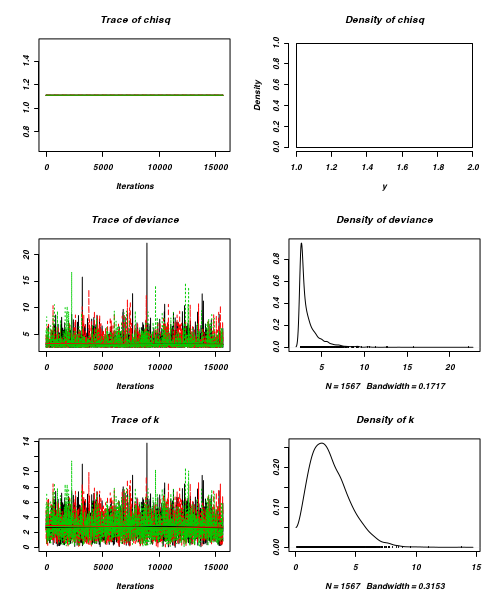
- Trace and density plots
View codeConclusion:
> plot(as.mcmc(plant.r2jags))

- Raftery diagnostic
View codeConclusion:
> raftery.diag(as.mcmc(plant.r2jags))
[[1]]

Quantile (q) = 0.025
Accuracy (r) = +/- 0.005
Probability (s) = 0.95

You need a sample size of at least 3746 with these values of q, r and s

[[2]]

Quantile (q) = 0.025
Accuracy (r) = +/- 0.005
Probability (s) = 0.95

You need a sample size of at least 3746 with these values of q, r and s

[[3]]

Quantile (q) = 0.025
Accuracy (r) = +/- 0.005
Probability (s) = 0.95

You need a sample size of at least 3746 with these values of q, r and s
- Autocorrelation
View codeConclusion:
> autocorr.diag(as.mcmc(plant.r2jags))
        chisq  deviance         k resid[1] resid[2]
Lag 0     NaN  1.000000  1.000000      NaN      NaN
Lag 10    NaN  0.002296 -0.019663      NaN      NaN
Lag 50    NaN  0.005514  0.002009      NaN      NaN
Lag 100   NaN  0.003508  0.018041      NaN      NaN
Lag 500   NaN -0.007814 -0.011057      NaN      NaN
- Trace and density plots
- What conclusions would you draw?
- Lets now extend this fictitious endeavor. Recent studies on a related species of shrub have suggested a 30:70 female:male sex ratio.
Knowing that our plant ecologist had similar research interests, the authors contacted her to inquire whether her data contradicted their findings.
Fit the appropriate JAGS (BUGS) model. We can reuse the JAGS model from above. We just have to alter the expected values (input data) and rerun the analysis.
Show code
> plant.list2 <- list(obs=c(40,50),exp=c(27,63), n=2)
> plant.r2jags2 <- jags(data=plant.list2,
+ 	  inits=NULL, #or inits=list(inits,inits,inits) # since there are three chains
+ 	  parameters.to.save=params,
+ 	  model.file="../downloads/BUGSscripts/ws11.2bQ1.1.txt",
+ 	  n.chains=3,
+ 	  n.iter=nIter,
+ 	  n.burnin=burnInSteps,
+       n.thin=thinSteps
+ 	  )
Compiling data graph
   Resolving undeclared variables
   Allocating nodes
   Initializing
   Reading data back into data table
Compiling model graph
   Resolving undeclared variables
   Allocating nodes
   Graph Size: 11

Initializing model
> print(plant.r2jags2)Inference for Bugs model at "../downloads/BUGSscripts/ws11.2bQ1.1.txt", fit using jags, 3 chains, each with 16667 iterations (first 1000 discarded), n.thin = 10 n.sims = 4701 iterations saved mu.vect sd.vect 2.5% 25% 50% 75% 97.5% Rhat n.eff chisq 8.942 0.000 8.942 8.942 8.942 8.942 8.942 1.000 1 k 11.038 4.333 3.726 7.907 10.688 13.849 20.265 1.002 2000 resid[1] 6.259 0.000 6.259 6.259 6.259 6.259 6.259 1.000 1 resid[2] 2.683 0.000 2.683 2.683 2.683 2.683 2.683 1.000 1 deviance 5.726 1.454 4.704 4.809 5.180 6.077 9.728 1.001 4700 For each parameter, n.eff is a crude measure of effective sample size, and Rhat is the potential scale reduction factor (at convergence, Rhat=1). DIC info (using the rule, pD = var(deviance)/2) pD = 1.1 and DIC = 6.8 DIC is an estimate of expected predictive error (lower deviance is better). - What conclusions would you draw from this analysis?
- We could alternatively explore these data from the perspective of estimating the population fractions given the observed data.
We do this by fitting a binomial model:
\begin{align*}
obs_i &\sim Bin(p_i,n_i)\\
p_i &\sim B(a_i,b_i)\\
a &\sim gamma(1, 0.01)\\
b &\sim gamma(1, 0.01)
\end{align*}
where $p_i$ are the probabilities (fractions) of each sex, $n_i$ are the total number of individuals and $a_i$ and $b_i$
are hyper parameters of the prior beta distribution. Have a go at specifying the model in JAGS.
Show code
> modelString=" + model { + #Likelihood + for (i in 1:nGroups) { + obs[i] ~ dbin(p[i],n[i]) + p[i] ~ dbeta(a[i],b[i]) + a[i] ~ dgamma(1,0.01) + b[i] ~ dgamma(1,0.01) + } + } + " > ## write the model to a text file (I suggest you alter the path to somewhere more relevant > ## to your system!) > writeLines(modelString,con="../downloads/BUGSscripts/ws11.2bQ1.9.txt") -
Next create a suitable data list incorporating the observed values ($obs$), the total number of species ($n$) and the number of sexes ($nGroups$).
Show code
> obs <- c(40, 50)
> plant.list3 <- list(obs = obs, n = c(90, 90), nGroups = 2)
> plant.list3
$obs
[1] 40 50

$n
[1] 90 90

$nGroups
[1] 2
-
Define the MCMC chain parameters (similar to above) along with the nodes to monitor (just the two $p$ parameter values).
Show code
> params <- c("p")
> nChains = 3
> burnInSteps = 1000
> thinSteps = 10
> numSavedSteps = 5000
> nIter = ceiling((numSavedSteps * thinSteps)/nChains)
- Now fit the model via the R2jags interface.
Show code
> plant.r2jags3 <- jags(data=plant.list3,
+ 	  inits=NULL, #or inits=list(inits,inits,inits) # since there are three chains
+ 	  parameters.to.save=params,
+ 	  model.file="../downloads/BUGSscripts/ws11.2bQ1.9.txt",
+ 	  n.chains=3,
+ 	  n.iter=nIter,
+ 	  n.burnin=burnInSteps,
+       n.thin=thinSteps
+ 	  )
Compiling model graph
   Resolving undeclared variables
   Allocating nodes
   Graph Size: 13

Initializing model
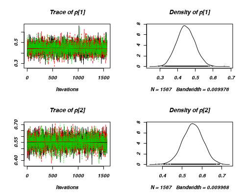
> print(plant.r2jags3)Inference for Bugs model at "../downloads/BUGSscripts/ws11.2bQ1.9.txt", fit using jags, 3 chains, each with 16667 iterations (first 1000 discarded), n.thin = 10 n.sims = 4701 iterations saved mu.vect sd.vect 2.5% 25% 50% 75% 97.5% Rhat n.eff p[1] 0.445 0.051 0.349 0.411 0.444 0.480 0.547 1.001 4700 p[2] 0.554 0.051 0.452 0.520 0.554 0.588 0.653 1.001 4700 deviance 11.817 1.935 9.948 10.456 11.219 12.628 17.103 1.001 4700 For each parameter, n.eff is a crude measure of effective sample size, and Rhat is the potential scale reduction factor (at convergence, Rhat=1). DIC info (using the rule, pD = var(deviance)/2) pD = 1.9 and DIC = 13.7 DIC is an estimate of expected predictive error (lower deviance is better). - Confirm that the MCMC sampler converged and mixed well
Show code
> library(plyr)
> library(coda)
> preds <- c("p[1]", "p[2]")
> #Trace and density plots
> plot(as.mcmc.list(alply(plant.r2jags3$BUGSoutput$sims.array[, , preds],
+     2, function(x) {
+         as.mcmc(x)
+     })))
> autocorr.diag(as.mcmc.list(alply(plant.r2jags3$BUGSoutput$sims.array[,
+     , preds], 2, function(x) {
+     as.mcmc(x)
+ })))
            p[1]     p[2]
Lag 0   1.000000  1.00000
Lag 1   0.040793  0.02910
Lag 5  -0.009471  0.01711
Lag 10  0.035296  0.01240
Lag 50  0.008957 -0.01252
> raftery.diag(as.mcmc(plant.r2jags3))
[[1]]

Quantile (q) = 0.025
Accuracy (r) = +/- 0.005
Probability (s) = 0.95

You need a sample size of at least 3746 with these values of q, r and s

[[2]]

Quantile (q) = 0.025
Accuracy (r) = +/- 0.005
Probability (s) = 0.95

You need a sample size of at least 3746 with these values of q, r and s

[[3]]

Quantile (q) = 0.025
Accuracy (r) = +/- 0.005
Probability (s) = 0.95

You need a sample size of at least 3746 with these values of q, r and s
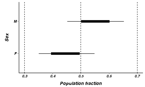
- What conclusions would you draw from the above analyses?
Comment on whether a 1:1 (0.5:0.5) or 30:70 (0.3:0.7) ratios are likely.
- How about a nice summary figure?
Show code
> preds <- c("p[1]", "p[2]")
> plant.mcmc <- as.mcmc(plant.r2jags3$BUGSoutput$sims.matrix[, preds])
> head(plant.mcmc)
Markov Chain Monte Carlo (MCMC) output:
Start = 1
End = 7
Thinning interval = 1
       p[1]   p[2]
[1,] 0.3603 0.5058
[2,] 0.4588 0.5477
[3,] 0.5483 0.5912
[4,] 0.5149 0.5482
[5,] 0.4343 0.5329
[6,] 0.4842 0.6612
[7,] 0.5680 0.5567
> plant.mcmc.sum <- adply(plant.mcmc, 2, function(x) { + data.frame(mean = mean(x), median = median(x), coda:::HPDinterval(x, p = c(0.68)), + coda:::HPDinterval(x)) + }) > plant.mcmc.sum$Sex = c("F", "M") > library(ggplot2) > p <- ggplot(plant.mcmc.sum, aes(y = mean, x = Sex)) + geom_hline(yintercept = 0.5, + linetype = "dashed") + geom_hline(yintercept = c(0.3, 0.7), linetype = "dashed") + + geom_errorbar(aes(ymin = lower.1, ymax = upper.1, x = Sex), width = 0) + + geom_errorbar(aes(ymin = lower, ymax = upper, x = Sex), width = 0, size = 3) + + scale_y_continuous("Population fraction") + geom_point() + coord_flip() + + murray_opts > p