Workshop 11.3b - Contingency tables (Bayesian)
23 April 2011
Basic χ2 references
- Logan (2010) - Chpt 16-17
- Quinn & Keough (2002) - Chpt 13-14
> library(R2jags)
> library(ggplot2)
> library(grid)
> #define my common ggplot options
> murray_opts <- opts(panel.grid.major=theme_blank(),
+ 			   panel.grid.minor=theme_blank(),
+ 			   panel.border = theme_blank(),
+ 			   panel.background = theme_blank(),
+ 			   axis.title.y=theme_text(size=15, vjust=0,angle=90),
+ 			   axis.text.y=theme_text(size=12),
+ 			   axis.title.x=theme_text(size=15, vjust=-1),
+ 			   axis.text.x=theme_text(size=12),
+ 			   axis.line = theme_segment(),
+ 			   plot.margin=unit(c(0.5,0.5,1,2),"lines")
+ )
>
> #create a convenience function for predicting from mcmc objects
> predict.mcmc <- function(mcmc, terms=NULL, mmat, trans="identity") {
+   library(plyr)
+   library(coda)
+   if(is.null(terms)) mcmc.coefs <- mcmc
+   else 	{
+      iCol<-match(terms, colnames(mcmc))
+ 	 mcmc.coefs <- mcmc[,iCol]
+   }
+   t2=")"
+   if (trans=="identity") {
+ 	t1 <- ""
+ 	t2=""
+   }else if (trans=="log") {
+ 	t1="exp("
+   }else if (trans=="log10") {
+ 	t1="10^("
+   }else if (trans=="sqrt") {
+ 	t1="("
+ 	t2=")^2"
+   }
+   eval(parse(text=paste("mcmc.sum <-adply(mcmc.coefs %*% t(mmat),2,function(x) {
+ 	data.frame(mean=",t1,"mean(x)",t2,",
+     median=",t1,"median(x)",t2,",
+ 	",t1,"coda:::HPDinterval(as.mcmc(x), p=0.68)",t2,",
+ 	",t1,"coda:::HPDinterval(as.mcmc(x))",t2,"
+     )})", sep="")))
+
+   mcmc.sum
+ }
>
>
> #create a convenience function for summarizing mcmc objects
> summary.mcmc <- function(mcmc, terms=NULL, trans="identity") {
+   library(plyr)
+   library(coda)
+   if(is.null(terms)) mcmc.coefs <- mcmc
+   else 	{
+      iCol<-grep(terms, colnames(mcmc))
+ 	 mcmc.coefs <- mcmc[,iCol]
+   }
+   t2=")"
+   if (trans=="identity") {
+ 	t1 <- ""
+ 	t2=""
+   }else if (trans=="log") {
+ 	t1="exp("
+   }else if (trans=="log10") {
+ 	t1="10^("
+   }else if (trans=="sqrt") {
+ 	t1="("
+ 	t2=")^2"
+   }
+   eval(parse(text=paste("mcmc.sum <-adply(mcmc.coefs,2,function(x) {
+ 	data.frame(mean=",t1,"mean(x)",t2,",
+     median=",t1,"median(x)",t2,",
+ 	",t1,"coda:::HPDinterval(as.mcmc(x), p=0.68)",t2,",
+ 	",t1,"coda:::HPDinterval(as.mcmc(x))",t2,"
+     )})", sep="")))
+
+   mcmc.sum$Perc <-100*mcmc.sum$median/sum(mcmc.sum$median)
+   mcmc.sum
+ }
Contingency tables
Here is a modified example from Quinn and Keough (2002). Following fire, French and Westoby (1996) cross-classified plant species by two variables: whether they regenerated by seed only or vegetatively and whether they were dispersed by ant or vertebrate vector. The two variables could not be distinguished as response or predictor since regeneration mechanisms could just as conceivably affect dispersal mode as vice versa.
Download French data set| Format of french.csv data files | ||||||||||||||||||||||||||||||||||
|---|---|---|---|---|---|---|---|---|---|---|---|---|---|---|---|---|---|---|---|---|---|---|---|---|---|---|---|---|---|---|---|---|---|---|
|
 |
|||||||||||||||||||||||||||||||||
Open the french data file. HINT.
> french <- read.table("../downloads/data/french.csv", header = T,
+     sep = ",", strip.white = T)
> head(french)
  regen disp count
1  seed  ant    25
2  seed vert     6
3   veg  ant    36
4   veg vert    21
- Fit the appropriate JAGS model
Show code
> modelString="
+ model
+ {
+   for (i in 1:n) {
+ 	count[i] ~ dpois(lambda[i])
+ 	lambda[i] <- exp(alpha+beta.disp[disp[i]]+beta.regen[regen[i]]+beta.int[disp[i],regen[i]])
+ 	y.err[i] <- count[i]-lambda[i]
+   }
+ 	alpha~dnorm(0,1.0E-6)
+ 	beta.disp[1]<-0
+ 	beta.int[1,1]<-0
+ 	for (i in 2:nDisp) {
+ 	  beta.disp[i] ~ dnorm(0,1.0E-6)
+ 	  beta.int[i,1] <- 0
+ 	}
+     beta.regen[1]<-0
+ 	for (i in 2:nRegen) {
+ 	  beta.regen[i] ~ dnorm(0,1.0E-6)
+ 	  beta.int[1,i] <- 0
+ 	}
+ 	for (i in 2:nDisp) {
+ 	  for (j in 2:nRegen) {
+ 		beta.int[i,j] ~ dnorm(0,1.0E-6)
+ 	  }
+ 	}
+   odds_vert <- lambda[4]/lambda[2]
+   odds_ant <- lambda[3]/lambda[1]
+   odds_ratio <- odds_vert/odds_ant
+
+   p1 <- step(odds_ratio-1)
+   p2 <- step(odds_ratio-1.5)
+   p3 <- step(odds_ratio-2)
+
+   #finite population standard deviations
+   sd.Resid <- sd(y.err)
+   sd.Int <- sd(beta.int)
+ }
+ "
> ## write the model to a text file (I suggest you alter the path to somewhere more relevant
> ## to your system!)
> writeLines(modelString,con="../downloads/BUGSscripts/ws11.3bQ1.1.txt")
>
> french.list <- with(french,
+ 			 list(count=count,
+ 			 disp=as.numeric(disp),
+ 			 regen=as.numeric(regen),
+ 			 nDisp=length(unique(disp)),
+ 			 nRegen=length(unique(regen)),
+ 			 n=nrow(french))
+ )
>
>
> params <- c("alpha","beta.disp","beta.regen","beta.int","odds_vert","odds_ant",
+             "odds_ratio","p1","p2","p3", "sd.Resid","sd.Int","y.err","lambda", "count")
> adaptSteps = 1000
> burnInSteps = 2000
> nChains = 3
> numSavedSteps = 50000
> thinSteps = 1
> nIter = ceiling((numSavedSteps * thinSteps)/nChains)
>
> french.r2jags <- jags(data=french.list,
+ 	  inits=NULL,#list(inits,inits,inits), #or inits=list(inits,inits,inits) # since there are three chains
+ 	  parameters.to.save=params,
+ 	  model.file="../downloads/BUGSscripts/ws11.3bQ1.1.txt",
+ 	  n.chains=3,
+ 	  n.iter=nIter,
+ 	  n.burnin=burnInSteps,
+       n.thin=10
+ 	  )
Compiling model graph Resolving undeclared variables Allocating nodes Graph Size: 54 Initializing model
> print(french.r2jags)Inference for Bugs model at "../downloads/BUGSscripts/ws11.3bQ1.1.txt", fit using jags, 3 chains, each with 16667 iterations (first 2000 discarded), n.thin = 10 n.sims = 4401 iterations saved mu.vect sd.vect 2.5% 25% 50% 75% 97.5% Rhat n.eff alpha 3.201 0.205 2.792 3.064 3.208 3.344 3.574 1.001 4100 beta.disp[1] 0.000 0.000 0.000 0.000 0.000 0.000 0.000 1.000 1 beta.disp[2] -1.508 0.473 -2.498 -1.808 -1.485 -1.182 -0.637 1.001 4400 beta.int[1,1] 0.000 0.000 0.000 0.000 0.000 0.000 0.000 1.000 1 beta.int[2,1] 0.000 0.000 0.000 0.000 0.000 0.000 0.000 1.000 1 beta.int[1,2] 0.000 0.000 0.000 0.000 0.000 0.000 0.000 1.000 1 beta.int[2,2] 0.957 0.541 -0.080 0.587 0.947 1.315 2.081 1.002 1800 beta.regen[1] 0.000 0.000 0.000 0.000 0.000 0.000 0.000 1.000 1 beta.regen[2] 0.368 0.261 -0.123 0.188 0.366 0.541 0.894 1.001 3600 count[1] 25.000 0.000 25.000 25.000 25.000 25.000 25.000 1.000 1 count[2] 6.000 0.000 6.000 6.000 6.000 6.000 6.000 1.000 1 count[3] 36.000 0.000 36.000 36.000 36.000 36.000 36.000 1.000 1 count[4] 21.000 0.000 21.000 21.000 21.000 21.000 21.000 1.000 1 lambda[1] 25.065 5.082 16.306 21.412 24.726 28.337 35.669 1.001 4400 lambda[2] 5.925 2.429 2.142 4.154 5.546 7.322 11.505 1.001 2700 lambda[3] 35.979 6.012 25.418 31.643 35.636 39.865 48.454 1.001 3500 lambda[4] 20.959 4.562 12.976 17.613 20.657 23.945 30.569 1.002 2100 odds_ant 1.495 0.402 0.884 1.207 1.442 1.717 2.446 1.001 3600 odds_ratio 3.025 1.818 0.923 1.799 2.579 3.724 8.012 1.002 1800 odds_vert 4.231 2.246 1.575 2.700 3.680 5.092 10.237 1.002 1300 p1 0.964 0.186 0.000 1.000 1.000 1.000 1.000 1.003 4100 p2 0.848 0.359 0.000 1.000 1.000 1.000 1.000 1.003 1000 p3 0.682 0.466 0.000 0.000 1.000 1.000 1.000 1.003 910 sd.Int 0.420 0.225 0.033 0.255 0.410 0.569 0.901 1.005 1000 sd.Resid 3.715 1.647 1.036 2.500 3.519 4.738 7.445 1.001 2500 y.err[1] -0.065 5.082 -10.669 -3.337 0.274 3.588 8.694 1.001 4400 y.err[2] 0.075 2.429 -5.505 -1.322 0.454 1.846 3.858 1.002 1800 y.err[3] 0.021 6.012 -12.454 -3.865 0.364 4.357 10.582 1.001 4200 y.err[4] 0.041 4.562 -9.569 -2.945 0.343 3.387 8.024 1.002 2300 deviance 23.125 3.079 19.547 21.042 22.452 24.507 30.283 1.001 4400 For each parameter, n.eff is a crude measure of effective sample size, and Rhat is the potential scale reduction factor (at convergence, Rhat=1). DIC info (using the rule, pD = var(deviance)/2) pD = 4.7 and DIC = 27.9 DIC is an estimate of expected predictive error (lower deviance is better).Show code> modelString=" + data { + N <- sum(count[1:nCell]) #Total number of species + nCell <- nDisp*nRegen + } + model + { + #Likelihood + count[1:4] ~ dmulti(p[], N) # numbers drawn from a multinomial distribution + for (i in 1:(nDisp*nRegen)) { # for each of the 4 cells in the contingency table + # calculate relative frequency of species + log(expected[i]) <- beta.disp[disp[i]] + beta.regen[regen[i]] + beta.int[disp[i], regen[i]] + y.err[i]<-log(count[i])-expected[i] + } + + total <- sum(expected[1:nCell]) # sum of the expected values + + for (i in 1:nCell) # for each of the 4 cells in the table + { + p[i] <- expected[i] / total # re-scale so expected[] are probabilities + } + + beta.disp[1] <- 0 # parameters for reference classes set to zero + for (i in 2:nDisp) { + beta.disp[i] ~ dnorm(0, 1.0E-6) # dispersal effect + beta.int[i,1]<-0 + } + beta.regen[1] <- 0 + for (i in 2:nRegen) { + beta.regen[i] ~ dnorm(0, 1.0E-6) # regeneration effect + beta.int[1,i] <- 0 + } + beta.int[1,1] <- 0 + for (i in 2:nDisp) { + for (j in 2:nRegen) { + beta.int[i,j] ~ dnorm(0, 1.0E-6) # interaction effect + } + } + + #Derivatives + odds_vert <- p[4] / p[2] # odds for vertebrate-dispersed species + odds_ant <- p[3] / p[1] # odds for ant-dispersed species + odds_ratio <- odds_vert / odds_ant # odds ratio + + p1 <- step(odds_ratio-1) + p2 <- step(odds_ratio-1.5) + p3 <- step(odds_ratio-2) + + #finite population standard deviations + sd.Resid <- sd(y.err) + sd.Int <- sd(beta.int) + } + + " > ## write the model to a text file (I suggest you alter the path to somewhere more relevant > ## to your system!) > writeLines(modelString,con="../downloads/BUGSscripts/ws11.3bQ1.1a.txt") > > french.list <- with(french, + list(f=count, + Dispersal=c(1,1,2,2), + Regeneration=c(1,2,1,2)) + ) > #french.list<-list(count=c(25, 6, 36, 21), Dispersal=c(1,1,2,2), Regeneration=c(1,2,1,2)) > > french.list <- with(french, + list(count=count, + disp=as.numeric(disp), + regen=as.numeric(regen), + nDisp=length(unique(disp)), + nRegen=length(unique(regen))) + ) > params <- c("beta.disp","beta.regen","beta.int","odds_vert","odds_ant","odds_ratio", + "total","expected","p1","p2","p3","sd.Resid","sd.Int","y.err") > adaptSteps = 1000 > burnInSteps = 2000 > nChains = 3 > numSavedSteps = 50000 > thinSteps = 1 > nIter = ceiling((numSavedSteps * thinSteps)/nChains) > > french.r2jags <- jags(data=french.list, + inits=NULL,#list(inits,inits,inits), #or inits=list(inits,inits,inits) # since there are three chains + parameters.to.save=params, + model.file="../downloads/BUGSscripts/ws11.3bQ1.1a.txt", + n.chains=3, + n.iter=nIter, + n.burnin=burnInSteps, + n.thin=10 + )Compiling data graph Resolving undeclared variables Allocating nodes Initializing Reading data back into data table Compiling model graph Resolving undeclared variables Allocating nodes Graph Size: 66 Initializing model
> print(french.r2jags)Inference for Bugs model at "../downloads/BUGSscripts/ws11.3bQ1.1a.txt", fit using jags, 3 chains, each with 16667 iterations (first 2000 discarded), n.thin = 10 n.sims = 4401 iterations saved mu.vect sd.vect 2.5% 25% 50% 75% 97.5% Rhat n.eff beta.disp[1] 0.000 0.000 0.000 0.000 0.000 0.000 0.000 1.000 1 beta.disp[2] -1.493 0.478 -2.501 -1.809 -1.475 -1.156 -0.622 1.002 1300 beta.int[1,1] 0.000 0.000 0.000 0.000 0.000 0.000 0.000 1.000 1 beta.int[2,1] 0.000 0.000 0.000 0.000 0.000 0.000 0.000 1.000 1 beta.int[1,2] 0.000 0.000 0.000 0.000 0.000 0.000 0.000 1.000 1 beta.int[2,2] 0.948 0.545 -0.067 0.572 0.933 1.319 2.025 1.002 1200 beta.regen[1] 0.000 0.000 0.000 0.000 0.000 0.000 0.000 1.000 1 beta.regen[2] 0.365 0.265 -0.151 0.187 0.361 0.546 0.882 1.003 960 expected[1] 1.000 0.000 1.000 1.000 1.000 1.000 1.000 1.000 1 expected[2] 0.250 0.117 0.082 0.164 0.229 0.315 0.537 1.002 1300 expected[3] 1.493 0.405 0.860 1.205 1.435 1.726 2.416 1.003 960 expected[4] 0.875 0.271 0.458 0.679 0.834 1.028 1.527 1.001 4400 odds_ant 1.493 0.405 0.860 1.205 1.435 1.726 2.416 1.003 960 odds_ratio 3.011 1.882 0.936 1.772 2.541 3.739 7.579 1.002 1200 odds_vert 4.203 2.347 1.565 2.647 3.638 5.100 10.106 1.002 2200 p1 0.964 0.187 0.000 1.000 1.000 1.000 1.000 1.007 1900 p2 0.843 0.364 0.000 1.000 1.000 1.000 1.000 1.001 4400 p3 0.664 0.472 0.000 0.000 1.000 1.000 1.000 1.002 2000 sd.Int 0.416 0.226 0.033 0.248 0.404 0.571 0.877 1.002 1900 sd.Resid 0.325 0.070 0.214 0.277 0.317 0.364 0.474 1.001 4400 total 3.618 0.649 2.605 3.151 3.537 3.999 5.096 1.002 1200 y.err[1] 2.219 0.000 2.219 2.219 2.219 2.219 2.219 1.000 1 y.err[2] 1.541 0.117 1.255 1.477 1.563 1.628 1.710 1.002 1300 y.err[3] 2.091 0.405 1.168 1.858 2.149 2.378 2.724 1.003 940 y.err[4] 2.170 0.271 1.518 2.017 2.210 2.365 2.586 1.002 4400 deviance 15.824 2.504 12.986 13.995 15.165 16.951 22.080 1.001 4400 For each parameter, n.eff is a crude measure of effective sample size, and Rhat is the potential scale reduction factor (at convergence, Rhat=1). DIC info (using the rule, pD = var(deviance)/2) pD = 3.1 and DIC = 19.0 DIC is an estimate of expected predictive error (lower deviance is better).
Contingency table
Arrington et al. (2002) examined the frequency with which African, Neotropical and North American fishes have empty stomachs and found that the mean percentage of empty stomachs was around 16.2%. As part of the investigation they were interested in whether the frequency of empty stomachs was related to dietary items. The data were separated into four major trophic classifications (detritivores, omnivores, invertivores, and piscivores) and whether the fish species had greater or less than 16.2% of individuals with empty stomachs. The number of fish species in each category combination was calculated and a subset of that (just the diurnal fish) is provided.
Download Arrington data set| Format of arrington.csv data file | |||||||||||||||||||||||||||||||||||||||||
|---|---|---|---|---|---|---|---|---|---|---|---|---|---|---|---|---|---|---|---|---|---|---|---|---|---|---|---|---|---|---|---|---|---|---|---|---|---|---|---|---|---|
|

|
||||||||||||||||||||||||||||||||||||||||
> arrington <- read.table("../downloads/data/arrington.csv", header = T,
+     sep = ",", strip.white = T)
> head(arrington)
  STOMACH TROPHIC
1   <16.2     DET
2   <16.2     DET
3   <16.2     DET
4   <16.2     DET
5   <16.2     DET
6   <16.2     DET
Note the format of the data file. Rather than including a compilation of the observed counts, this data file lists the categories for each individual. This example will demonstrate how to analyse two-way contingency tables from such data files. Each row of the data set represents a separate species of fish that is then cross categorised according to whether the proportion of individuals of that species with empty stomachs was higher or lower than the overall average (16.2%) and to what trophic group they belonged.
- Fit the appropriate JAGS model
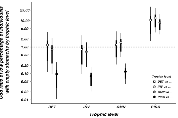
Show codeDetritivores, invertevores and omnivores are 10.4,8.6 and 12.5 times more likely to have lower percentages of individuals with empty stomachs than piscivores.
> modelString="
+ model
+ {
+   for (i in 1:n) {
+ 	freq[i] ~ dpois(lambda[i])
+ 	lambda[i] <- exp(alpha+beta.stomach[stomach[i]]+beta.trophic[trophic[i]]+beta.int[stomach[i],trophic[i]])
+ 	y.err[i] <- freq[i]-lambda[i]
+   }
+ 	alpha~dnorm(0,1.0E-6)
+ 	beta.stomach[1]<-0
+ 	beta.int[1,1]<-0
+ 	for (i in 2:nStomach) {
+ 	  beta.stomach[i] ~ dnorm(0,1.0E-6)
+ 	  beta.int[i,1] <- 0
+ 	}
+     beta.trophic[1]<-0
+ 	for (i in 2:nTrophic) {
+ 	  beta.trophic[i] ~ dnorm(0,1.0E-6)
+ 	  beta.int[1,i] <- 0
+ 	}
+ 	for (i in 2:nStomach) {
+ 	  for (j in 2:nTrophic) {
+ 		beta.int[i,j] ~ dnorm(0,1.0E-6)
+ 	  }
+ 	}
+
+
+   #odds_det <- lambda[1]/lambda[2]
+   #odds_inv <- lambda[3]/lambda[4]
+   #odds_omn <- lambda[5]/lambda[6]
+   #odds_pisc <- lambda[7]/lambda[8]
+
+   odds[1] <- lambda[1]/lambda[2]
+   odds[2] <- lambda[3]/lambda[4]
+   odds[3] <- lambda[5]/lambda[6]
+   odds[4] <- lambda[7]/lambda[8]
+
+   odds_ratio[1] <- odds[1]/odds[2]
+   odds_ratio[2] <- odds[1]/odds[3]
+   odds_ratio[3] <- odds[1]/odds[4]
+   odds_ratio[4] <- odds[2]/odds[1]
+   odds_ratio[5] <- odds[2]/odds[3]
+   odds_ratio[6] <- odds[2]/odds[4]
+   odds_ratio[7] <- odds[3]/odds[1]
+   odds_ratio[8] <- odds[3]/odds[2]
+   odds_ratio[9] <- odds[3]/odds[4]
+   odds_ratio[10] <- odds[4]/odds[1]
+   odds_ratio[11] <- odds[4]/odds[2]
+   odds_ratio[12] <- odds[4]/odds[3]
+
+ #  odds_ratio[1] <- odds_det/odds_inv
+ #  odds_ratio[2] <- odds_det/odds_omn
+ #  odds_ratio[3] <- odds_det/odds_pisc
+ #  odds_ratio[4] <- odds_inv/odds_omn
+ #  odds_ratio[5] <- odds_inv/odds_pisc
+ #  odds_ratio[6] <- odds_omn/odds_pisc
+
+   #p1 <- step(odds_ratio-1)
+   #p2 <- step(odds_ratio-1.5)
+   #p3 <- step(odds_ratio-2)
+
+   #finite population standard deviations
+   sd.Resid <- sd(lambda)
+   sd.Int <- sd(beta.int)
+ }
+ "
> ## write the model to a text file (I suggest you alter the path to somewhere more relevant
> ## to your system!)
> writeLines(modelString,con="../downloads/BUGSscripts/ws11.3bQ2.1.txt")
>
> arrington.df <- as.data.frame(table(arrington))
> arrington.list <- with(arrington.df,
+ 			 list(freq=Freq,
+ 			 stomach=as.numeric(STOMACH),
+ 			 trophic=as.numeric(TROPHIC),
+ 			 nStomach=length(unique(STOMACH)),
+ 			 nTrophic=length(unique(TROPHIC)),
+ 			 n=nrow(arrington.df))
+ )
>
> params <- c("alpha","beta.stomach","beta.trophic","beta.int",
+ 			#"odds_vert","odds_ant","odds_ratio","p1","p2","p3",
+             "sd.Resid","sd.Int","odds_ratio")
> adaptSteps = 1000
> burnInSteps = 2000
> nChains = 3
> numSavedSteps = 50000
> thinSteps = 10
> nIter = ceiling((numSavedSteps * thinSteps)/nChains)
>
> arrington.r2jags <- jags(data=arrington.list,
+ 	  inits=NULL,#list(inits,inits,inits), #or inits=list(inits,inits,inits) # since there are three chains
+ 	  parameters.to.save=params,
+ 	  model.file="../downloads/BUGSscripts/ws11.3bQ2.1.txt",
+ 	  n.chains=3,
+ 	  n.iter=nIter,
+ 	  n.burnin=burnInSteps,
+       n.thin=thinSteps
+ 	  )
Compiling model graph Resolving undeclared variables Allocating nodes Graph Size: 88 Initializing model
> print(arrington.r2jags)Inference for Bugs model at "../downloads/BUGSscripts/ws11.3bQ2.1.txt", fit using jags, 3 chains, each with 166667 iterations (first 2000 discarded), n.thin = 10 n.sims = 49401 iterations saved mu.vect sd.vect 2.5% 25% 50% 75% 97.5% Rhat n.eff alpha 2.863 0.238 2.376 2.708 2.870 3.028 3.307 1.001 49000 beta.int[1,1] 0.000 0.000 0.000 0.000 0.000 0.000 0.000 1.000 1 beta.int[2,1] 0.000 0.000 0.000 0.000 0.000 0.000 0.000 1.000 1 beta.int[1,2] 0.000 0.000 0.000 0.000 0.000 0.000 0.000 1.000 1 beta.int[2,2] 0.230 0.652 -0.974 -0.214 0.204 0.649 1.587 1.001 49000 beta.int[1,3] 0.000 0.000 0.000 0.000 0.000 0.000 0.000 1.000 1 beta.int[2,3] -0.169 0.703 -1.495 -0.648 -0.191 0.287 1.271 1.001 49000 beta.int[1,4] 0.000 0.000 0.000 0.000 0.000 0.000 0.000 1.000 1 beta.int[2,4] 2.379 0.660 1.161 1.924 2.351 2.801 3.762 1.001 49000 beta.stomach[1] 0.000 0.000 0.000 0.000 0.000 0.000 0.000 1.000 1 beta.stomach[2] -1.610 0.582 -2.860 -1.973 -1.573 -1.207 -0.566 1.001 49000 beta.trophic[1] 0.000 0.000 0.000 0.000 0.000 0.000 0.000 1.000 1 beta.trophic[2] 1.188 0.272 0.671 1.002 1.183 1.368 1.736 1.001 49000 beta.trophic[3] 0.930 0.281 0.392 0.738 0.926 1.115 1.499 1.001 49000 beta.trophic[4] -0.123 0.349 -0.813 -0.354 -0.121 0.113 0.554 1.001 49000 odds_ratio[1] 1.578 1.307 0.378 0.807 1.226 1.913 4.891 1.001 49000 odds_ratio[2] 1.094 0.975 0.224 0.523 0.826 1.332 3.564 1.001 49000 odds_ratio[3] 13.629 11.588 3.192 6.851 10.499 16.467 43.018 1.001 49000 odds_ratio[4] 0.972 0.654 0.204 0.523 0.815 1.238 2.648 1.001 49000 odds_ratio[5] 0.755 0.383 0.247 0.485 0.679 0.937 1.708 1.001 29000 odds_ratio[6] 9.408 4.311 3.787 6.397 8.532 11.414 20.087 1.001 41000 odds_ratio[7] 1.503 1.145 0.281 0.751 1.210 1.911 4.460 1.001 49000 odds_ratio[8] 1.686 0.914 0.585 1.067 1.473 2.062 4.048 1.001 29000 odds_ratio[9] 14.558 8.253 5.011 9.052 12.600 17.768 35.408 1.001 49000 odds_ratio[10] 0.114 0.077 0.023 0.061 0.095 0.146 0.313 1.001 49000 odds_ratio[11] 0.128 0.056 0.050 0.088 0.117 0.156 0.264 1.001 41000 odds_ratio[12] 0.088 0.045 0.028 0.056 0.079 0.110 0.200 1.001 49000 sd.Int 0.842 0.180 0.547 0.719 0.822 0.941 1.261 1.001 49000 sd.Resid 18.243 2.143 14.247 16.762 18.163 19.644 22.650 1.001 49000 deviance 46.166 4.142 40.277 43.194 45.510 48.375 55.804 1.001 49000 For each parameter, n.eff is a crude measure of effective sample size, and Rhat is the potential scale reduction factor (at convergence, Rhat=1). DIC info (using the rule, pD = var(deviance)/2) pD = 8.6 and DIC = 54.7 DIC is an estimate of expected predictive error (lower deviance is better).Show code> modelString=" + data { + N <- sum(freq[1:nCell]) #Total number of species + nCell <- nStomach*nTrophic + } + model + { + #Likelihood + freq[1:8] ~ dmulti(p[], N) # numbers drawn from a multinomial distribution + for (i in 1:(nStomach*nTrophic)) { # for each of the 4 cells in the contingency table + # calculate relative frequency of species + log(expected[i]) <- beta.stomach[stomach[i]] + beta.trophic[trophic[i]] + beta.int[stomach[i], trophic[i]] + y.err[i]<-log(freq[i])-expected[i] + } + + total <- sum(expected[1:nCell]) # sum of the expected values + + for (i in 1:nCell) # for each of the 4 cells in the table + { + p[i] <- expected[i] / total # re-scale so expected[] are probabilities + } + + beta.stomach[1] <- 0 # parameters for reference classes set to zero + for (i in 2:nStomach) { + beta.stomach[i] ~ dnorm(0, 1.0E-6) # dispersal effect + beta.int[i,1]<-0 + } + beta.trophic[1] <- 0 + for (i in 2:nTrophic) { + beta.trophic[i] ~ dnorm(0, 1.0E-6) # regeneration effect + beta.int[1,i] <- 0 + } + beta.int[1,1] <- 0 + for (i in 2:nStomach) { + for (j in 2:nTrophic) { + beta.int[i,j] ~ dnorm(0, 1.0E-6) # interaction effect + } + } + + #Derivatives + odds[1] <- p[1]/p[2] + odds[2] <- p[3]/p[4] + odds[3] <- p[5]/p[6] + odds[4] <- p[7]/p[8] + + odds_ratio[1] <- odds[1]/odds[2] + odds_ratio[2] <- odds[1]/odds[3] + odds_ratio[3] <- odds[1]/odds[4] + odds_ratio[4] <- odds[2]/odds[1] + odds_ratio[5] <- odds[2]/odds[3] + odds_ratio[6] <- odds[2]/odds[4] + odds_ratio[7] <- odds[3]/odds[1] + odds_ratio[8] <- odds[3]/odds[2] + odds_ratio[9] <- odds[3]/odds[4] + odds_ratio[10] <- odds[4]/odds[1] + odds_ratio[11] <- odds[4]/odds[2] + odds_ratio[12] <- odds[4]/odds[3] + + #odds_vert <- p[4] / p[2] # odds for vertebrate-dispersed species + #odds_ant <- p[3] / p[1] # odds for ant-dispersed species + #odds_ratio <- odds_vert / odds_ant # odds ratio + + p1 <- step(odds_ratio-1) + p2 <- step(odds_ratio-1.5) + p3 <- step(odds_ratio-2) + + #finite population standard deviations + sd.Resid <- sd(y.err) + sd.Int <- sd(beta.int) + } + + " > ## write the model to a text file (I suggest you alter the path to somewhere more relevant > ## to your system!) > writeLines(modelString,con="../downloads/BUGSscripts/ws11.3bQ2.1a.txt") > > arrington.df <- as.data.frame(table(arrington)) > arrington.list <- with(arrington.df, + list(freq=Freq, + stomach=as.numeric(STOMACH), + trophic=as.numeric(TROPHIC), + nStomach=length(unique(STOMACH)), + nTrophic=length(unique(TROPHIC)), + n=nrow(arrington.df)) + ) > > params <- c("beta.stomach","beta.trophic","beta.int", + #"odds_vert","odds_ant","odds_ratio","p1","p2","p3", + "sd.Resid","sd.Int","odds_ratio") > > adaptSteps = 1000 > burnInSteps = 2000 > nChains = 3 > numSavedSteps = 50000 > thinSteps = 10 > nIter = ceiling((numSavedSteps * thinSteps)/nChains) > > arrington.r2jags <- jags(data=arrington.list, + inits=NULL,#list(inits,inits,inits), #or inits=list(inits,inits,inits) # since there are three chains + parameters.to.save=params, + model.file="../downloads/BUGSscripts/ws11.3bQ2.1a.txt", + n.chains=3, + n.iter=nIter, + n.burnin=burnInSteps, + n.thin=thinSteps + )Compiling data graph Resolving undeclared variables Allocating nodes Initializing Reading data back into data table Compiling model graph Resolving undeclared variables Allocating nodes Graph Size: 118 Initializing model
> print(arrington.r2jags)Inference for Bugs model at "../downloads/BUGSscripts/ws11.3bQ2.1a.txt", fit using jags, 3 chains, each with 166667 iterations (first 2000 discarded), n.thin = 10 n.sims = 49401 iterations saved mu.vect sd.vect 2.5% 25% 50% 75% 97.5% Rhat n.eff beta.int[1,1] 0.000 0.000 0.000 0.000 0.000 0.000 0.000 1.000 1 beta.int[2,1] 0.000 0.000 0.000 0.000 0.000 0.000 0.000 1.000 1 beta.int[1,2] 0.000 0.000 0.000 0.000 0.000 0.000 0.000 1.000 1 beta.int[2,2] 0.235 0.657 -0.982 -0.212 0.204 0.657 1.606 1.001 27000 beta.int[1,3] 0.000 0.000 0.000 0.000 0.000 0.000 0.000 1.000 1 beta.int[2,3] -0.169 0.707 -1.503 -0.651 -0.186 0.291 1.270 1.001 45000 beta.int[1,4] 0.000 0.000 0.000 0.000 0.000 0.000 0.000 1.000 1 beta.int[2,4] 2.377 0.664 1.161 1.918 2.348 2.799 3.766 1.001 49000 beta.stomach[1] 0.000 0.000 0.000 0.000 0.000 0.000 0.000 1.000 1 beta.stomach[2] -1.610 0.587 -2.869 -1.976 -1.575 -1.203 -0.562 1.001 49000 beta.trophic[1] 0.000 0.000 0.000 0.000 0.000 0.000 0.000 1.000 1 beta.trophic[2] 1.187 0.274 0.664 1.000 1.181 1.368 1.741 1.001 16000 beta.trophic[3] 0.933 0.282 0.395 0.742 0.928 1.118 1.505 1.001 20000 beta.trophic[4] -0.119 0.350 -0.809 -0.351 -0.118 0.118 0.565 1.001 49000 odds_ratio[1] 1.590 1.308 0.375 0.809 1.226 1.930 4.985 1.001 27000 odds_ratio[2] 1.096 0.963 0.222 0.522 0.830 1.338 3.562 1.001 45000 odds_ratio[3] 13.628 11.641 3.192 6.809 10.460 16.425 43.217 1.001 49000 odds_ratio[4] 0.970 0.656 0.201 0.518 0.816 1.237 2.670 1.001 27000 odds_ratio[5] 0.751 0.382 0.251 0.482 0.673 0.930 1.717 1.001 49000 odds_ratio[6] 9.323 4.238 3.787 6.370 8.464 11.312 19.816 1.001 29000 odds_ratio[7] 1.509 1.156 0.281 0.747 1.205 1.917 4.496 1.001 45000 odds_ratio[8] 1.692 0.914 0.582 1.075 1.487 2.074 3.980 1.001 49000 odds_ratio[9] 14.480 8.103 4.932 9.056 12.574 17.686 34.965 1.001 49000 odds_ratio[10] 0.114 0.078 0.023 0.061 0.096 0.147 0.313 1.001 49000 odds_ratio[11] 0.128 0.056 0.050 0.088 0.118 0.157 0.264 1.001 29000 odds_ratio[12] 0.089 0.045 0.029 0.057 0.080 0.110 0.203 1.001 49000 sd.Int 0.842 0.180 0.550 0.718 0.821 0.941 1.259 1.001 49000 sd.Resid 0.512 0.241 0.254 0.346 0.438 0.608 1.146 1.001 23000 deviance 38.020 3.774 32.664 35.246 37.376 40.062 47.149 1.001 49000 For each parameter, n.eff is a crude measure of effective sample size, and Rhat is the potential scale reduction factor (at convergence, Rhat=1). DIC info (using the rule, pD = var(deviance)/2) pD = 7.1 and DIC = 45.1 DIC is an estimate of expected predictive error (lower deviance is better). - Examine the following convergence and mixing diagnostics
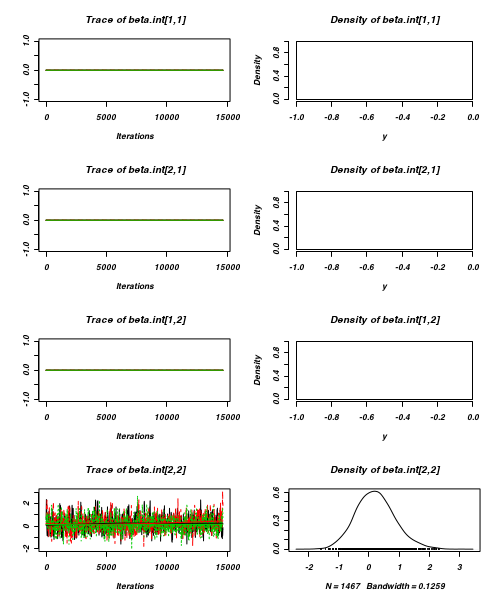
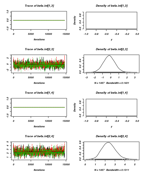
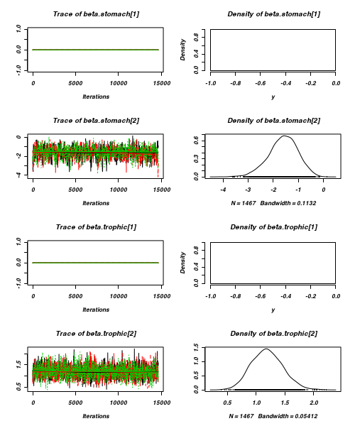
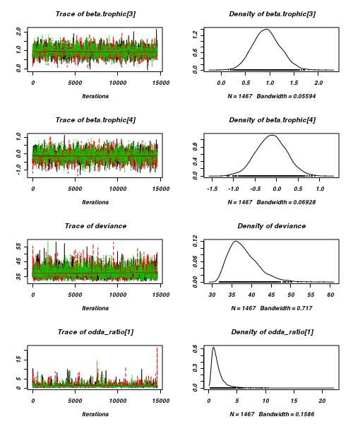
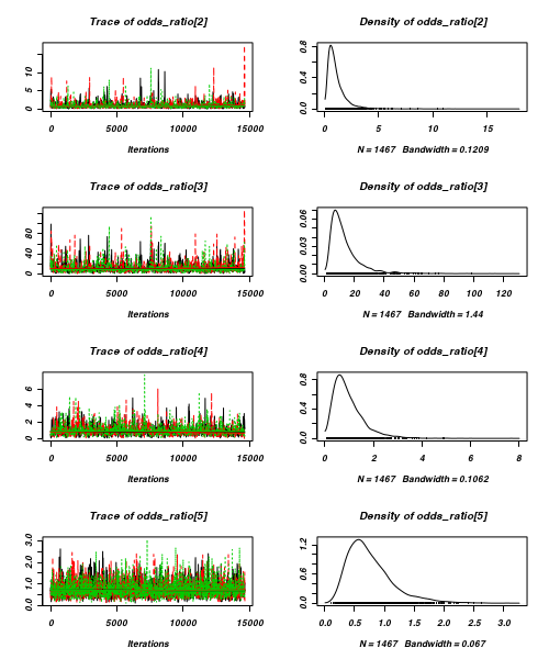
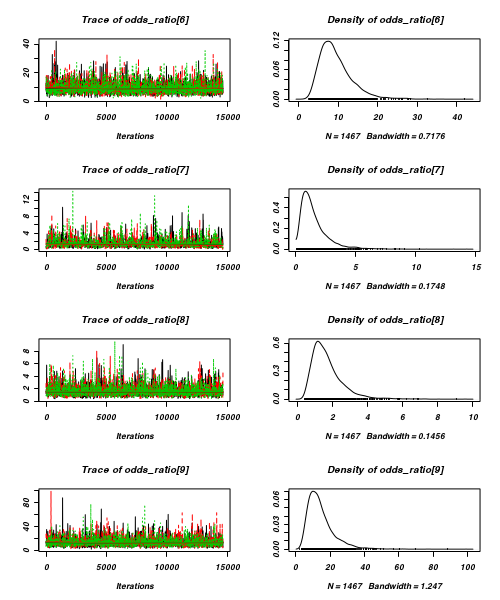
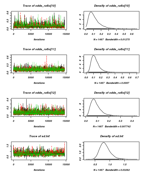
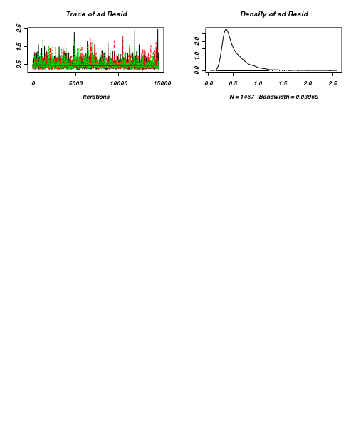
- Trace plots
View code
> plot(as.mcmc(arrington.r2jags))
- Raftery diagnostic
View code
> raftery.diag(as.mcmc(arrington.r2jags))
[[1]]

Quantile (q) = 0.025
Accuracy (r) = +/- 0.005
Probability (s) = 0.95

You need a sample size of at least 3746 with these values of q, r and s

[[2]]

Quantile (q) = 0.025
Accuracy (r) = +/- 0.005
Probability (s) = 0.95

You need a sample size of at least 3746 with these values of q, r and s

[[3]]

Quantile (q) = 0.025
Accuracy (r) = +/- 0.005
Probability (s) = 0.95

You need a sample size of at least 3746 with these values of q, r and s
- Autocorrelation
View code
> autocorr.diag(as.mcmc(arrington.r2jags))
beta.int[1,1] beta.int[2,1] beta.int[1,2] beta.int[2,2] beta.int[1,3] beta.int[2,3] Lag 0 NaN NaN NaN 1.00000 NaN 1.00000 Lag 10 NaN NaN NaN 0.57050 NaN 0.49203 Lag 50 NaN NaN NaN 0.12839 NaN 0.10125 Lag 100 NaN NaN NaN 0.01631 NaN 0.01046 Lag 500 NaN NaN NaN -0.01390 NaN -0.02106 beta.int[1,4] beta.int[2,4] beta.stomach[1] beta.stomach[2] beta.trophic[1] beta.trophic[2] Lag 0 NaN 1.000000 NaN 1.00000 NaN 1.000000 Lag 10 NaN 0.631140 NaN 0.66586 NaN 0.237851 Lag 50 NaN 0.138207 NaN 0.14940 NaN 0.054405 Lag 100 NaN 0.008053 NaN 0.01346 NaN 0.004476 Lag 500 NaN -0.031788 NaN -0.01594 NaN -0.005275 beta.trophic[3] beta.trophic[4] deviance odds_ratio[1] odds_ratio[2] odds_ratio[3] Lag 0 1.000000 1.00000 1.000000 1.0000000 1.000000 1.000000 Lag 10 0.216226 0.23222 0.065607 0.5834623 0.536551 0.619388 Lag 50 0.065008 0.02522 0.003948 0.0872946 0.061542 0.107651 Lag 100 0.015961 -0.01229 0.007765 -0.0040030 -0.001768 0.007823 Lag 500 -0.009533 -0.02130 -0.012740 0.0005963 -0.012090 -0.016683 odds_ratio[4] odds_ratio[5] odds_ratio[6] odds_ratio[7] odds_ratio[8] odds_ratio[9] Lag 0 1.00000 1.000000 1.000000 1.00000 1.000000 1.0000000 Lag 10 0.47250 -0.005009 0.012760 0.37304 -0.018679 0.0002849 Lag 50 0.12336 0.012616 0.005940 0.08626 0.015202 -0.0087040 Lag 100 0.03141 0.021019 0.003044 0.01643 0.016135 -0.0027675 Lag 500 -0.01047 -0.013556 -0.029350 -0.02650 -0.004076 -0.0241126 odds_ratio[10] odds_ratio[11] odds_ratio[12] sd.Int sd.Resid Lag 0 1.00000 1.000000 1.000000 1.000000 1.000000 Lag 10 0.55291 -0.002123 -0.002243 0.520268 0.242173 Lag 50 0.12221 0.008867 -0.010492 0.098078 0.054506 Lag 100 0.01723 -0.015839 0.003073 -0.006001 -0.001225 Lag 500 -0.03291 -0.015379 -0.032770 -0.025185 -0.012871 - How about a summary figure?
Show code
> arrington.mcmc <- as.mcmc(arrington.r2jags$BUGSoutput$sims.matrix)
> arrington.mcmc.sum <- summary(arrington.mcmc, "odds_ratio.*")
> arrington.mcmc.sum <- cbind(arrington.mcmc.sum, expand.grid(Comp1 = unique(arrington$TROPHIC),
+     Comp2 = unique(arrington$TROPHIC))[as.vector(diag(unique(arrington$TROPHIC)) ==
+     0), ])
> library(scales)
> p <- ggplot(arrington.mcmc.sum, aes(y = median, x = Comp1, group = Comp2)) +
+     geom_hline(yintercept = 1, linetype = "dashed") + geom_errorbar(aes(ymin = lower.1,
+     ymax = upper.1), stat = "identity", width = 0, position = position_dodge(0.4,
+     0)) + geom_errorbar(aes(ymin = lower, ymax = upper), stat = "identity",
+     width = 0, size = 1.5, position = position_dodge(0.4, 0)) + geom_point(aes(fill = Comp2,
+     shape = Comp2), position = position_dodge(0.4, 0), size = 3) + scale_fill_manual("Trophic level",
+     breaks = c("DET", "INV", "OMN", "PISC"), labels = c("DET vs ...", "INV vs ...",
+         "OMN vs ...", "PISC vs ..."), values = c("white", "grey90", "grey50",
+         "black")) + scale_shape_manual("Trophic level", breaks = c("DET", "INV",
+     "OMN", "PISC"), labels = c("DET vs ...", "INV vs ...", "OMN vs ...", "PISC vs ..."),
+     values = c(22, 21, 21, 21)) + scale_x_discrete("Trophic level") + scale_y_continuous("Odd ratio of low percentage of individuals\n with empty stomachs by trophic level",
+     trans = trans_new("log", "log", "exp"), breaks = function(x) as.vector(c(0.01,
+         0.1, 1, 5) %o% c(1, 2, 5))) + murray_opts + opts(legend.key = theme_blank(),
+     legend.position = c(1, 0), legend.justification = c(1, 0))
> p
Contingency tables
Here is an example (13.5) from Fowler, Cohen and Parvis (1998). A field biologist collected leaf litter from a 1 m2 quadrats randomly located on the ground at night in two locations - one was on clay soil the other on chalk soil. The number of woodlice of two different species (Oniscus and Armadilidium) were collected and it is assumed that all woodlice undertake their nocturnal activities independently. The number of woodlice are in the following contingency table.
Download Woodlice data set
Open the woodlice data file. HINT.Format of Woodlice data set WOODLICE SPECIES SOIL TYPE Oniscus Armadilidium Clay 14 6 Chalk 22 46 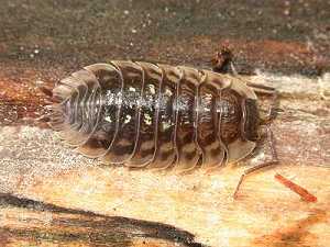 Show code
> woodlice <- read.table("../downloads/data/woodlice.csv", header = T,
+     sep = ",", strip.white = T)
> head(woodlice)
   SOIL      SPECIES COUNTS
1  Clay      oniscus     14
2  Clay armadilidium      6
3 Chalk      oniscus     22
4 Chalk armadilidium     46
- Fit the appropriate JAGS model
Show code
> modelString="
+ model
+ {
+   for (i in 1:n) {
+ 	count[i] ~ dpois(lambda[i])
+ 	lambda[i] <- exp(alpha+beta.soil[soil[i]]+beta.species[species[i]]+beta.int[soil[i],species[i]])
+ 	y.err[i] <- count[i]-lambda[i]
+   }
+ 	alpha~dnorm(0,1.0E-6)
+ 	beta.soil[1]<-0
+ 	beta.int[1,1]<-0
+ 	for (i in 2:nSoil) {
+ 	  beta.soil[i] ~ dnorm(0,1.0E-6)
+ 	  beta.int[i,1] <- 0
+ 	}
+     beta.species[1]<-0
+ 	for (i in 2:nSpecies) {
+ 	  beta.species[i] ~ dnorm(0,1.0E-6)
+ 	  beta.int[1,i] <- 0
+ 	}
+ 	for (i in 2:nSoil) {
+ 	  for (j in 2:nSpecies) {
+ 		beta.int[i,j] ~ dnorm(0,1.0E-6)
+ 	  }
+ 	}
+   odds_oniscus <- lambda[1]/lambda[3]
+   odds_armadilidium <- lambda[2]/lambda[4]
+   odds_ratio <- odds_oniscus/odds_armadilidium
+
+   p1 <- step(odds_ratio-1)
+   p2 <- step(odds_ratio-1.5)
+   p3 <- step(odds_ratio-2)
+
+   #finite population standard deviations
+   sd.Resid <- sd(y.err)
+   sd.Int <- sd(beta.int)
+ }
+ "
> ## write the model to a text file (I suggest you alter the path to somewhere more relevant
> ## to your system!)
> writeLines(modelString,con="../downloads/BUGSscripts/ws11.3bQ3.1.txt")
>
> woodlice.list <- with(woodlice,
+ 			 list(count=COUNTS,
+ 			 soil=as.numeric(SOIL),
+ 			 species=as.numeric(SPECIES),
+ 			 nSoil=length(unique(SOIL)),
+ 			 nSpecies=length(unique(SPECIES)),
+ 			 n=nrow(woodlice))
+ )
>
>
> params <- c("alpha","beta.soil","beta.species","beta.int",
+             "odds_ratio","p1","p2","p3", "sd.Resid","sd.Int","y.err","lambda", "count")
> adaptSteps = 1000
> burnInSteps = 2000
> nChains = 3
> numSavedSteps = 50000
> thinSteps = 10
> nIter = ceiling((numSavedSteps * thinSteps)/nChains)
>
> woodlice.r2jags <- jags(data=woodlice.list,
+ 	  inits=NULL,#list(inits,inits,inits), #or inits=list(inits,inits,inits) # since there are three chains
+ 	  parameters.to.save=params,
+ 	  model.file="../downloads/BUGSscripts/ws11.3bQ3.1.txt",
+ 	  n.chains=3,
+ 	  n.iter=nIter,
+ 	  n.burnin=burnInSteps,
+       n.thin=10
+ 	  )
Compiling model graph Resolving undeclared variables Allocating nodes Graph Size: 54 Initializing model
> print(woodlice.r2jags)Inference for Bugs model at "../downloads/BUGSscripts/ws11.3bQ3.1.txt", fit using jags, 3 chains, each with 166667 iterations (first 2000 discarded), n.thin = 10 n.sims = 49401 iterations saved mu.vect sd.vect 2.5% 25% 50% 75% 97.5% Rhat n.eff alpha 3.816 0.149 3.515 3.719 3.819 3.918 4.099 1.001 49000 beta.int[1,1] 0.000 0.000 0.000 0.000 0.000 0.000 0.000 1.000 1 beta.int[2,1] 0.000 0.000 0.000 0.000 0.000 0.000 0.000 1.000 1 beta.int[1,2] 0.000 0.000 0.000 0.000 0.000 0.000 0.000 1.000 1 beta.int[2,2] 1.644 0.570 0.567 1.255 1.628 2.019 2.797 1.001 49000 beta.soil[1] 0.000 0.000 0.000 0.000 0.000 0.000 0.000 1.000 1 beta.soil[2] -2.111 0.451 -3.067 -2.398 -2.085 -1.799 -1.302 1.001 49000 beta.species[1] 0.000 0.000 0.000 0.000 0.000 0.000 0.000 1.000 1 beta.species[2] -0.747 0.262 -1.269 -0.921 -0.742 -0.569 -0.245 1.001 49000 count[1] 14.000 0.000 14.000 14.000 14.000 14.000 14.000 1.000 1 count[2] 6.000 0.000 6.000 6.000 6.000 6.000 6.000 1.000 1 count[3] 22.000 0.000 22.000 22.000 22.000 22.000 22.000 1.000 1 count[4] 46.000 0.000 46.000 46.000 46.000 46.000 46.000 1.000 1 lambda[1] 13.989 3.756 7.672 11.315 13.660 16.289 22.279 1.001 49000 lambda[2] 5.992 2.445 2.205 4.215 5.662 7.417 11.675 1.001 49000 lambda[3] 22.034 4.694 13.834 18.706 21.709 25.007 32.189 1.001 49000 lambda[4] 45.935 6.779 33.600 41.242 45.571 50.305 60.274 1.001 49000 odds_ratio 6.118 4.049 1.763 3.507 5.094 7.534 16.397 1.001 49000 p1 0.999 0.031 1.000 1.000 1.000 1.000 1.000 1.009 49000 p2 0.989 0.106 1.000 1.000 1.000 1.000 1.000 1.001 49000 p3 0.957 0.202 0.000 1.000 1.000 1.000 1.000 1.001 49000 sd.Int 0.712 0.246 0.246 0.543 0.705 0.874 1.211 1.001 49000 sd.Resid 3.670 1.745 0.970 2.398 3.439 4.676 7.717 1.001 26000 y.err[1] 0.011 3.756 -8.279 -2.289 0.340 2.685 6.328 1.001 49000 y.err[2] 0.008 2.445 -5.675 -1.417 0.338 1.785 3.795 1.001 49000 y.err[3] -0.034 4.694 -10.189 -3.007 0.291 3.294 8.166 1.001 49000 y.err[4] 0.065 6.779 -14.274 -4.305 0.429 4.758 12.400 1.001 49000 deviance 22.814 2.889 19.244 20.698 22.162 24.214 30.043 1.001 49000 For each parameter, n.eff is a crude measure of effective sample size, and Rhat is the potential scale reduction factor (at convergence, Rhat=1). DIC info (using the rule, pD = var(deviance)/2) pD = 4.2 and DIC = 27.0 DIC is an estimate of expected predictive error (lower deviance is better).Show code> modelString=" + data { + nCell <- nSoil*nSpecies + N <- sum(count[1:nCell]) #Total number of woodlice + } + model + { + #Likelihood + count[1:4] ~ dmulti(p[], N) # numbers drawn from a multinomial distribution + for (i in 1:(nSoil*nSpecies)) { # for each of the 4 cells in the contingency table + # calculate relative frequency of woodlice + log(expected[i]) <- beta.soil[soil[i]] + beta.species[species[i]] + beta.int[soil[i], species[i]] + y.err[i]<-log(count[i])-expected[i] + } + + total <- sum(expected[1:nCell]) # sum of the expected values + + for (i in 1:nCell) # for each of the 4 cells in the table + { + p[i] <- expected[i] / total # re-scale so expected[] are probabilities + } + + beta.soil[1] <- 0 # parameters for reference classes set to zero + for (i in 2:nSoil) { + beta.soil[i] ~ dnorm(0, 1.0E-6) # soilersal effect + beta.int[i,1]<-0 + } + beta.species[1] <- 0 + for (i in 2:nSpecies) { + beta.species[i] ~ dnorm(0, 1.0E-6) # specieseration effect + beta.int[1,i] <- 0 + } + beta.int[1,1] <- 0 + for (i in 2:nSoil) { + for (j in 2:nSpecies) { + beta.int[i,j] ~ dnorm(0, 1.0E-6) # interaction effect + } + } + + #Derivatives + odds_oniscus <- p[1] / p[3] # odds for oniscus woodlice + odds_armadilidium <- p[2] / p[4] # odds for armadilidium woodlice + odds_ratio <- odds_oniscus / odds_armadilidium # odds ratio + + p1 <- step(odds_ratio-1) + p2 <- step(odds_ratio-1.5) + p3 <- step(odds_ratio-2) + + #finite population standard deviations + sd.Resid <- sd(y.err) + sd.Int <- sd(beta.int) + } + + " > ## write the model to a text file (I suggest you alter the path to somewhere more relevant > ## to your system!) > writeLines(modelString,con="../downloads/BUGSscripts/ws11.3bQ3.1a.txt") > > > woodlice.list <- with(woodlice, + list(count=COUNTS, + soil=as.numeric(SOIL), + species=as.numeric(SPECIES), + nSoil=length(unique(SOIL)), + nSpecies=length(unique(SPECIES))) + ) > params <- c("beta.soil","beta.species","beta.int","odds_ratio", + "total","expected","p1","p2","p3","sd.Resid","sd.Int","y.err") > adaptSteps = 1000 > burnInSteps = 2000 > nChains = 3 > numSavedSteps = 50000 > thinSteps = 10 > nIter = ceiling((numSavedSteps * thinSteps)/nChains) > > woodlice.r2jags2 <- jags(data=woodlice.list, + inits=NULL,#list(inits,inits,inits), #or inits=list(inits,inits,inits) # since there are three chains + parameters.to.save=params, + model.file="../downloads/BUGSscripts/ws11.3bQ3.1a.txt", + n.chains=3, + n.iter=nIter, + n.burnin=burnInSteps, + n.thin=thinSteps + )Compiling data graph Resolving undeclared variables Allocating nodes Initializing Reading data back into data table Compiling model graph Resolving undeclared variables Allocating nodes Graph Size: 66 Initializing model
> print(woodlice.r2jags2)Inference for Bugs model at "../downloads/BUGSscripts/ws11.3bQ3.1a.txt", fit using jags, 3 chains, each with 166667 iterations (first 2000 discarded), n.thin = 10 n.sims = 49401 iterations saved mu.vect sd.vect 2.5% 25% 50% 75% 97.5% Rhat n.eff beta.int[1,1] 0.000 0.000 0.000 0.000 0.000 0.000 0.000 1.000 1 beta.int[2,1] 0.000 0.000 0.000 0.000 0.000 0.000 0.000 1.000 1 beta.int[1,2] 0.000 0.000 0.000 0.000 0.000 0.000 0.000 1.000 1 beta.int[2,2] 1.647 0.566 0.577 1.261 1.634 2.019 2.804 1.001 49000 beta.soil[1] 0.000 0.000 0.000 0.000 0.000 0.000 0.000 1.000 1 beta.soil[2] -2.114 0.450 -3.062 -2.400 -2.091 -1.801 -1.305 1.001 49000 beta.species[1] 0.000 0.000 0.000 0.000 0.000 0.000 0.000 1.000 1 beta.species[2] -0.749 0.262 -1.274 -0.921 -0.744 -0.573 -0.247 1.001 49000 expected[1] 0.311 0.096 0.158 0.242 0.299 0.366 0.533 1.001 33000 expected[2] 0.133 0.058 0.047 0.091 0.124 0.165 0.271 1.001 49000 expected[3] 0.489 0.129 0.280 0.398 0.475 0.564 0.781 1.001 49000 expected[4] 1.000 0.000 1.000 1.000 1.000 1.000 1.000 1.000 1 odds_ratio 6.124 3.984 1.780 3.530 5.123 7.527 16.505 1.001 49000 p1 0.999 0.030 1.000 1.000 1.000 1.000 1.000 1.007 49000 p2 0.989 0.103 1.000 1.000 1.000 1.000 1.000 1.001 49000 p3 0.958 0.200 0.000 1.000 1.000 1.000 1.000 1.001 35000 sd.Int 0.713 0.245 0.250 0.546 0.707 0.874 1.214 1.001 44000 sd.Resid 0.444 0.026 0.400 0.425 0.441 0.459 0.500 1.001 49000 total 1.933 0.203 1.596 1.790 1.912 2.055 2.389 1.001 49000 y.err[1] 2.328 0.096 2.106 2.273 2.340 2.397 2.481 1.001 34000 y.err[2] 1.659 0.058 1.520 1.627 1.668 1.701 1.745 1.001 49000 y.err[3] 2.602 0.129 2.310 2.527 2.616 2.693 2.811 1.001 49000 y.err[4] 2.829 0.000 2.829 2.829 2.829 2.829 2.829 1.000 1 deviance 15.471 2.485 12.652 13.656 14.819 16.602 21.942 1.001 49000 For each parameter, n.eff is a crude measure of effective sample size, and Rhat is the potential scale reduction factor (at convergence, Rhat=1). DIC info (using the rule, pD = var(deviance)/2) pD = 3.1 and DIC = 18.6 DIC is an estimate of expected predictive error (lower deviance is better).
- Trace plots