Workshop 11.4b - Logistic regression (Bayesian)
23 April 2011
Basic χ2 references
- Logan (2010) - Chpt 16-17
- Quinn & Keough (2002) - Chpt 13-14
Logistic regression
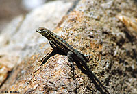
Polis et al. (1998) were intested in modelling the presence/absence of lizards (Uta sp.) against the perimeter to area ratio of 19 islands in the Gulf of California.
Download Polis data set| Format of polis.csv data file | |||||||||||||||||||||||||
|---|---|---|---|---|---|---|---|---|---|---|---|---|---|---|---|---|---|---|---|---|---|---|---|---|---|
|
|
Show code
> polis <- read.table("../downloads/data/polis.csv", header = T, sep = ",",
+     strip.white = T)
> head(polis)
      ISLAND RATIO PA
1       Bota 15.41  1
2     Cabeza  5.63  1
3    Cerraja 25.92  1
4 Coronadito 15.17  0
5     Flecha 13.04  1
6   Gemelose 18.85  0
- Fit the appropriate JAGS model
Show code
> modelString="
+ model
+ {
+   for (i in 1:n) {
+ 	pa[i] ~ dbin(p[i],1)
+ 	logit(p[i]) <- alpha+beta*ratio[i]
+   }
+ 	alpha~dnorm(0,1.0E-6)
+ 	beta ~ dnorm(0,1.0E-6)
+ }
+ "
> ## write the model to a text file (I suggest you alter the path to somewhere more relevant
> ## to your system!)
> writeLines(modelString,con="../downloads/BUGSscripts/ws11.4bQ3.1.txt")
>
> polis.list <- with(polis,
+ 			 list(pa=PA,
+ 			 ratio=RATIO,
+ 			 n=nrow(polis))
+ )
>
>
> params <- c("alpha","beta")
>
> adaptSteps = 1000
> burnInSteps = 2000
> nChains = 3
> numSavedSteps = 50000
> thinSteps = 10
> nIter = ceiling((numSavedSteps * thinSteps)/nChains)
>
> polis.r2jags <- jags(data=polis.list,
+ 	  inits=NULL,#list(inits,inits,inits), #or inits=list(inits,inits,inits) # since there are three chains
+ 	  parameters.to.save=params,
+ 	  model.file="../downloads/BUGSscripts/ws11.4bQ3.1.txt",
+ 	  n.chains=3,
+ 	  n.iter=nIter,
+ 	  n.burnin=burnInSteps,
+       n.thin=10
+ 	  )
Compiling model graph Resolving undeclared variables Allocating nodes Graph Size: 101 Initializing model
> print(polis.r2jags)Inference for Bugs model at "../downloads/BUGSscripts/ws11.4bQ3.1.txt", fit using jags, 3 chains, each with 166667 iterations (first 2000 discarded), n.thin = 10 n.sims = 49401 iterations saved mu.vect sd.vect 2.5% 25% 50% 75% 97.5% Rhat n.eff alpha 4.637 2.053 1.414 3.170 4.370 5.803 9.348 1.001 8400 beta -0.284 0.122 -0.569 -0.354 -0.268 -0.197 -0.093 1.001 8300 deviance 16.441 2.206 14.276 14.872 15.772 17.296 22.318 1.001 9500 For each parameter, n.eff is a crude measure of effective sample size, and Rhat is the potential scale reduction factor (at convergence, Rhat=1). DIC info (using the rule, pD = var(deviance)/2) pD = 2.4 and DIC = 18.9 DIC is an estimate of expected predictive error (lower deviance is better).Show codeWe could alternatively center the perimeter-area ratio predictor first. The will help with model convergence and autocorrelation.> modelString=" + model + { + for (i in 1:n) { + pa[i] ~ dbern(p[i]) + logit(p[i]) <- alpha+beta*ratio[i] + } + alpha~dnorm(0,1.0E-6) + beta ~ dnorm(0,1.0E-6) + } + " > ## write the model to a text file (I suggest you alter the path to somewhere more relevant > ## to your system!) > writeLines(modelString,con="../downloads/BUGSscripts/ws11.4bQ3.1a.txt") > > polis.list <- with(polis, + list(pa=PA, + ratio=RATIO, + n=nrow(polis)) + ) > > > params <- c("alpha","beta") > > adaptSteps = 1000 > burnInSteps = 2000 > nChains = 3 > numSavedSteps = 50000 > thinSteps = 10 > nIter = ceiling((numSavedSteps * thinSteps)/nChains) > > polis.r2jags2 <- jags(data=polis.list, + inits=NULL,#list(inits,inits,inits), #or inits=list(inits,inits,inits) # since there are three chains + parameters.to.save=params, + model.file="../downloads/BUGSscripts/ws11.4bQ3.1a.txt", + n.chains=3, + n.iter=nIter, + n.burnin=burnInSteps, + n.thin=10 + )Compiling model graph Resolving undeclared variables Allocating nodes Graph Size: 100 Initializing model
> print(polis.r2jags2)Inference for Bugs model at "../downloads/BUGSscripts/ws11.4bQ3.1a.txt", fit using jags, 3 chains, each with 166667 iterations (first 2000 discarded), n.thin = 10 n.sims = 49401 iterations saved mu.vect sd.vect 2.5% 25% 50% 75% 97.5% Rhat n.eff alpha 4.662 2.065 1.447 3.184 4.385 5.846 9.454 1.001 49000 beta -0.286 0.123 -0.570 -0.357 -0.269 -0.197 -0.094 1.001 49000 deviance 16.470 2.208 14.278 14.884 15.800 17.344 22.375 1.001 15000 For each parameter, n.eff is a crude measure of effective sample size, and Rhat is the potential scale reduction factor (at convergence, Rhat=1). DIC info (using the rule, pD = var(deviance)/2) pD = 2.4 and DIC = 18.9 DIC is an estimate of expected predictive error (lower deviance is better).Show code> modelString=" + data { + cratio <- ratio-mean(ratio) + } + model + { + for (i in 1:n) { + pa[i] ~ dbern(p[i]) + logit(p[i]) <- alpha+beta*cratio[i] + } + alpha~dnorm(0.001,1.0E-6) + beta ~ dnorm(0.001,1.0E-6) + + #Put the intercept back in the original scale + intercept <- alpha - beta*mean(ratio) + + #odds ratio + odds_ratio <- exp(beta) + + #LD50 + LD50<- (-1*intercept)/beta + } + " > ## write the model to a text file (I suggest you alter the path to somewhere more relevant > ## to your system!) > writeLines(modelString,con="../downloads/BUGSscripts/ws11.4bQ3.1b.txt") > > polis.list <- with(polis, + list(pa=PA, + ratio=RATIO, + n=nrow(polis)) + ) > > > params <- c("alpha","beta", "intercept","odds_ratio","LD50") > > adaptSteps = 1000 > burnInSteps = 2000 > nChains = 3 > numSavedSteps = 50000 > thinSteps = 10 > nIter = ceiling((numSavedSteps * thinSteps)/nChains) > > polis.r2jags3 <- jags(data=polis.list, + inits=NULL,#list(inits,inits,inits), #or inits=list(inits,inits,inits) # since there are three chains + parameters.to.save=params, + model.file="../downloads/BUGSscripts/ws11.4bQ3.1b.txt", + n.chains=3, + n.iter=nIter, + n.burnin=burnInSteps, + n.thin=10 + )Compiling data graph Resolving undeclared variables Allocating nodes Initializing Reading data back into data table Compiling model graph Resolving undeclared variables Allocating nodes Graph Size: 128 Initializing model
> print(polis.r2jags3)Inference for Bugs model at "../downloads/BUGSscripts/ws11.4bQ3.1b.txt", fit using jags, 3 chains, each with 166667 iterations (first 2000 discarded), n.thin = 10 n.sims = 49401 iterations saved mu.vect sd.vect 2.5% 25% 50% 75% 97.5% Rhat n.eff LD50 16.502 3.323 10.628 14.541 16.338 18.272 23.326 1.001 25000 alpha -0.688 0.842 -2.499 -1.208 -0.633 -0.113 0.827 1.001 19000 beta -0.284 0.122 -0.565 -0.354 -0.268 -0.197 -0.094 1.001 10000 intercept 4.640 2.041 1.439 3.184 4.363 5.802 9.400 1.001 12000 odds_ratio 0.758 0.088 0.568 0.702 0.765 0.821 0.910 1.001 10000 deviance 16.435 2.167 14.277 14.863 15.785 17.316 22.243 1.001 21000 For each parameter, n.eff is a crude measure of effective sample size, and Rhat is the potential scale reduction factor (at convergence, Rhat=1). DIC info (using the rule, pD = var(deviance)/2) pD = 2.3 and DIC = 18.8 DIC is an estimate of expected predictive error (lower deviance is better).