Workshop 11.3a - Continguency tables
23 April 2011
Basic χ2 references
- Logan (2010) - Chpt 16-17
- Quinn & Keough (2002) - Chpt 13-14
Continguency tables
Here is a modified example from Quinn and Keough (2002). Following fire, French and Westoby (1996) cross-classified plant species by two variables: whether they regenerated by seed only or vegetatively and whether they were dispersed by ant or vertebrate vector. The two variables could not be distinguished as response or predictor since regeneration mechanisms could just as conceivably affect dispersal mode as vice versa.
Download French data set| Format of french.csv data files | ||||||||||||||||||||||||||||||||||
|---|---|---|---|---|---|---|---|---|---|---|---|---|---|---|---|---|---|---|---|---|---|---|---|---|---|---|---|---|---|---|---|---|---|---|
|
 |
|||||||||||||||||||||||||||||||||
Open the french data file. HINT.
> french <- read.table("../downloads/data/french.csv", header = T,
+     sep = ",", strip.white = T)
> head(french)
  regen disp count
1  seed  ant    25
2  seed vert     6
3   veg  ant    36
4   veg vert    21
-
What null hypothesis is being tested by this test?
-
Generate a
cross table
out of the dataset in preparation for frequency analysis (HINT).
Show code> french.tab <- xtabs(count ~ regen + disp, data = french) > french.tabdisp regen ant vert seed 25 6 veg 36 21
- Fit
a 2 x 2 (two way) contingency table
(HINT), and explore the main assumption of the test by examining the expected frequencies
(HINT).
Show code
> french.x2 <- chisq.test(french.tab, correct = F)
> french.x2$exp
disp regen ant vert seed 21.49 9.511 veg 39.51 17.489
-
If the assumption is OK, test this null hypothesis and identify the following.
Show code> french.x2
	Pearson's Chi-squared test

data:  french.tab
X-squared = 2.887, df = 1, p-value = 0.08929
- X2 statistic
- df
- P value
- X2 statistic
- Calculate the odds ratio (odds of vegetative dispersal over seed dispersal for vertebrate dispersed vs ant dispersed)
Show code
> library(epitools)
> oddsratio(french.tab)
$data disp regen ant vert Total seed 25 6 31 veg 36 21 57 Total 61 27 88 $measure odds ratio with 95% C.I. regen estimate lower upper seed 1.000 NA NA veg 2.375 0.8667 7.367 $p.value two-sided regen midp.exact fisher.exact chi.square seed NA NA NA veg 0.09439 0.09832 0.08929 $correction [1] FALSE attr(,"method") [1] "median-unbiased estimate & mid-p exact CI" - What are your conclusions (statistical and biological)?
Contingency table
Arrington et al. (2002) examined the frequency with which African, Neotropical and North American fishes have empty stomachs and found that the mean percentage of empty stomachs was around 16.2%. As part of the investigation they were interested in whether the frequency of empty stomachs was related to dietary items. The data were separated into four major trophic classifications (detritivores, omnivores, invertivores, and piscivores) and whether the fish species had greater or less than 16.2% of individuals with empty stomachs. The number of fish species in each category combination was calculated and a subset of that (just the diurnal fish) is provided.
Download Arrington data set| Format of arrington.csv data file | |||||||||||||||||||||||||||||||||||||||||
|---|---|---|---|---|---|---|---|---|---|---|---|---|---|---|---|---|---|---|---|---|---|---|---|---|---|---|---|---|---|---|---|---|---|---|---|---|---|---|---|---|---|
|

|
||||||||||||||||||||||||||||||||||||||||
> arrington <- read.table("../downloads/data/arrington.csv", header = T,
+     sep = ",", strip.white = T)
> head(arrington)
  STOMACH TROPHIC
1   <16.2     DET
2   <16.2     DET
3   <16.2     DET
4   <16.2     DET
5   <16.2     DET
6   <16.2     DET
Note the format of the data file. Rather than including a compilation of the observed counts, this data file lists the categories for each individual. This example will demonstrate how to analyse two-way contingency tables from such data files. Each row of the data set represents a separate species of fish that is then cross categorised according to whether the proportion of individuals of that species with empty stomachs was higher or lower than the overall average (16.2%) and to what trophic group they belonged.
- Generate a cross table
out of the raw data file in preparation for the contingency table (HINT).
Show code
> arrington.tab <- table(arrington)
> arrington.tab
TROPHIC STOMACH DET INV OMN PISC <16.2 18 58 45 16 >16.2 4 15 8 34
- Fit the model
(HINT), test the assumptions
(HINT) and, using a
two-way contingency table,
test the null hypothesis that the percentage of empty stomachs was independent of trophic classification
(HINT).
What would you conclude form the analysis?
Show code> arrington.x2 <- chisq.test(arrington.tab) > arrington.x2$expTROPHIC STOMACH DET INV OMN PISC <16.2 15.222 50.51 36.67 34.6 >16.2 6.778 22.49 16.33 15.4
> arrington.x2
	Pearson's Chi-squared test

data:  arrington.tab
X-squared = 43.83, df = 3, p-value = 1.636e-09
-
Write the results out as though you were writing a research paper/thesis. For example (select the phrase that applies and fill in gaps with your results):
The percentage of empty stomachs was (choose the correct option)
trophic classification. (X2 =
, df =
, P =
).
-
Generate the residuals
(HINT) associated with the above contingency test and complete the following table of standardized residuals.
Show code> arrington.x2$res
       TROPHIC
STOMACH    DET    INV    OMN   PISC
  <16.2  0.712  1.054  1.375 -3.162
  >16.2 -1.067 -1.579 -2.061  4.738
< 16.2% > 16.2% DET OMN INV PISC - Calculate the odds ratios for the different trophic levels
Show code
> library(biology)
> or <- NULL
> nms <- colnames(arrington.tab)
> for (i in 1:ncol(arrington.tab)) {
+     for (j in 1:ncol(arrington.tab)) {
+         if (i == j)
+             next
+         or <- rbind(or, cbind(Comp1 = nms[i], Comp2 = nms[j], oddsratios(arrington.tab[,
+             c(i, j)])))
+     }
+ }
> or$Comp2s <- as.numeric(factor(as.character(or$Comp2)))
> opar <- par(mar = c(5, 6, 1, 1))
> plot(estimate ~ Comp2s, data = or, axes = F, ann = F, type = "n",
+     log = "y", ylim = c(min(lower), max(upper)), xlim = c(0, 5))
> abline(h = 1, lty = 2)
> with(subset(or, Comp1 == "DET"), arrows(Comp2s - 0.1, lower, Comp2s -
+     0.1, upper, code = 3, length = 0.1, ang = 90))
> points(estimate ~ I(Comp2s - 0.1), data = subset(or, Comp1 == "DET"),
+     type = "p", pch = 22, bg = "white")
> with(subset(or, Comp1 == "INV"), arrows(Comp2s - 0.05, lower, Comp2s -
+     0.05, upper, code = 3, length = 0.1, ang = 90))
> points(estimate ~ I(Comp2s - 0.05), data = subset(or, Comp1 == "INV"),
+     type = "p", pch = 21, bg = "grey90")
> with(subset(or, Comp1 == "OMN"), arrows(Comp2s + 0.05, lower, Comp2s +
+     0.05, upper, code = 3, length = 0.1, ang = 90))
> points(estimate ~ I(Comp2s + 0.05), data = subset(or, Comp1 == "OMN"),
+     type = "p", pch = 21, bg = "grey50")
> with(subset(or, Comp1 == "PISC"), arrows(Comp2s + 0.1, lower, Comp2s +
+     0.1, upper, code = 3, length = 0.1, ang = 90))
> points(estimate ~ I(Comp2s + 0.1), data = subset(or, Comp1 == "PISC"),
+     type = "p", pch = 21, bg = "black")
> axis(1, at = 1:4, labels = nms)
> axis(2, las = 1)
> mtext("Trophic level", 1, line = 3, cex = 1.5)
> mtext("Odds ratio of empty stomachs by trophic level", 2, line = 3.5,
+     cex = 1.5)
> legend("topleft", legend = nms, pch = c(22, 21, 21, 21), pt.bg = c("white",
+     "grey90", "grey50", "black"), bty = "n")
> box(bty = "l")
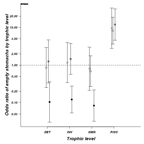
> par(opar) - What further conclusions would you draw from the standardized residuals?
Contingency tables
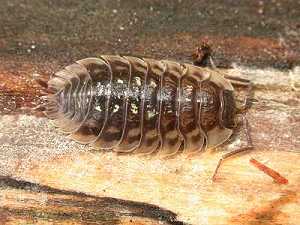
Here is an example (13.5) from Fowler, Cohen and Parvis (1998). A field biologist collected leaf litter from a 1 m2 quadrats randomly located on the ground at night in two locations - one was on clay soil the other on chalk soil. The number of woodlice of two different species (Oniscus and Armadilidium) were collected and it is assumed that all woodlice undertake their nocturnal activities independently. The number of woodlice are in the following contingency table.
Download Woodlice data set| Format of Woodlice data set | |||||||||||||
|---|---|---|---|---|---|---|---|---|---|---|---|---|---|
|
 |
||||||||||||
> woodlice <- read.table("../downloads/data/woodlice.csv", header = T,
+     sep = ",", strip.white = T)
> head(woodlice)
   SOIL      SPECIES COUNTS
1  Clay      oniscus     14
2  Clay armadilidium      6
3 Chalk      oniscus     22
4 Chalk armadilidium     46
- What null hypothesis is being tested by this test?
- Generate a
cross table
out of the dataset in preparation for frequency analysis
(HINT).
Show code> woodlice.tab <- xtabs(COUNTS ~ SOIL + SPECIES, data = woodlice) > woodlice.tabSPECIES SOIL armadilidium oniscus Chalk 46 22 Clay 6 14
- Fit
a 2 x 2 (two way) contingency table
(HINT),
and explore the main assumption of the test by examining the expected frequencies (HINT).
Show code
> woodlice.x2 <- chisq.test(woodlice.tab, correct = F)
> woodlice.x2$exp
SPECIES SOIL armadilidium oniscus Chalk 40.18 27.818 Clay 11.82 8.182
- If the assumption is OK, test this null hypothesis (HINT) and identify the following.
Show code> woodlice.x2
	Pearson's Chi-squared test

data:  woodlice.tab
X-squared = 9.061, df = 1, p-value = 0.002611
- X2 statistic
- df
- P value
- X2 statistic
-
Generate the residuals (HINT) associated with the above contingency test and complete the following table of standardized residuals.
Show code> woodlice.x2$res
       SPECIES
SOIL    armadilidium oniscus
  Chalk       0.9179 -1.1031
  Clay       -1.6924  2.0341
oniscus armadilidium CLAY CHALK - Calculate the odds ratio (of species presence) of clay vs chalk
Show code
> oddsratio(woodlice.tab)$data SPECIES SOIL armadilidium oniscus Total Chalk 46 22 68 Clay 6 14 20 Total 52 36 88 $measure odds ratio with 95% C.I. SOIL estimate lower upper Chalk 1.000 NA NA Clay 4.725 1.642 15.22 $p.value two-sided SOIL midp.exact fisher.exact chi.square Chalk NA NA NA Clay 0.003597 0.004024 0.002611 $correction [1] FALSE attr(,"method") [1] "median-unbiased estimate & mid-p exact CI"> #oniscus are 4 times more likely to have a preference for clay over chalk > # than armadilidium
- What are your conclusions (statistical and biological)?