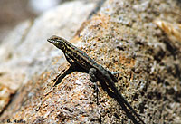
Polis et al. (1998) were intested in modelling the presence/absence of lizards (Uta sp.) against the perimeter to area ratio of 19 islands in the Gulf of California.
      ISLAND RATIO PA
1       Bota 15.41  1
2     Cabeza  5.63  1
3    Cerraja 25.92  1
4 Coronadito 15.17  0
5     Flecha 13.04  1
6   Gemelose 18.85  0
Presence absence data are clearly binary as an observation can only be in 1 of two states (1 or 0, present or absent).
Modelling the linear component (systematic) against a normal stochastic component (that is expecting the residuals to follow a normal distribution)
is clearly inappropriate. Instead, we could use a binary distribution with either a log link or probit link. For this example, we will use
the log link and thus model the residuals on the log odds scale. In a later example, we will use the probit link.
What is the null hypothesis of interest?
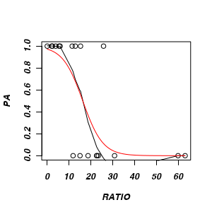
Prior to fitting the model, we need to also be sure of the structure of the systematic linear component.
For example, is the relationship linear on the log odds scale?
Show code
> plot(PA ~ RATIO, data = polis)
> with(polis, lines(lowess(PA ~ RATIO)))
>
> #check by fitting cubic spline
> library(splines)
> polis.glmS <- glm(PA ~ ns(RATIO), data = polis, family = "binomial")
> summary(polis.glmS)
Call:
glm(formula = PA ~ ns(RATIO), family = "binomial", data = polis)

Deviance Residuals:
   Min      1Q  Median      3Q     Max
-1.607  -0.638   0.237   0.433   2.099

Coefficients:
            Estimate Std. Error z value Pr(>|z|)
(Intercept)     3.56       1.68    2.12    0.034 *
ns(RATIO)     -17.24       7.89   -2.18    0.029 *
---
Signif. codes:  0 '***' 0.001 '**' 0.01 '*' 0.05 '.' 0.1 ' ' 1

(Dispersion parameter for binomial family taken to be 1)

    Null deviance: 26.287  on 18  degrees of freedom
Residual deviance: 14.221  on 17  degrees of freedom
AIC: 18.22

Number of Fisher Scoring iterations: 6
> xs <- with(polis, seq(min(RATIO), max(RATIO), l = 100))
> ys <- predict(polis.glmS, newdata = data.frame(RATIO = xs), type = "response")
> lines(xs, ys, col = "red")
>
> # The trend is more or less linear. If anything it is slightly sigmoidal
> # yet so long as it is linear within the bulk of the data, then linearity
> #   is fine.
Fitting the general linear model with a binomial error distribution (logit linkage)
(HINT).
Show code
> polis.glm <- glm(PA ~ RATIO, family = binomial, data = polis)
Assuming a probability of 0.5 for each trial, you would expect roughly 50:50 (50%) zeros and ones. So the data are not zero inflated.
As the diagnostics do not indicate any issues with the data or the fitted model, identify and interpret the following (HINT);
Show code
> polis.glm <- glm(PA ~ RATIO, family = binomial, data = polis)
> summary(polis.glm)
Call:
glm(formula = PA ~ RATIO, family = binomial, data = polis)

Deviance Residuals:
   Min      1Q  Median      3Q     Max
-1.607  -0.638   0.237   0.433   2.099

Coefficients:
            Estimate Std. Error z value Pr(>|z|)
(Intercept)    3.606      1.695    2.13    0.033 *
RATIO         -0.220      0.101   -2.18    0.029 *
---
Signif. codes:  0 '***' 0.001 '**' 0.01 '*' 0.05 '.' 0.1 ' ' 1

(Dispersion parameter for binomial family taken to be 1)

    Null deviance: 26.287  on 18  degrees of freedom
Residual deviance: 14.221  on 17  degrees of freedom
AIC: 18.22

Number of Fisher Scoring iterations: 6
sample constant (β0)
sample slope (β1)
Wald statistic (z value) for main H0
P-value for main H0
r2 value (HINT)
Show code
> 1 - (polis.glm$dev/polis.glm$null)
[1] 0.459
Another way ot test the fit of the model, and thus test the H0 that
β1 = 0, is to compare the fit of the full model to the reduce model via ANOVA.
Perform this ANOVA (HINT) and identify the following
Show code
> anova(polis.glm, test = "Chisq")
Analysis of Deviance Table

Model: binomial, link: logit

Response: PA

Terms added sequentially (first to last)


      Df Deviance Resid. Df Resid. Dev Pr(>Chi)
NULL                     18       26.3
RATIO  1     12.1        17       14.2  0.00051 ***
---
Signif. codes:  0 '***' 0.001 '**' 0.01 '*' 0.05 '.' 0.1 ' ' 1
G2 statistic
df
P value
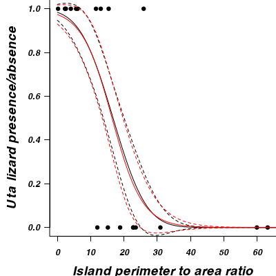
Construct a scatterplot of the presence/absence of Uta lizards against perimeter to area ratio for the 19 islands
(HINT).
Add to this plot, the predicted probability of occurances from the logistic regression (as well as 66% confidence interval - standard error).
(HINT)
Show code
> par(mar = c(4, 5, 0, 0))
> plot(PA ~ RATIO, data = polis, type = "n", ann = F, axes = F)
> points(PA ~ RATIO, data = polis, pch = 16)
> xs <- seq(0, 70, l = 1000)
> ys <- predict(polis.glm, newdata = data.frame(RATIO = xs), type = "response",
+     se = T)
> points(ys$fit ~ xs, col = "black", type = "l")
> lines(ys$fit - 1 * ys$se.fit ~ xs, col = "black", type = "l", lty = 2)
> lines(ys$fit + 1 * ys$se.fit ~ xs, col = "black", type = "l", lty = 2)
> axis(1)
> mtext("Island perimeter to area ratio", 1, cex = 1.5, line = 3)
> axis(2, las = 2)
> mtext(expression(paste(italic(Uta), " lizard presence/absence")),
+     2, cex = 1.5, line = 3)
> box(bty = "l")
Calculate the LD50 (in this case, the perimeter to area ratio with a predicted probability of 0.5) from the fitted model
(HINT).
Show code
> -polis.glm$coef[1]/polis.glm$coef[2]
(Intercept)
      16.42
Islands above this ratio are not predicted to contain lizards and islands above this ratio are expected to have lizards.
Examine the odds ratio for the occurrence of Uta lizards.
Show code
> library(biology)
> odds.ratio(polis.glm)
      Odds ratio Lower 95% CI Upper 95% CI
RATIO     0.8029       0.6593       0.9777
> #the chances of Uta lizards being present on an island declines by
> #   approximately 20% (a change factor of 0.803) for every unit increase
> #   in perimeter to area ratio.
Logistic regression - grouped binary data
Bliss (1935) examined the toxic effects of gaseous carbon disulphide on the survival of flour beetles.
He presented a number of datasets and associated analyses as a means to demonstrate models for calculating dosage curves.
In the first dataset, rather than indicating whether any individual beetle was dead or alive, Bliss (1935) recorded the number of dead and alive beetles grouped by gaseous carbon disulphide concentration.
This is another example of clearly binary data (albeit in a different form).
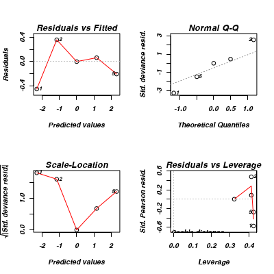
There are three obvious link function worth trying
log-link (the default)
Show code
> bliss.glm <- glm(cbind(dead, alive) ~ conc, data = bliss, family = "binomial")
> summary(bliss.glm)
Call:
glm(formula = cbind(dead, alive) ~ conc, family = "binomial",
    data = bliss)

Deviance Residuals:
      1        2        3        4        5
-0.4510   0.3597   0.0000   0.0643  -0.2045

Coefficients:
            Estimate Std. Error z value Pr(>|z|)
(Intercept)   -2.324      0.418   -5.56  2.7e-08 ***
conc           1.162      0.181    6.40  1.5e-10 ***
---
Signif. codes:  0 '***' 0.001 '**' 0.01 '*' 0.05 '.' 0.1 ' ' 1

(Dispersion parameter for binomial family taken to be 1)

    Null deviance: 64.76327  on 4  degrees of freedom
Residual deviance:  0.37875  on 3  degrees of freedom
AIC: 20.85

Number of Fisher Scoring iterations: 4
> par(mfrow = c(2, 2))
> plot(bliss.glm)
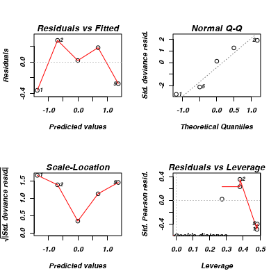
probit
Show code
> bliss.glmP <- glm(cbind(dead, alive) ~ conc, data = bliss, family = binomial(link = "probit"))
> summary(bliss.glmP)
Call:
glm(formula = cbind(dead, alive) ~ conc, family = binomial(link = "probit"),
    data = bliss)

Deviance Residuals:
      1        2        3        4        5
-0.3586   0.2749   0.0189   0.1823  -0.2754

Coefficients:
            Estimate Std. Error z value Pr(>|z|)
(Intercept)  -1.3771     0.2278   -6.05  1.5e-09 ***
conc          0.6864     0.0968    7.09  1.3e-12 ***
---
Signif. codes:  0 '***' 0.001 '**' 0.01 '*' 0.05 '.' 0.1 ' ' 1

(Dispersion parameter for binomial family taken to be 1)

    Null deviance: 64.76327  on 4  degrees of freedom
Residual deviance:  0.31367  on 3  degrees of freedom
AIC: 20.79

Number of Fisher Scoring iterations: 4
> par(mfrow = c(2, 2))
> plot(bliss.glmP)
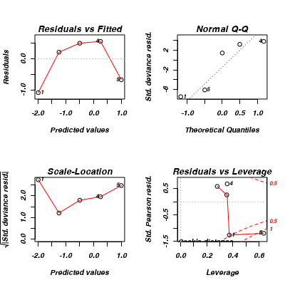
complimentary log-log
Show code
> bliss.glmC <- glm(cbind(dead, alive) ~ conc, data = bliss, family = binomial(link = "cloglog"))
> summary(bliss.glmC)
Call:
glm(formula = cbind(dead, alive) ~ conc, family = binomial(link = "cloglog"),
    data = bliss)

Deviance Residuals:
     1       2       3       4       5
-1.083   0.213   0.498   0.559  -0.672

Coefficients:
            Estimate Std. Error z value Pr(>|z|)
(Intercept)   -1.994      0.313   -6.38  1.8e-10 ***
conc           0.747      0.109    6.82  8.9e-12 ***
---
Signif. codes:  0 '***' 0.001 '**' 0.01 '*' 0.05 '.' 0.1 ' ' 1

(Dispersion parameter for binomial family taken to be 1)

    Null deviance: 64.7633  on 4  degrees of freedom
Residual deviance:  2.2305  on 3  degrees of freedom
AIC: 22.71

Number of Fisher Scoring iterations: 5
> par(mfrow = c(2, 2))
> plot(bliss.glmC)
On the basis of AIC as well as the residuals (which for the complimentary log-log model imply non-linearity),
a log link would seem appropriate.
To confirm linearity on the log odds scale
we can plot the empirical logit against concentration
Show code
> #examine linearity on the log odds scale
> # we add 1/2 (a small value) incase they are all dead or all alive.
> #This is called an empirical logit
> plot(bliss$conc, log((bliss$dead + 1/2)/(bliss$alive + 1/2)), xlab = "concentration",
+     ylab = "logit")
> abline(coef(bliss.glm), col = 2)
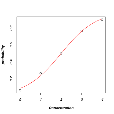
Alternatively, we could superimpose a logistic curve onto the scatterplot of proportion dead against concentration
Show code
> plot(bliss$conc, bliss$dead/(bliss$dead + bliss$alive), xlab = "Concentration",
+     ylab = "probability")
> #create an inverse logit function
> inv.logit <- function(x) exp(coef(bliss.glm)[1] + coef(bliss.glm)[2] *
+     x)/(1 + exp(coef(bliss.glm)[1] + coef(bliss.glm)[2] * x))
> #plot this function as a curve
> curve(inv.logit, add = T, col = 2)
> #seems to fit well
Given that we have elected to use the log-link model, calculate the odds-ratio
Show code
> exp(bliss.glm$coef[2])
 conc
3.196
Lets also include a summary figure
Show code
> plot(dead/(dead + alive) ~ conc, data = bliss, type = "n", ann = F,
+     axes = F)
> points(dead/(dead + alive) ~ conc, data = bliss, pch = 16)
> xs <- seq(0, 4, l = 1000)
> ys <- predict(bliss.glm, newdata = data.frame(conc = xs), type = "response",
+     se = T)
> points(ys$fit ~ xs, col = "black", type = "l")
> lines(ys$fit - 1 * ys$se.fit ~ xs, col = "black", type = "l", lty = 2)
> lines(ys$fit + 1 * ys$se.fit ~ xs, col = "black", type = "l", lty = 2)
> axis(1)
> mtext("Carbon disulphide concentration", 1, cex = 1.5, line = 3)
> axis(2, las = 2)
> mtext("Probability of death", 2, cex = 1.5, line = 3)
> box(bty = "l")
Logistic (cloglog) regression - grouped binary data
As a further demonstration of dosage curves, Bliss (1935) presented
yet another datset on the toxic effects of gaseus carbon sulphide on flour beetle mortality.
This time, Bliss (1935) documented the number of individuals exposed and dead following five hours at one of 8 dosage concentrations.
> bliss2.glmL <- glm((Mortality/Exposed) ~ Dose, data = bliss2, family = "binomial",
+     weights = Exposed)
probit - probability unit model - $\phi$ is the inverse cumulative distribution function (cdf) for the standard normal distribution
\begin{align*}
\frac{1}{\sqrt{2\pi}}\int_{-\infty}^{\alpha+\beta.X} exp\left(-\frac{1}{2}Z^2\right)dZ = \beta_0 + \beta_1Dose\\
\phi = \beta_0 + \beta_1Dose
\end{align*}
Show code
> bliss2.glmP <- glm((Mortality/Exposed) ~ Dose, data = bliss2, family = binomial(link = "probit"),
+     weights = Exposed)
> bliss2.glmC <- glm((Mortality/Exposed) ~ Dose, data = bliss2, family = binomial(link = "cloglog"),
+     weights = Exposed)
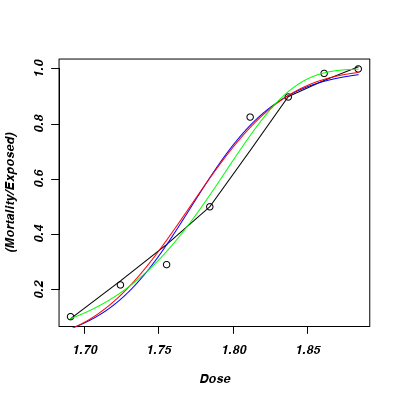
Evaluate which of the above models fits the data best on the basis of
Plotting the predicted trends
Show code
> #create the base scatterplot
> plot((Mortality/Exposed) ~ Dose, data = bliss2)
> #first plot a lowess smoother in black
> with(bliss2, lines(lowess((Mortality/Exposed) ~ Dose)))
> #create a sequence of new Dose values from which to predict mortality
> xs <- with(bliss2, seq(min(Dose), max(Dose), l = 100))
>
> # predict and plot mortality from the logit model
> ys <- predict(bliss2.glmL, newdata = data.frame(Dose = xs), type = "response")
> lines(xs, ys, col = "blue")
>
> # predict and plot mortality from the probit model
> ys <- predict(bliss2.glmP, newdata = data.frame(Dose = xs), type = "response")
> lines(xs, ys, col = "red")
>
> # predict and plot mortality from the complimentary log-log model
> ys <- predict(bliss2.glmC, newdata = data.frame(Dose = xs), type = "response")
> lines(xs, ys, col = "green")
>
> # Whilst either the log or probit models are ok (and largely
> #   indistinguishable with respect to fit), the cloglog is clearly a
> #   better fit
AIC
Show code
> #logit model
> AIC(bliss2.glmL)
[1] 15.23
> library(AICcmodavg)
> AICc(bliss2.glmL)
[1] 43.83
> #probit model
> AIC(bliss2.glmP)
[1] 14.12
> AICc(bliss2.glmP)
[1] 42.72
> #complimentary log-log model
> AIC(bliss2.glmC)
[1] 7.446
> AICc(bliss2.glmC)
[1] 36.04
> # Irrespective of whether we adopt AIC or AICc (corrected for small sample
> #   sizes), the cloglog is considered a better fit.
Which is the better link function on this occasion
Explore the parameter estimates for the cloglog model
Show code
> summary(bliss2.glmC)
Call:
glm(formula = (Mortality/Exposed) ~ Dose, family = binomial(link = "cloglog"),
    data = bliss2, weights = Exposed)

Deviance Residuals:
    Min       1Q   Median       3Q      Max
-0.8033  -0.5513   0.0309   0.3832   1.2888

Coefficients:
            Estimate Std. Error z value Pr(>|z|)
(Intercept)   -39.57       3.24   -12.2   <2e-16 ***
Dose           22.04       1.80    12.2   <2e-16 ***
---
Signif. codes:  0 '***' 0.001 '**' 0.01 '*' 0.05 '.' 0.1 ' ' 1

(Dispersion parameter for binomial family taken to be 1)

    Null deviance: 284.2024  on 7  degrees of freedom
Residual deviance:   3.4464  on 6  degrees of freedom
AIC: 33.64

Number of Fisher Scoring iterations: 4
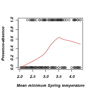
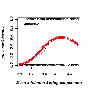
Logistic regression - polynomial
As part of a Masters thesis on the distribution and habitat suitability of the endangered Corroboree frog, Hunter (2000)
recorded the presence and absence of frogs in relation to a range of climatic factors (including mean minimum spring temperature).
> plot(pres.abs ~ meanmin, data = frogs, ylab = "Presence-absence",
+     xlab = "Mean minimum Spring temperature")
> lines(lowess(frogs$pres.abs ~ frogs$meanmin), col = 2)
> #suggests possible quadratic - optimum temperature?
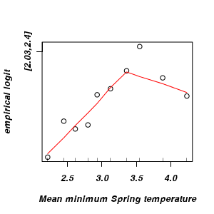
>
> #we can also look at the structure of the model by plotting on a logit
> # scale
> #after grouping the data first
> #so we need to create categories on the x-axis
> #Obviously, at the tails of a distribution, the counts diminish
> # enormously.
> #it is recomended that categories at the tails are pooled
> meanmin.cuts <- cut(frogs$meanmin, quantile(frogs$meanmin, seq(0,
+ 1, 0.1)), include.lowest = TRUE)
> yi <- tapply(frogs$pres.abs, meanmin.cuts, sum)
> #calculate the empirical logit
> emp.logit <- log((yi + 1/2)/(table(meanmin.cuts) - yi + 1/2))
> #Get the interval midpoints
> #midpt of interval (a,b) is a+(b-a)/2
> midpt <- quantile(frogs$meanmin, seq(0, 1, 0.1))[1:10] + (quantile(frogs$meanmin,
+ seq(0, 1, 0.1))[2:11] - quantile(frogs$meanmin, seq(0, 1, 0.1))[1:10])/2
>
> plot(midpt, emp.logit, xlab = "Mean minimum Spring temperature",
+ ylab = "empirical logit")
> lines(lowess(emp.logit ~ midpt), col = 2)
> rug(midpt)
>
> #fit the polynomial model
> frog.glm <- glm(pres.abs ~ meanmin + I(meanmin^2), data = frogs,
+     family = binomial)
> summary(frog.glm)
Call:
glm(formula = pres.abs ~ meanmin + I(meanmin^2), family = binomial,
    data = frogs)

Deviance Residuals:
   Min      1Q  Median      3Q     Max
-1.366  -1.003  -0.463   1.058   2.341

Coefficients:
             Estimate Std. Error z value Pr(>|z|)
(Intercept)   -21.175      5.281   -4.01  6.1e-05 ***
meanmin        11.665      3.190    3.66  0.00026 ***
I(meanmin^2)   -1.574      0.472   -3.34  0.00085 ***
---
Signif. codes:  0 '***' 0.001 '**' 0.01 '*' 0.05 '.' 0.1 ' ' 1

(Dispersion parameter for binomial family taken to be 1)

    Null deviance: 279.99  on 211  degrees of freedom
Residual deviance: 241.76  on 209  degrees of freedom
AIC: 247.8

Number of Fisher Scoring iterations: 5
> polis.glmP <- glm(PA ~ RATIO, data = polis, family = binomial(link = probit))
> summary(polis.glmP)
Call:
glm(formula = PA ~ RATIO, family = binomial(link = probit), data = polis)

Deviance Residuals:
   Min      1Q  Median      3Q     Max
-1.611  -0.677   0.188   0.415   2.055

Coefficients:
            Estimate Std. Error z value Pr(>|z|)
(Intercept)   2.1345     0.8913    2.39    0.017 *
RATIO        -0.1275     0.0522   -2.44    0.015 *
---
Signif. codes:  0 '***' 0.001 '**' 0.01 '*' 0.05 '.' 0.1 ' ' 1

(Dispersion parameter for binomial family taken to be 1)

    Null deviance: 26.287  on 18  degrees of freedom
Residual deviance: 14.164  on 17  degrees of freedom
AIC: 18.16

Number of Fisher Scoring iterations: 7
>
>
> polis.glm <- glm(PA ~ RATIO, family = binomial, data = polis)
>
>
> par(mar = c(4, 5, 0, 0))
> plot(PA ~ RATIO, data = polis, type = "n", ann = F, axes = F)
> points(PA ~ RATIO, data = polis, pch = 16)
> xs <- seq(0, 70, l = 1000)
> ys <- predict(polis.glmP, newdata = data.frame(RATIO = xs), type = "response",
+     se = T)
> points(ys$fit ~ xs, col = "black", type = "l")
> lines(ys$fit - 1 * ys$se.fit ~ xs, col = "black", type = "l", lty = 2)
> lines(ys$fit + 1 * ys$se.fit ~ xs, col = "black", type = "l", lty = 2)
>
> ys <- predict(polis.glm, newdata = data.frame(RATIO = xs), type = "response",
+     se = T)
> points(ys$fit ~ xs, col = "red", type = "l")
> lines(ys$fit - 1 * ys$se.fit ~ xs, col = "red", type = "l", lty = 2)
> lines(ys$fit + 1 * ys$se.fit ~ xs, col = "red", type = "l", lty = 2)
>
> axis(1)
> mtext("Island perimeter to area ratio", 1, cex = 1.5, line = 3)
> axis(2, las = 2)
> mtext(expression(paste(italic(Uta), " lizard presence/absence")),
+     2, cex = 1.5, line = 3)
> box(bty = "l")
>
> #the probability of Uta lizards being present declines by 0.128 (12.7
> #   units of percentage) for every 1 unit increase in perimeter to area
> #   ratio

 Show code