Jump to main navigation


Workshop 7.2a - Nested designs (mixed effects models)

25 Jan 2015

Nested ANOVA references

  • Logan (2010) - Chpt 12-14
  • Quinn & Keough (2002) - Chpt 9-11

Nested ANOVA - one between factor

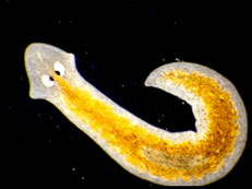
In an unusually detailed preparation for an Environmental Effects Statement for a proposed discharge of dairy wastes into the Curdies River, in western Victoria, a team of stream ecologists wanted to describe the basic patterns of variation in a stream invertebrate thought to be sensitive to nutrient enrichment. As an indicator species, they focused on a small flatworm, Dugesia, and started by sampling populations of this worm at a range of scales. They sampled in two seasons, representing different flow regimes of the river - Winter and Summer. Within each season, they sampled three randomly chosen (well, haphazardly, because sites are nearly always chosen to be close to road access) sites. A total of six sites in all were visited, 3 in each season. At each site, they sampled six stones, and counted the number of flatworms on each stone.

Download Curdies data set
Format of curdies.csv data files
SEASONSITEDUGESIAS4DUGESIA
WINTER10.6480.897
........
WINTER21.0161.004
........
WINTER30.6890.991
........
SUMMER400
........

Each row represents a different stone
SEASONSeason in which flatworms were counted - fixed factor
SITESite from where flatworms were counted - nested within SEASON (random factor)
DUGESIANumber of flatworms counted on a particular stone
S4DUGESIA4th root transformation of DUGESIA variable
Dugesia

The hierarchical nature of this design can be appreciated when we examine an illustration of the spatial and temporal scale of the measurements.

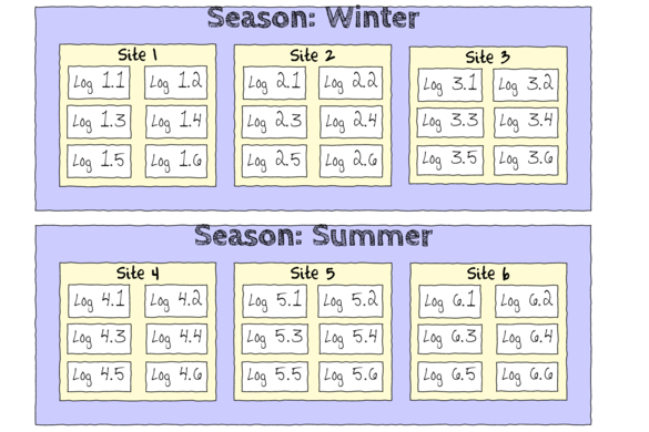
  • Within each of the two Seasons, there were three separate Sites (Sites not repeatidly measured across Seasons).
  • Within each of the Sites, six logs were selected (haphazardly) from which the number of flatworms were counted.
So the Logs (smallest sampling units) are the replicates for the Sites (six reps per Site) and the Site means are the replicates for the two Seasons (three replicates within each Season).

Open
the curdies data file.
Show code
curdies <- read.table('../downloads/data/curdies.csv', header=T, sep=',', strip.white=T)
head(curdies)
  SEASON SITE DUGESIA S4DUGES
1 WINTER    1  0.6477  0.8971
2 WINTER    1  6.0962  1.5713
3 WINTER    1  1.3106  1.0700
4 WINTER    1  1.7253  1.1461
5 WINTER    1  1.4594  1.0991
6 WINTER    1  1.0576  1.0141
  1. The SITE variable is supposed to represent a random factorial variable (which site). However, because the contents of this variable are numbers, R initially treats them as numbers, and therefore considers the variable to be numeric rather than categorical. In order to force R to treat this variable as a factor (categorical) it is necessary to first convert this numeric variable into a factor (HINT)
    .
    Show code
    curdies$SITE <- as.factor(curdies$SITE)
    

    Notice the data set - each of the nested factors is labelled differently - there can be no replicate for the random (nesting) factor.

  2. What are the main hypotheses being tested?
    1. H0 Effect 1:
    2. H0 Effect 2:
  3. In the table below, list the assumptions of nested ANOVA along with how violations of each assumption are diagnosed and/or the risks of violations are minimized.
    AssumptionDiagnostic/Risk Minimization
    I.
    II.
    III.
  4. Check these assumptions (HINT).
    Show code
    library(nlme)
    curdies.ag <- gsummary(curdies,form=~SEASON/SITE, base:::mean)
    #OR
    library(plyr)
    curdies.ag <- ddply(curdies, ~SEASON+SITE, numcolwise(mean))
    
    Note that for the effects of SEASON (Factor A in a nested model) there are only three values for each of the two season types. Therefore, boxplots are of limited value! Is there however, any evidence of violations of the assumptions (HINT)?
    Show code
    boxplot(DUGESIA~SEASON, curdies.ag)
    
    plot of chunk Q1-3a
    Show ggplot code
    library(ggplot2)
    ggplot(curdies.ag, aes(y=DUGESIA, x=SEASON)) + geom_boxplot()
    
    plot of chunk Q1-3aa
    (Y or N)
    If so, assess whether a transformation will address the violations (HINT) and then make the appropriate corrections
    Show code
    library(plyr)
    curdies.ag <- ddply(curdies, ~SEASON+SITE, function(x) {
      data.frame(S4DUGES = mean(x$DUGESIA^0.25, na.rm=TRUE))
    })
    ggplot(curdies.ag, aes(y=S4DUGES, x=SEASON)) + geom_boxplot()
    
    plot of chunk Q1-3b
  5. For each of the tests, state which error (or residual) term (state as Mean Square) will be used as the nominator and denominator to calculate the F ratio. Also include degrees of freedom associated with each term. Note this is a somewhat outdated procedure as there is far from consensus about the most appropriate estimate of denominator degrees of freedom. Nevertheless, it sometimes helps to visualize the model hierarchy this way.
    EffectNominator (Mean Sq, df)Denominator (Mean Sq, df)
    SEASON
    SITE
  6. If there is no evidence of violations, fit the model;
    S4DUGES = SEASON + SITE + CONSTANT
    using a nested ANOVA
    (HINT). Fill (HINT) out the table below, make sure that you have treated SITE as a random factor when compiling the overall results.
    Show traditional code
    curdies.aov <- aov(S4DUGES~SEASON + Error(SITE), data=curdies)
    summary(curdies.aov)
    
    Error: SITE
              Df Sum Sq Mean Sq F value Pr(>F)   
    SEASON     1   5.57    5.57    34.5 0.0042 **
    Residuals  4   0.65    0.16                  
    ---
    Signif. codes:  
    0 '***' 0.001 '**' 0.01 '*' 0.05 '.' 0.1 ' ' 1
    
    Error: Within
              Df Sum Sq Mean Sq F value Pr(>F)
    Residuals 30   4.56   0.152               
    
    summary(lm(curdies.aov))
    
    Call:
    lm(formula = curdies.aov)
    
    Residuals:
       Min     1Q Median     3Q    Max 
    -0.381 -0.262 -0.138  0.165  0.902 
    
    Coefficients: (1 not defined because of singularities)
                 Estimate Std. Error t value Pr(>|t|)
    (Intercept)    0.3811     0.1591    2.40   0.0230
    SEASONWINTER   0.7518     0.2250    3.34   0.0022
    SITE2          0.1389     0.2250    0.62   0.5416
    SITE3         -0.2651     0.2250   -1.18   0.2480
    SITE4         -0.0303     0.2250   -0.13   0.8938
    SITE5         -0.2007     0.2250   -0.89   0.3795
    SITE6              NA         NA      NA       NA
                   
    (Intercept)  * 
    SEASONWINTER **
    SITE2          
    SITE3          
    SITE4          
    SITE5          
    SITE6          
    ---
    Signif. codes:  
    0 '***' 0.001 '**' 0.01 '*' 0.05 '.' 0.1 ' ' 1
    
    Residual standard error: 0.39 on 30 degrees of freedom
    Multiple R-squared:  0.577,	Adjusted R-squared:  0.507 
    F-statistic: 8.19 on 5 and 30 DF,  p-value: 5.72e-05
    
    library(gmodels)
    ci(lm(curdies.aov))
    
                 Estimate CI lower CI upper
    (Intercept)    0.3811  0.05622   0.7060
    SEASONWINTER   0.7518  0.29235   1.2113
    SITE2          0.1389 -0.32055   0.5984
    SITE3         -0.2651 -0.72455   0.1944
    SITE4         -0.0303 -0.48978   0.4292
    SITE5         -0.2007 -0.66013   0.2588
                 Std. Error  p-value
    (Intercept)      0.1591 0.023031
    SEASONWINTER     0.2250 0.002242
    SITE2            0.2250 0.541560
    SITE3            0.2250 0.247983
    SITE4            0.2250 0.893763
    SITE5            0.2250 0.379548
    
    Show lme code
    library(nlme)
    #Fit random intercept model
    curdies.lme <- lme(S4DUGES~SEASON, random=~1|SITE, data=curdies, method='REML')
    #Fit random intercept and slope model
    curdies.lme1 <- lme(S4DUGES~SEASON, random=~SEASON|SITE, data=curdies, method='REML')
    AIC(curdies.lme, curdies.lme1)
    
                 df   AIC
    curdies.lme   4 46.43
    curdies.lme1  6 50.11
    
    anova(curdies.lme, curdies.lme1)
    
                 Model df   AIC   BIC logLik   Test L.Ratio p-value
    curdies.lme      1  4 46.43 52.54 -19.21                       
    curdies.lme1     2  6 50.11 59.27 -19.05 1 vs 2  0.3208  0.8518
    
    # Random intercepts and slope model does not fit the data better
    # Use simpler random intercepts model
    curdies.lme <- update(curdies.lme, method='REML')
    
    summary(curdies.lme)
    
    Linear mixed-effects model fit by REML
     Data: curdies 
        AIC   BIC logLik
      46.43 52.54 -19.21
    
    Random effects:
     Formula: ~1 | SITE
            (Intercept) Residual
    StdDev:     0.04009   0.3897
    
    Fixed effects: S4DUGES ~ SEASON 
                  Value Std.Error DF t-value p-value
    (Intercept)  0.3041   0.09472 30   3.211  0.0031
    SEASONWINTER 0.7868   0.13395  4   5.873  0.0042
     Correlation: 
                 (Intr)
    SEASONWINTER -0.707
    
    Standardized Within-Group Residuals:
        Min      Q1     Med      Q3     Max 
    -1.2065 -0.7681 -0.2481  0.3531  2.3209 
    
    Number of Observations: 36
    Number of Groups: 6 
    
    #Calculate the confidence interval for the effect size of the main effect of season
    intervals(curdies.lme)
    
    Approximate 95% confidence intervals
    
     Fixed effects:
                  lower   est.  upper
    (Intercept)  0.1107 0.3041 0.4976
    SEASONWINTER 0.4148 0.7868 1.1587
    attr(,"label")
    [1] "Fixed effects:"
    
     Random Effects:
      Level: SITE 
                        lower    est. upper
    sd((Intercept)) 1.875e-07 0.04009  8571
    
     Within-group standard error:
     lower   est.  upper 
    0.3026 0.3897 0.5019 
    
    #unique(confint(curdies.lme,'SEASONWINTER')[[1]])
    #Examine the ANOVA table with Type I (sequential) SS
    anova(curdies.lme)
    
                numDF denDF F-value p-value
    (Intercept)     1    30   108.5  <.0001
    SEASON          1     4    34.5  0.0042
    
    Show code - lmer
    library(lme4)
    # Fit random intercepts model
    curdies.lmer <- lmer(S4DUGES~SEASON +(1|SITE), data=curdies, REML=TRUE)
    # Fit random intercepts and slope model
    curdies.lmer1 <- lmer(S4DUGES~SEASON +(1|SITE), data=curdies, REML=TRUE)
    AIC(curdies.lmer, curdies.lmer1)
    
                  df   AIC
    curdies.lmer   4 46.43
    curdies.lmer1  4 46.43
    
    anova(curdies.lmer, curdies.lmer1)
    
    Data: curdies
    Models:
    curdies.lmer: S4DUGES ~ SEASON + (1 | SITE)
    curdies.lmer1: S4DUGES ~ SEASON + (1 | SITE)
                  Df  AIC  BIC logLik deviance Chisq Chi Df Pr(>Chisq)
    curdies.lmer   4 40.5 46.9  -16.3     32.5                        
    curdies.lmer1  4 40.5 46.9  -16.3     32.5     0      0          1
    
    summary(curdies.lmer)
    
    Linear mixed model fit by REML ['lmerMod']
    Formula: S4DUGES ~ SEASON + (1 | SITE)
       Data: curdies
    
    REML criterion at convergence: 38.4
    
    Scaled residuals: 
       Min     1Q Median     3Q    Max 
    -1.206 -0.768 -0.248  0.353  2.321 
    
    Random effects:
     Groups   Name        Variance Std.Dev.
     SITE     (Intercept) 0.00161  0.0401  
     Residual             0.15185  0.3897  
    Number of obs: 36, groups:  SITE, 6
    
    Fixed effects:
                 Estimate Std. Error t value
    (Intercept)    0.3041     0.0947    3.21
    SEASONWINTER   0.7868     0.1340    5.87
    
    Correlation of Fixed Effects:
                (Intr)
    SEASONWINTE -0.707
    
    anova(curdies.lmer)
    
    Analysis of Variance Table
           Df Sum Sq Mean Sq F value
    SEASON  1   5.24    5.24    34.5
    
    #Calculate the confidence interval for the effect size of the main effect of season
    confint(curdies.lmer)
    
                  2.5 % 97.5 %
    .sig01       0.0000 0.2279
    .sigma       0.3067 0.4882
    (Intercept)  0.1161 0.4921
    SEASONWINTER 0.5344 1.0526
    
    # Perform SAS-like p-value calculations (requires the lmerTest and pbkrtest package)
    library(lmerTest)
    curdies.lmer <- lmer(S4DUGES~SEASON +(1|SITE), data=curdies)
    summary(curdies.lmer)
    
    Linear mixed model fit by REML t-tests use Satterthwaite approximations to degrees of freedom [
    merModLmerTest]
    Formula: S4DUGES ~ SEASON + (1 | SITE)
       Data: curdies
    
    REML criterion at convergence: 38.4
    
    Scaled residuals: 
       Min     1Q Median     3Q    Max 
    -1.206 -0.768 -0.248  0.353  2.321 
    
    Random effects:
     Groups   Name        Variance Std.Dev.
     SITE     (Intercept) 0.00161  0.0401  
     Residual             0.15185  0.3897  
    Number of obs: 36, groups:  SITE, 6
    
    Fixed effects:
                 Estimate Std. Error     df t value Pr(>|t|)   
    (Intercept)    0.3041     0.0947 4.0000    3.21   0.0326 * 
    SEASONWINTER   0.7868     0.1340 4.0000    5.87   0.0042 **
    ---
    Signif. codes:  0 '***' 0.001 '**' 0.01 '*' 0.05 '.' 0.1 ' ' 1
    
    Correlation of Fixed Effects:
                (Intr)
    SEASONWINTE -0.707
    
    anova(curdies.lmer) # Satterthwaite denominator df method
    
    Analysis of Variance Table of type 3  with  Satterthwaite 
    approximation for degrees of freedom
           Sum Sq Mean Sq NumDF DenDF F.value Pr(>F)   
    SEASON   5.24    5.24     1     4    34.5 0.0042 **
    ---
    Signif. codes:  0 '***' 0.001 '**' 0.01 '*' 0.05 '.' 0.1 ' ' 1
    
    anova(curdies.lmer,ddf="Kenward-Roger") # Kenward-Roger denominator df method
    
    Analysis of Variance Table of type 3  with  Kenward-Roger 
    approximation for degrees of freedom
           Sum Sq Mean Sq NumDF DenDF F.value Pr(>F)   
    SEASON   5.24    5.24     1     4    34.5 0.0042 **
    ---
    Signif. codes:  0 '***' 0.001 '**' 0.01 '*' 0.05 '.' 0.1 ' ' 1
    
    #Examine the effect season via a likelihood ratio test
    curdies.lmer1 <- lmer(S4DUGES~SEASON +(1|SITE), data=curdies, REML=F)
    curdies.lmer2 <- lmer(S4DUGES~1 +(1|SITE), data=curdies, REML=F)
    anova(curdies.lmer1,curdies.lmer2, test="F")
    
    Data: curdies
    Models:
    ..1: S4DUGES ~ 1 + (1 | SITE)
    object: S4DUGES ~ SEASON + (1 | SITE)
           Df  AIC  BIC logLik deviance Chisq Chi Df Pr(>Chisq)    
    ..1     3 51.8 56.6  -22.9     45.8                            
    object  4 40.5 46.9  -16.3     32.5  13.3      1    0.00026 ***
    ---
    Signif. codes:  0 '***' 0.001 '**' 0.01 '*' 0.05 '.' 0.1 ' ' 1
    
  7. Check the model diagnostics
    • Residual plot
    • Show traditional code
      par(mfrow=c(2,2))
      plot(lm(curdies.aov))
      
      plot of chunk Q1-5d
      Show lme code
      plot(curdies.lme)
      
      plot of chunk Q1-5e
  8. For each of the tests, state which error (or residual) term (state as Mean Square) will be used as the nominator and denominator to calculate the F ratio. Also include degrees of freedom associated with each term.
    Source of variationdfMean SqF-ratioP-value
    SEASON
    SITE
    Residuals   

    EstimateMeanLower 95% CIUpper 95% CI
    Summer
    Effect size (Winter-Summer)

  Reading data into R

Ensure that the working directory is pointing to the path containing the file to be imported before proceeding.
To import data into R, we read the contents of a file into a data frame. The general format of the command for reading data into a data frame is

> name <- read.table('filename.csv', header=T, sep=',', row.names=column, strip.white=T)

where name is a name you wish the data frame to be referred to as, filename.csv is the name of the csv file that you created in excel and column is the number of the column that had row labels (if there were any). The argument header=T indicates that the variable (vector) names will be created from the names supplied in the first row of the file. The argument sep=',' indicates that entries in the file are separated by a comma (hence a comma delimited file). If the data file does not contain row labels, or you are not sure whether it does, it is best to omit the row.names=column argument. The strip.white=T arguement ensures that no leading or trailing spaces are left in character names (these can be particularly nasty in categorical variables!).

As an example
phasmid <- read.data('phasmid.csv', header=T, sep=',', row.names=1, strip.white=T)

End of instructions

  Nested ANOVA

A nested ANOVA is a simple extension of the single factor ANOVA. An additional factor (Factor B) is added that is nested within the main factor of interest (Factor A). Nested factors are incorporated in situations where researches envisage potentially large amounts of variation between different sets of replicates within the main Factor.
For example, a limnologist investigating the effect of flow (Factor A: high, medium and low) on macroinvertebate density, might collect samples from a number of high, medium and low flow streams. However, the limnologist might expect that many other factors (perhaps more important than stream flow) also influence the density of macroinvertebrates and that even samples collected in close proximity to one another might be expected to vary considerably in density of macroinvertebrates. Such variability increases the unexplained variability and therefore has the potential to make it very difficult to pick up the effect of the actual factor of interest (in this case flow).
In an attempt to combat this, the researcher decides to collect multiple samples from within each stream. If some of the unexplained variability can be explained by variation between samples within streams, then the test of flow will be more sensitive.
This is called a nested ANOVA, an additional factor (Factor B: stream) has been introduce within the main factor (Factor A: flow). Factor A is a fixed factor as we are only interested in the specific levels chosen (e.g. high, medium and low flow). Factor B however, is a random as we are not just interested in the specific streams that were sampled, we are interested in all the possible streams that they represent. In a nested ANOVA the categories of the Factor B nested within each level of Factor A are different. E.g. the streams used for each flow type are different. Therefore it is not possible to test for an interaction between Flow type and stream.

There are two null hypotheses being tested in a two factor nested ANOVA. H0 main effect: no effect of Factor A (flow) H0: = &mu1 = &mu2 = ... = &mui = &mu (as for single factor ANOVA). H0 nesting effect: no effect of Factor B (stream) nested within Factor A (flow). Technically it is that there is no added variance due to differences between all the possible levels of Factor B with any level of Factor A. E.g., that there is no added variance due to differences between all possible high flow streams, or between all possible medium flow streams or between all possible low flow streams. Diagram shows layout of nested design with three treatments (different pattern fills).

End of instructions

  Convert numeric variable into a factor

> data$var <- as.factor(data$var)

where data is the name of the data set and var is the name of the variable to be made into a factor. While there is no visible evidence that the data are any different, R will now treat the variable as a factor rather than as a numeric variable.

End of instructions

  Nested ANOVA assumptions

In ANOVA, the assumptions of normality and variance homogeneity apply to the residuals for the test of interest. In this example, the nested factor (Factor B, SITE) is random. Therefore, the normality and heterogeneity of variance assumptions for Factor A (SEASON) must be based on the distribution, mean and variance of the response variable (S4DUGES) for each level of Factor A using the means of Factor B within each Factor A as the observations (since the error term for Factor A (SEASON) is the variation in the response variable between categories of Factor B within each level of Factor A (MSSITE). Calculate the mean from each level of Factor B (SITE), and use these means to calculate the mean, variance and distribution of each level of Factor A (SEASON).

# aggregate the data set by calculating the means for each level of the nesting factor
> name.ag <- aggregate(dataset, list(Name1=FactorA, Name2=FactorB), mean)
#OR perhaps more efficiently
library(lme4)
name.ag <- gsummary(dataset, groups=FactorB)
# use the aggregated means to produce the boxplots
> boxplot(dv~FactorA, name.ag)

where name.ag is a name given to the new aggregated data set, dataset is the name of the original data set, Name1 and Name2 are names to appear in the aggregated data set that represent FactorA (Main within factor) and FactorB (nesting factor) respectively. Finally, dv is the name of the dependent variable.

This data set generates two boxplots, each constructed from only 3 values and thus of questionable value.

End of instructions

  Nested ANOVA assumptions

# fit the heirachical linear model
> name.aov <- aov(dv~FactorA + Error(FactorB), data=data)
# print out the ANOVA strata
> summary(name.aov)

where name.aov is a name provided to store the fitted model, dv is the dependent variable, FactorA is the main fixed factor and FactorB is the random nested factor. data is the name of the data set. The 'Error()' argument defines additional error (residual) strata, hence the above template indicates that Factor should be tested against FactorB.
For example:

# fit the heirachical linear model
> curdies.aov <- aov(S4DUGES~SEASON + Error(SITE), data=curdies)
# print out the ANOVA strata
> summary(curdies.aov)

In recognition that Factor is a random nested factor, and thus of little interest, the F-ratio is not provided. Since the effect of FactorB is tested against the overal residual (error) term, to obtain the F-ratio for the test of FactorB, fit the model without defining the an additional error strata. Note that when you do this, all terms are tested against the residual term and therefore, any fixed factors above the random factors (in the hierarchy) will be incorrectly calculated.

> curdies.aov1 <- aov(S4DUGES~SEASON + SITE, data=curdies)
> summary(curdies.aov)

End of instructions

  Two factor ANOVA

Statistical models that incorporate more than one categorical predictor variable are broadly referred to as multivariate analysis of variance. There are two main reasons for the inclusion of multiple factors:

  1. To attempt to reduce the unexplained (or residual) variation in the response variable and therefore increase the sensitivity of the main effect test.
  2. To examine the interaction between factors. That is, whether the effect of one factor on the response variable is dependent on other factor(s) (consistent across all levels of other factor(s)).

Fully factorial linear models are used when the design incorporates two or more factors (independent, categorical variables) that are crossed with each other. That is, all combinations of the factors are included in the design and every level (group) of each factor occurs in combination with every level of the other factor(s). Furthermore, each combination is replicated.

In fully factorial designs both factors are equally important (potentially), and since all factors are crossed, we can also test whether there is an interaction between the factors (does the effect of one factor depend on the level of the other factor(s)). Graphs above depict a) interaction, b) no interaction.


For example, Quinn (1988) investigated the effects of season (two levels, winter/spring and summer/autumn) and adult density (four levels, 8, 15, 30 and 45 animals per 225cm2) on the number of limpet egg masses. As the design was fully crossed (all four densities were used in each season), he was also able to test for an interaction between season and density. That is, was the effect of density consistent across both seasons and, was the effect of season consistent across all densities.

Diagram shows layout of 2 factor fully crossed design. The two factors (each with two levels) are color (black or gray) and pattern (solid or striped). There are three experimental units (replicates) per treatment combination.


End of instructions

  Two-factor ANOVA

> name.aov <- aov(dv~factor1 * factor2, data=data)

where dv is the name of the numeric vector (dependent variable), factor1 and factor2 are the names of the factors (categorical or factor variables) and data is the name of the data frame (data set).

End of instructions

  Fully factorial ANOVA assumption checking

The assumptions of normality and homogeneity of variance apply to each of the factor level combinations, since it is the replicate observations of these that are the test residuals. If the design has two factors (IV1 and IV2) with three and four levels (groups) respectively within these factors, then a boxplot of each of the 3x4=12 combinations needs to be constructed. It is recommended that a variable (called GROUP) be setup to represent the combination of the two categorical (factor) variables.

Simply construct a boxplot with the dependent variable on the y-axis and GROUP on the x-axis. Visually assess whether the data from each group is normal (or at least that the groups are not all consistently skewed in the same direction), and whether the spread of data is each group is similar (or at least not related to the mean for that group). The GROUP variable can also assist in calculating the mean and variance for each group, to further assess variance homogeneity.

End of instructions

  Factorial boxplots

> boxplot(dv~factor1*factor2,data=data)

where dv is the name of the numeric vector (dependent variable), factor1 and factor2 are the names of the factors (categorical or factor variables) and data is the name of the data frame (data set). The '~' is used in formulas to represent that the left hand side is proportional to the right hand side.

End of instructions

  Plotting mean vs variance

# first calculate the means and variances
> means <- tapply(data$dv, list(data$factor1, data$factor2), mean)
> vars <- tapply(data$dv, list(data$factor1, data$factor2), var)
# then plot the mean against variance
> plot(means,vars)

where dv is the name of the numeric vector (dependent variable), factor1 and factor2 are the names of the factors (categorical or factor variables) and data is the name of the data frame (data set).

End of instructions

  Model balance

Balanced models are those models that have equal sample sizes for each level of a treatment. Unequal sample sizes are generally problematic for statistical analyses as they can be the source of unequal variances. They are additionally problematic for multifactor designs because of the way that total variability is partitioned into the contributions of each of the main effects as well as the contributions of interactions (ie the calculations of sums of squares and degrees of freedom). Sums of squares (and degrees of freedom) are usually (type I SS) partitioned additively. That is:
SSTotal=SSA+SSB+SSAB+SSResidual, and
dfTotal=dfA+dfB+dfAB+dfResidual
. In practice, these formulas are used in reverse. For example, if the model was entered as DV~A+B+AB, first SSResidual is calculated followed by SSAB, then SSB. SSA is thus calculated as the total sums of squares minus what has already been partitioned off to other terms (SSA=SSTotal-SSB+SSAB+SSResidual). If the model is balanced, then it doesn't matter what order the model is constructed (DV~B+A+AB will be equivalent).

However, in unbalanced designs, SS cannot be partitioned additively, that is the actual SS of each of the terms does not add up to SSTotal (SSTotal=SSA+SSB+SSAB+SSResidual). Of course, when SS is partitioned it all must add up. Consequently, the SS of the last term to be calculated will not be correct. Therefore, in unbalanced designs, SS values for the terms are different (and therefore so are the F-ratios etc) depending on the order in which the terms are added - an undesirable situation.

To account for this, there are alternative methods of calculating SS for the main effects (all provide same SS for interaction terms and residuals).

It turns out that it is relatively easy to determine whether or not the model is balanced or not - use the following syntax:

> !is.list(replications(formula,data))

where formula is the model formula (for example, MASS~SITUATION*MONTH) and data is the name of data set.
If this function returns a TRUE, your model is balanced. If it returns a FALSE then your model is not balanced and you should consider using Type II or III SS methods.

End of instructions

  Linear regression diagnostics

> plot(name.lm)

where name.lm is the name of a fitted linear model. You will be prompted to hit return to cycle through a series of four diagnostic plots. The first (and most important of these) is the Residual Plot.

End of instructions

  ANOVA table

#print a summary of the ANOVA table
> anova(name.aov)

where name.aov is the name of a fitted linear model.

End of instructions

  Interaction plot

Interaction plots display the degree of consistency (or lack of) of the effect of one factor across each level of another factor. Interaction plots can be either bar or line graphs, however line graphs are more effective. The x-axis represents the levels of one factor, and a separate line in drawn for each level of the other factor. The following interaction plots represent two factors, A (with levels A1, A2, A3) and B (with levels B1, B2).


The parallel lines of first plot clearly indicate no interaction. The effect of factor A is consistent for both levels of factor B and visa versa. The middle plot demonstrates a moderate interaction and bottom plot illustrates a severe interaction. Clearly, whether or not there is an effect of factor B (e.g. B1 > B2 or B2 > B1) depends on the level of factor A. The trend is not consistent.

End of instructions

  R Interaction plot

> interaction.plot(dataset$Factor1, dataset$Factor2, dataset$dv)

where Factor1 is the name of the categical variable (factor) with the most levels (this will be used for the x-axis), Factor2 is the name of the other factorial variable (this will be used to produce the different lines) and dv is the name of the dependent variable within the dataset data set
For example:

> interaction.plot(copper$DIST, copper$COPPER, dataset$WORMS)

End of instructions

  Specific comparisons of means

Following a significant ANOVA result, it is often desirable to specifically compare group means to determine which groups are significantly different. However, multiple comparisons lead to two statistical problems. Firstly, multiple significance tests increase the Type I errors (&alpha, the probability of falsely rejecting H0). E.g., testing for differences between 5 groups requires ten pairwise comparisons. If the &alpha for each test is 0.05 (5%), then the probability of at least one Type I error for the family of 10 tests is 0.4 (40%). Secondly, the outcome of each test needs to be independent (orthogonality). E.g. if A>B and B>C then we already know the result of A vs. C.

Post-hoc unplanned pairwise comparisons (e.g. Tukey's test) compare all possible pairs of group means and are useful in an exploratory fashion to reveal major differences. Tukey's test control the family-wise Type I error rate to no more that 0.05. However, this reduces the power of each of the pairwise comparisons, and only very large differences are detected (a consequence that exacerbates with an increasing number of groups).

Planned comparisons are specific comparisons that are usually planned during the design stage of the experiment. No more than (p-1, where p is the number of groups) comparisons can be made, however, each comparison (provided it is non-orthogonal) can be tested at &alpha = 0.05. Amongst all possible pairwise comparisons, specific comparisons are selected, while other meaningless (within the biological context of the investigation) are ignored.

Planned comparisons are defined using what are known as contrasts coefficients. These coefficients are a set of numbers that indicate which groups are to be compared, and what the relative contribution of each group is to the comparison. For example, if a factor has four groups (A, B, C and D) and you wish to specifically compare groups A and B, the contrast coefficients for this comparison would be 1, -1, 0,and 0 respectively. This indicates that groups A and B are to be compared (since their signs oppose) and that groups C and D are omitted from the specific comparison (their values are 0).

It is also possible to compare the average of two or more groups with the average of other groups. For example, to compare the average of groups A and B with the average of group C, the contrast coefficients would be 1, 1, -2, and 0 respectively. Note that 0.5, 0.5, 1 and 0 would be equivalent.

The following points relate to the specification of contrast coefficients:

  1. The sum of the coefficients should equal 0
  2. Groups to be compared should have opposing signs

End of instructions

  Tukey's Test

# load the 'multcomp' package
> library(multcomp)
# perform Tukey's test
> summary(simtest(dv~factor1*factor2, whichf='factor', data=data, type="Tukey"))
# OR the more up to date method
> summary(glht(data.aov, linfct=mcp(factor="Tukey")))

where dv is the name of the numeric vector (dependent variable), factor1 and factor2 are the names of the factors (categorical or factor variables), and data is the name of the data frame (data set). The argument tyoe="Tukey" indicates that a Tukeys p-value adjustments should be made. When the linear model contains multiple categorical predictor variables, the arguement whichf='' must be used to indicate which factor the Tukey's test should be performed on.

The coefficients list the specific comparisons made. Each line represents a specific hypothesis test including difference between groups, t-value, raw p value and Tukey's adjusted p value (the other values presented are not important for BIO3011).

End of instructions

  Simple Main Effects

> library(biology)
> quinn.aov1 <- aov(SQRTRECRUITS~DENSITY, data=quinn, subset=c(SEASON=='Summer'))
> AnovaM(lm(quinn.aov1), lm(quinn.aov),type="II")

Subset, type in the name of the other categorical variable followed by == (two equals signs) and the name of one of the levels (surrounded by single quotation marks) of this factor. For example, if you had a categorical variable called TEMPERATURE and it consisted of three levels (High, Medium and Low), to perform a anova using only the High temperature data, the subset expression would be TEMPERATURE=='High'.

End of instructions

  Randomized complete block (RCB) designs

These are designs where one factor is a blocking variable (Factor B) and the other variable (Factor A) is the main treatment factor of interest. These designs are used in situations where the environment is potentially heterogeneous enough to substantially increase the variability in the response variable and thus obscure the effects of the main factor. Experimental units are grouped into blocks (units of space or time that are likely to have less variable background conditions) and then each level of the treatment factor is applied to a single unit within each block. By grouping the experimental units together into blocks, some of the total variability in the response variable that is not explained by the main factor may be explained by the blocks. If so, the residual (unexplained) variation will be reduced resulting in more precise estimates of parameters and more powerful tests of treatments.

A plant ecologist was investigating the effects of leaf damage on plant chemical defenses. Since individual trees vary greatly in the degree of chemical defense, she applied each of three artificial leaf damage treatments (heavy, medium and light damage) to each tree. She applied one of three treatments to three branches within eight randomly selected trees. Trees were the blocks. The diagram shows the layout of a blocking design. The main factor has three treatments (pattern fills), each of which are applied randomly within 3 randomly selected blocks. The decision to include a blocking factor (rather than single factor, completely random) depends on whether the experimental units (replicates) within a block are likely to be more similar to one another than those between blocks and whether the reduction in MSResidual is likely to compensate for the for the loss of residual df.

End of instructions

  Randomized blocks

> name.aov <- aov(dv~factorA + Error(factorB), data=data)

where dv is the name of the numeric vector (dependent variable), factorA and factorB represent the main factor of interest and the blocking factor respectively.

End of instructions

  Split-plot designs

Split-plot designs can be thought of as a combination of a randomized complete block (RCB) and nested designs. In their simplest form, they represent a RCB design, with a second factor applied to the whole blocks. One factor (Factor C) is applied to experimental units (usually randomly positioned) within each block (now referred to as plots, or Factor B). These factors are the Within-plot factors. A second factor (Between-plots factor, or Factor A) is then applied to the whole plots, and these plots are replicated. Hence a nested design applies between Factor A and the plots, and a blocking design applies between Factor C and the plots. Factor A is also crossed with Factor C, and therefore there is a test of the interaction between the two main factors.


Note that if there are no replicate units of Factor C within each plot (that is if each level of Factor C is applied only once to each plot), then the interaction of Factor C by Plots within Factor A represents the overall residual. However, since the plots are usually random factors, the effects of Factor A must be tested against the Plots within Factor A term.
If there there are replicate units of Factor C within each plot, then the Factor A by Plots within Factor A by Factor C is the overal residual.

SourceA,C (Fix); B (Rand)
AMSA/MSB
BMSB/MSResidual
CMSC/MSB:C
A:CMSA:C/MSB:C
B:CMSB:C/MSResidual

For example, a marine biologist investigated the effects of estuary flow on the abundance of mussels and barnacles, and whether these effects varied with tidal height. A splitplot was used whereby randomly selected estuary sites were the plots, six tidal heights (from 0 to 3.6 m) were applied within each site (within-plot effect), and each site was of either high or low flow (between-plots effect). Diagram illustrates layout for split-plot design. There are three treatments (levels of Factor C, fill patterns for squares) applied within each plot (ovals). One of two treatments (levels of Factor A, fill for ovals) was applied to whole plots. Note that treatments for both Factor A and C are replicated and fully crossed.

End of instructions

  Aggregate a data set

> name.ag <- aggregate(dataset, list(NAME=FactorA, NAME1=FactorB), mean)
# OR
> library(lme4)
> name.ag<-gsummary(dataset, groups=dataset$FactorA)

where name.ag is a name you provide for the aggregated data set, dataset is the name of the data set, NAME is for the first factor in the resulting data set, FactorA is the name of the main factor, NAME1 is for the second factor in the resulting data set and FactorA is the name of the plot (blocking) factor.
For example:

> cu.ag <- aggregate(copper, list(COPPER=copper$COPPER, PLATE=copper$PLATE), mean)
# OR
> library(lme4) > cu.ag <- aggregate(copper, groups=copper$PLATE)

End of instructions

  Boxplot from aggregated data set

Having generated an aggregated data set, it is possible to use the aggregated means to test the assumptions of normality and homogeneity of variance.

> boxplot(name.ag$dv~name.ag$FactorA)

where name.ag is a name of the aggregated data set, dv is the name of the dependent variable and FactorA is the name of the main factor.
For example:

> boxplot(cu.ag$WORMS ~ cu.ag$COPPER)

End of instructions

  R Compound symmetry/sphericity

# source Murray's syntax for dealing with sphericity
> library(biology)
# after fitting a randomized block, repeated measures or split-plot
> epsi.GG.HF(name.aov)

where name.aov is the name of the fitted randomized block, repeated measures or split-plot model. The epsi.GG.HF function returns a table of epsilon values corresponding to each of the model terms.

End of instructions

  R Split-plot

# Fit the linear model with the different error strata
> name.aov <- aov(dv ~ FactorA + FactorC + FactorA:FactorC + Error(FactorB), data=dataset))
> AnovaM(name.aov) # alternatively, if sphericity is an issue > AnovaM(name.aov, RM=T)

where name.aov is a name to provide the fitted linear model, dv is the name of the dependent variable, FactorA is the name of the between plots factor (Factor A), FactorB is the name of the block factor (random) and FactorC is the name of the within plots factor. dataset is the name of the data set.
For example:

> copper.aov <- aov(WORMS ~ COPPER + DIST + COPPER:DIST + Error(PLATE), data=copper))
> AnovaM(copper.aov, RM=T)

End of instructions

  Repeated Measures

Simple repeated measures designs and similar to Randomized complete block (RCB) designs. In the same way that we could explain some of the residual variation by blocking, we can also reduce the residual variation by removing the between-replicate variation that exists at the start of the experiment. This is achieved by applying each treatments (repeated measures) to the same subjects, rather than using different subjects for each treatment. In this way it is the same as a RCB. Where it differs from a RCB is that each of the treatments cannot be applied to the blocks (subjects) at the same time. For example, it is not possible to determine the effects of different drugs on the heart rate of rats if each of the drugs is applied at the same time! Each of the treatments should be applied in random order, however, when the repeated factor is time, this is not possible. The subjects (blocks or plots) are always a random factor. If a second factor is applied at the level of the whole subject and over each of the repeated measures (e.g. subjects are of one of two species), the analysis then resembles a splitplot design, where this second factor is the between subjects effect.


A agricultural scientist was investigating the effects of fiber on the digestibility of pastural grasses by cows. Ten randomly selected cows of two different breeds (five of each) were each fed a random sequence of four food types (of different fiber levels). After a week of feeding on a single food type, the digestibility of the food was assessed. Individual cows represented the subjects. Breed of cow was the between subjects effect and food fiber level was the within subjects effect. Diagram illustrates layout of 2 Factor repeated measures. Rectangles represent subjects. Squares represent the within subject treatments (random sequence represents the order in which each treatment is applied). Hence there are four repeated measures. There are two levels of the between subjects effect (pattern fill of rectangles).

End of instructions

  R Compound symmetry/sphericity

# source Murray's syntax for dealing with sphericity
> library(biology)
# after fitting a randomized block, repeated measures or split-plot
> epsi.GG.HF(name.aov)

where name.aov is the name of the fitted randomized block, repeated measures or split-plot model. The epsi.GG.HF function returns a table of epsilon values corresponding to each of the model terms.

End of instructions