Workshop 7.3a - Randomized block and repeated measures designs (mixed effects models)
28 Jan 2015
ANCOVA references
- Logan (2010) - Chpt 12-14
- Quinn & Keough (2002) - Chpt 9-11
Randomized block
A plant pathologist wanted to examine the effects of two different strengths of tobacco virus on the number of lesions on tobacco leaves. She knew from pilot studies that leaves were inherently very variable in response to the virus. In an attempt to account for this leaf to leaf variability, both treatments were applied to each leaf. Eight individual leaves were divided in half, with half of each leaf inoculated with weak strength virus and the other half inoculated with strong virus. So the leaves were blocks and each treatment was represented once in each block. A completely randomised design would have had 16 leaves, with 8 whole leaves randomly allocated to each treatment.
Download Tobacco data set
| Format of tobacco.csv data files | |||||||||||||||||||||||||||||||
|---|---|---|---|---|---|---|---|---|---|---|---|---|---|---|---|---|---|---|---|---|---|---|---|---|---|---|---|---|---|---|---|
|
 |
Open the tobacco data file.
tobacco <- read.table('../downloads/data/tobacco.csv', header=T, sep=',', strip.white=T)
head(tobacco)
  LEAF TREATMENT NUMBER
1   L1    Strong  35.90
2   L1      Weak  25.02
3   L2    Strong  34.12
4   L2      Weak  23.17
5   L3    Strong  35.70
6   L3      Weak  24.12
To appreciate the difference between this design (Complete Randomized Block) in which there is a single within Group effect (Treatment) and a nested design (in which there are between group effects), I will illustrate the current design diagramatically.
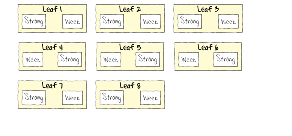
- Note that each level of the Treatment (Strong and Week) are applied to each Leaf (Block)
- Note that Treatments are randomly applied
- The Treatment effect is the mean difference between Treatment pairs per leaf
- Blocking in this way is very useful when spatial or temporal heterogeneity is likely to add noise that could make it difficualt to detect a difference between Treatments. Hence it is a way of experimentally reducing unexplained variation (compared to nesting which involves statistical reduction of unexplained variation).
Since each level of treatment was applied to each leaf, the data represents a randomized block design with leaves as blocks.
The variable LEAF contains a list of Leaf identification numbers and is supposed to represent a factorial blocking variable. However, because the contents of this variable are numbers, R initially treats them as numbers, and therefore considers the variable to be numeric rather than categorical. In order to force R to treat this variable as a factor (categorical) it is necessary to first convert this numeric variable into a factor (HINT).tobacco$LEAF <- as.factor(tobacco$LEAF)
- What are the main hypotheses being tested?
- H0 Factor A:
- H0 Factor B:
- H0 Factor A:
- In the table below, list the assumptions of a randomized block design along with how violations of each assumption are diagnosed and/or the risks of violations are minimized.
-
Assumption Diagnostic/Risk Minimization I. II. III. IV. - Is the proposed model
balanced?
(Yor N)
Show codereplications(NUMBER~LEAF+TREATMENT, data=tobacco)
LEAF TREATMENT 2 8!is.list(replications(NUMBER~LEAF+TREATMENT, data=tobacco))
[1] TRUE
-
- There are a number of
ways of diagnosing block by within block interactions.
- The simplest method is to plot the number of lesions for each treatment and leaf combination (ie. an
interaction plot
(HINT). Any evidence of an interaction? Note that we cannot formally test for an interaction because we don't have replicates for each treatment-leaf combination!
- We can also examine the residual plot from the fitted linear
model. A curvilinear pattern in which the residual values switch from positive to negative
and back again (or visa versa) over the range of predicted values implies that the scale
(magnitude but not polarity) of the main treatment effects differs substantially across the range
of blocks. (HINT). Any evidence of an interaction?
- Perform a Tukey's test for non-additivity evaluated at α = 0.10 or even &alpha = 0.25. This (curvilinear test)
formally tests for the presence of a quadratic trend in the relationship between residuals and
predicted values. As such, it too is only appropriate for simple interactions of scale.
(HINT). Any evidence of an interaction?
- Examine a lattice graphic to determine the consistency of the effect across each of the blocks(HINT).
Show codelibrary(car) interaction.plot(tobacco$LEAF, tobacco$TREATMENT, tobacco$NUMBER)
 Show ggplot code
library(ggplot2)
ggplot(tobacco, aes(y=NUMBER, x=LEAF, group=TREATMENT, color=TREATMENT)) +
  geom_line()
 Show code
residualPlots(lm(NUMBER~LEAF+TREATMENT, data=tobacco))
           Test stat Pr(>|t|)
LEAF              NA       NA
TREATMENT         NA       NA
Tukey test     -0.18    0.858
residualPlots(lm(NUMBER~LEAF+TREATMENT, data=tobacco))

           Test stat Pr(>|t|)
LEAF              NA       NA
TREATMENT         NA       NA
Tukey test     -0.18    0.858
Show codelibrary(alr3) tukey.nonadd.test(lm(NUMBER~LEAF+TREATMENT, data=tobacco))
   Test  Pvalue
-0.1795  0.8575
Show codelibrary(lattice) print(barchart(NUMBER~TREATMENT|LEAF, data=tobacco))

- The simplest method is to plot the number of lesions for each treatment and leaf combination (ie. an
interaction plot
(HINT). Any evidence of an interaction? Note that we cannot formally test for an interaction because we don't have replicates for each treatment-leaf combination!
- Analyse these data with a classic
randomized block ANOVA
(HINT) to test the H0 that there is no difference in the number of lesions produced by the different strength viruses. Complete the table below.
Show code
tobacco.aov <- aov(NUMBER~TREATMENT+Error(LEAF), data=tobacco)
summary(tobacco.aov)
Error: LEAF
          Df Sum Sq Mean Sq F value Pr(>F)
Residuals  7    292    41.7

Error: Within
          Df Sum Sq Mean Sq F value Pr(>F)
TREATMENT  1    248   248.3    17.2 0.0043 **
Residuals  7    101    14.5
---
Signif. codes:
0 '***' 0.001 '**' 0.01 '*' 0.05 '.' 0.1 ' ' 1
Source of variation df Mean Sq F-ratio P-value LEAF (block) TREAT Residuals - Interprete the results.
- Now analyse these data with a linear mixed effects model (REML).
Show lme code
library(nlme)
tobacco.lme <- lme(NUMBER~TREATMENT, random=~1|LEAF, data=tobacco, method='ML')
summary(tobacco.lme)
Linear mixed-effects model fit by maximum likelihood
 Data: tobacco
    AIC   BIC logLik
  102.5 105.6 -47.25

Random effects:
 Formula: ~1 | LEAF
        (Intercept) Residual
StdDev:       3.454    3.557

Fixed effects: NUMBER ~ TREATMENT
              Value Std.Error DF t-value p-value
(Intercept)   34.94     1.874  7  18.645  0.0000
TREATMENTWeak -7.88     1.901  7  -4.144  0.0043
 Correlation:
              (Intr)
TREATMENTWeak -0.507

Standardized Within-Group Residuals:
     Min       Q1      Med       Q3      Max
-1.73025 -0.51798  0.01212  0.43724  1.52636

Number of Observations: 16
Number of Groups: 8
#unique(confint(tobacco.lme,'TREATMENTWeak')[[1]]) library(gmodels) ci(tobacco.lme)
Estimate CI lower CI upper (Intercept) 34.940 30.51 39.371 TREATMENTWeak -7.879 -12.38 -3.383 Std. Error DF p-value (Intercept) 1.874 7 3.169e-07 TREATMENTWeak 1.901 7 4.328e-03anova(tobacco.lme)
            numDF denDF F-value p-value
(Intercept)     1     7   368.5  <.0001
TREATMENT       1     7    17.2  0.0043
Show lmer codelibrary(lme4) tobacco.lmer <- lmer(NUMBER~TREATMENT +(1|LEAF), data=tobacco) summary(tobacco.lmer)
Linear mixed model fit by REML ['lmerMod'] Formula: NUMBER ~ TREATMENT + (1 | LEAF) Data: tobacco REML criterion at convergence: 88.7 Scaled residuals: Min 1Q Median 3Q Max -1.6185 -0.4845 0.0113 0.4090 1.4278 Random effects: Groups Name Variance Std.Dev. LEAF (Intercept) 13.6 3.69 Residual 14.5 3.80 Number of obs: 16, groups: LEAF, 8 Fixed effects: Estimate Std. Error t value (Intercept) 34.94 1.87 18.64 TREATMENTWeak -7.88 1.90 -4.14 Correlation of Fixed Effects: (Intr) TREATMENTWk -0.507anova(tobacco.lmer)
Analysis of Variance Table
          Df Sum Sq Mean Sq F value
TREATMENT  1    248     248    17.2
# Perform SAS-like p-value calculations (requires the lmerTest and pbkrtest package) library(lmerTest) tobacco.lmer <- lmer(NUMBER~TREATMENT +(1|LEAF), data=tobacco) summary(tobacco.lmer)
Linear mixed model fit by REML t-tests use Satterthwaite approximations to degrees of freedom [ merModLmerTest] Formula: NUMBER ~ TREATMENT + (1 | LEAF) Data: tobacco REML criterion at convergence: 88.7 Scaled residuals: Min 1Q Median 3Q Max -1.6185 -0.4845 0.0113 0.4090 1.4278 Random effects: Groups Name Variance Std.Dev. LEAF (Intercept) 13.6 3.69 Residual 14.5 3.80 Number of obs: 16, groups: LEAF, 8 Fixed effects: Estimate Std. Error df t value Pr(>|t|) (Intercept) 34.94 1.87 11.33 18.64 7.4e-10 *** TREATMENTWeak -7.88 1.90 7.00 -4.14 0.0043 ** --- Signif. codes: 0 '***' 0.001 '**' 0.01 '*' 0.05 '.' 0.1 ' ' 1 Correlation of Fixed Effects: (Intr) TREATMENTWk -0.507anova(tobacco.lmer) # Satterthwaite denominator df method
Analysis of Variance Table of type 3 with Satterthwaite approximation for degrees of freedom Sum Sq Mean Sq NumDF DenDF F.value Pr(>F) TREATMENT 248 248 1 7 17.2 0.0043 ** --- Signif. codes: 0 '***' 0.001 '**' 0.01 '*' 0.05 '.' 0.1 ' ' 1anova(tobacco.lmer,ddf="Kenward-Roger") # Kenward-Roger denominator df method
Analysis of Variance Table of type 3  with  Kenward-Roger
approximation for degrees of freedom
          Sum Sq Mean Sq NumDF DenDF F.value Pr(>F)
TREATMENT    248     248     1     7    17.2 0.0043 **
---
Signif. codes:  0 '***' 0.001 '**' 0.01 '*' 0.05 '.' 0.1 ' ' 1
#Examine the effect season via a likelihood ratio test tobacco.lmer1 <- lmer(NUMBER~TREATMENT +(1|LEAF), data=tobacco, REML=F) tobacco.lmer2 <- lmer(NUMBER~1 +(1|LEAF), data=tobacco, REML=F) anova(tobacco.lmer1,tobacco.lmer2, test="F")
Data: tobacco
Models:
..1: NUMBER ~ 1 + (1 | LEAF)
object: NUMBER ~ TREATMENT + (1 | LEAF)
       Df AIC BIC logLik deviance Chisq Chi Df Pr(>Chisq)
..1     3 110 113  -52.2    104.5
object  4 102 106  -47.2     94.5  9.98      1     0.0016 **
---
Signif. codes:  0 '***' 0.001 '**' 0.01 '*' 0.05 '.' 0.1 ' ' 1
Show ezANOVA codelibrary(ez) ezANOVA(dv=.(NUMBER),within=.(TREATMENT),wid=.(LEAF), data=tobacco,type=3)
$ANOVA Effect DFn DFd F p p<.05 ges 2 TREATMENT 1 7 17.17 0.004328 * 0.387 - Generate a summary figure with predicted mean number of lesions (and confidence interval) for each treatment.
Show code
newdata <- expand.grid(TREATMENT=c("STRONG","WEAK"), NUMBER=0)
Xmat <- model.matrix(terms(tobacco.lmer),newdata)
Xmat
  (Intercept) TREATMENTWEAK
1           1             0
2           1             1
attr(,"assign")
[1] 0 1
attr(,"contrasts")
attr(,"contrasts")$TREATMENT
[1] "contr.treatment"
pred <- as.vector(fixef(tobacco.lmer) %*% t(Xmat))
se <- sqrt(diag(Xmat %*% vcov(tobacco.lmer) %*% t(Xmat)))
newdata$fit <- pred
newdata$lower <- pred - 2*se
newdata$upper <- pred + 2*se

library(ggplot2)
library(grid)
ggplot(newdata, aes(y=fit, x=TREATMENT)) +
  geom_errorbar(aes(ymin=lower, ymax=upper), width=0.01)+
  geom_point() +
  scale_x_discrete('Inoculation treatment')+
  scale_y_continuous('Number of lesions')+
  theme_classic() +
  theme(axis.title.y=element_text(vjust=2,size=rel(1.2)),
        axis.title.x=element_text(vjust=-2,size=rel(1.2)),
        plot.margin=unit(c(0.5,0.5,2,2),'lines'))

ggplot(newdata, aes(y=fit, x=TREATMENT)) +
  geom_bar(stat='identity', fill='grey', color='black') +
  geom_errorbar(aes(ymin=lower, ymax=upper), width=0.01)+
  scale_x_discrete('Inoculation treatment')+
  scale_y_continuous('Number of lesions', expand=c(0,0))+
  theme_classic() +
  theme(axis.title.y=element_text(vjust=2,size=rel(1.2)),
        axis.title.x=element_text(vjust=-2,size=rel(1.2)),
        plot.margin=unit(c(0.5,0.5,2,2),'lines'))
