Workshop 7.4a - Split-plot and complex repeated measures designs (mixed effects models)
30 Jan 2015
ANCOVA references
- Logan (2010) - Chpt 12-14
- Quinn & Keough (2002) - Chpt 9-11
Very basic overview of Randomized block
Split-plot
Split-plotIn an attempt to understand the effects on marine animals of short-term exposure to toxic substances, such as might occur following a spill, or a major increase in storm water flows, a it was decided to examine the toxicant in question, Copper, as part of a field experiment in Honk Kong. The experiment consisted of small sources of Cu (small, hemispherical plaster blocks, impregnated with copper), which released the metal into sea water over 4 or 5 days. The organism whose response to Cu was being measured was a small, polychaete worm, Hydroides, that attaches to hard surfaces in the sea, and is one of the first species to colonize any surface that is submerged. The biological questions focused on whether the timing of exposure to Cu affects the overall abundance of these worms. The time period of interest was the first or second week after a surface being available.
The experimental setup consisted of sheets of black perspex (settlement plates), which provided good surfaces for these worms. Each plate had a plaster block bolted to its centre, and the dissolving block would create a gradient of [Cu] across the plate. Over the two weeks of the experiment, a given plate would have pl ain plaster blocks (Control) or a block containing copper in the first week, followed by a plain block, or a plain block in the first week, followed by a dose of copper in the second week. After two weeks in the water, plates were removed and counted back in the laboratory. Without a clear idea of how sensitive these worms are to copper, an effect of the treatments might show up as an overall difference in the density of worms across a plate, or it could show up as a gradient in abundance across the plate, with a different gradient in different treatments. Therefore, on each plate, the density of worms (#/cm2) was recorded at each of four distances from the center of the plate.
Download Copper data set| Format of copper.csv data file | |||||||||||||||||
|---|---|---|---|---|---|---|---|---|---|---|---|---|---|---|---|---|---|
|
 |
copper <- read.table('../downloads/data/copper.csv', header=T, sep=',', strip.white=T)
head(copper)
   COPPER PLATE DIST WORMS
1 control   200    4 11.50
2 control   200    3 13.00
3 control   200    2 13.50
4 control   200    1 12.00
5 control    39    4 17.75
6 control    39    3 13.75
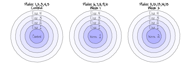
The Plates are the "random" groups. Within each Plate, all levels of the Distance factor occur (this is a within group factor). Each Plate can only be of one of the three levels of the Copper treatment. This is therefore a within group (nested) factor. Traditionally, this mixture of nested and randomized block design would be called a partly nested or split-plot design.
Notice that both the PLATE variable and the DIST variable contain only numbers. Make sure that you define both of these as factors (HINT)copper$PLATE <- factor(copper$PLATE) copper$DIST <- factor(copper$DIST)
- What are the main hypotheses being tested?
- H0 Main Effect 1 (Factor A):
- H0 Main Effect 2 (Factor C):
- H0 Main Effect 3 (A*C):
- H0 Main Effect 1 (Factor A):
- The usual ANOVA assumptions apply to split-plot designs, and these can be tested by constructing boxplots for each of the main effects. However, it is important to consider what data the boxplots should be based upon. For each of the main hypothesis tests, describe what data should be used to construct boxplots (remember that the assumptions of normality and homogeneity of variance apply to the residuals of each hypothesis test, and therefore the data used in the construction of boxplots for each hypothesis test should represent the respective residuals, or sources of unexplained variation).
- H0 Main Effect 1 (Factor A):
- H0 Main Effect 2 (Factor C):
- H0 Main Effect 3 (A*C):
- H0 Main Effect 1 (Factor A):
- For each of the hypothesis tests, indicate which Mean Square term should be used as the residual (denominator) in the F-ratio calculation.
Note, COPPER and DIST are fixed factors and PLATE is a random factor.
- H0 Main Effect 1 (Factor A): F-ratio = MSCOPPER/MS
- H0 Main Effect 2 (Factor C): F-ratio = MSDIST/MS
- H0 Main Effect 3 (A*C): F-ratio = MSCOPPER:DIST/MS
- H0 Main Effect 1 (Factor A): F-ratio = MSCOPPER/MS
- Construct a boxplot to investigate the assumptions as they apply to the test of H0 Main Effect 1 (Factor A): This is done in two steps
- Aggregate the data set by the mean number of WORMS within each plate (HINT)
- Construct a boxplot of aggregated mean number of WORMS against COPPER treatment (HINT)
- Any evidence of violations of the assumptions (y or n)?
Show codelibrary(plyr) cu.ag <- ddply(copper,~COPPER+PLATE, function(df) data.frame(WORMS=mean(df$WORMS))) #OR library(plyr) cu.ag <-ddply(copper, ~COPPER+PLATE, summarise, WORMS = mean(WORMS, na.rm = TRUE)) #OR cu.ag <- aggregate(copper,list(COPPER=copper$COPPER, PLATE=copper$PLATE), mean) #OR library(nlme) cu.ag <- gsummary(copper,form=~COPPER/PLATE, base:::mean)
Show codeboxplot(WORMS ~ COPPER, data=cu.ag)
 Show ggplot code
library(ggplot2)
ggplot(cu.ag, aes(y=WORMS, x=COPPER)) + geom_boxplot()

- Construct a boxplot to investigate the assumptions as they apply to the test of H0 Main Effect 2 (Factor C): Since Factor C is tested against the overal residual in this case, this is a relatively straight forward procedure.
(HINT)
Show codeboxplot(WORMS ~ DIST, data=copper)
 Show ggplot code
library(ggplot2)
ggplot(copper, aes(y=WORMS, x=DIST)) + geom_boxplot()

- Any evidence of violations of the assumptions (y or n)?
- Any evidence of violations of the assumptions (y or n)?
- Construct a boxplot to investigate the assumptions as they apply to the test of H0 the main interaction effect (A:C): Since A:C is tested against the overal residual, this is a relatively straight forward procedure.(HINT)
Show code
boxplot(WORMS ~ COPPER:DIST, data=copper)
 Show ggplot code
library(ggplot2)
ggplot(copper, aes(y=WORMS, x=DIST, color=COPPER)) + geom_boxplot()

- Any evidence of violations of the assumptions (y or n)?
- Any evidence of violations of the assumptions (y or n)?
- In addition to the above assumptions, the test of PLATE assumes that there is no PLATE by DIST interaction as this is the overal residual (the replicates).
That is, the test assumes that the effect of DIST is consistent in all PLATES.
Construct an interaction plot to examine whether there is any evidence of an interaction between PLATE and DISTANCE
(HINT)
Show code
library(car)
with(copper,interaction.plot(PLATE, DIST, WORMS))

library(ggplot2)
ggplot(copper, aes(y=WORMS, x=as.numeric(PLATE), color=DIST)) + geom_line(stat='summary', fun.y=mean)

library(alr3)
tukey.nonadd.test(lm(WORMS~PLATE+DIST, data=copper))
      Test     Pvalue
-4.122e+00  3.749e-05
- Any evidence of an interaction (y or n)?
- Is the design (model)
unbalanced ?
(HINT) (Yor N) Show code
replications(WORMS ~ COPPER + Error(PLATE) + DIST +COPPER:DIST,data=copper)
COPPER DIST COPPER:DIST 20 15 5!is.list(replications(WORMS ~ COPPER + Error(PLATE) + DIST +COPPER:DIST,data=copper))
[1] TRUE
- Is there any evidence of issues with
sphericity
?(HINT) (Y or N)
- Any issue with autocorrelation?
?(HINT) (Y or N)
Show codelibrary(biology) epsi.GG.HF(aov(WORMS ~ COPPER + Error(PLATE) + DIST +COPPER:DIST,data=copper))
$GG.eps
[1] 0.5203

$HF.eps
[1] 0.5841

$sigma
[1] 1.807
Show codelibrary(nlme) acf(resid(lme(WORMS~COPPER*DIST, random=~1|PLATE, data=copper)))

- Any evidence of an interaction (y or n)?
- Write out the linear model
- Perform a
split-plot ANOVA
(HINT).
Show code
copper.aov <- aov(WORMS ~ COPPER + DIST + COPPER:DIST + Error(PLATE), data=copper)
- Using linear mixed effects (lme) model. It is a good idea to fit a range of models (random intercept, random intercept/slope, alternative correlations structures)
and use selection criterion (such as AIC) to determine which candidate model fits the data best.
Show code
library(nlme)
# fit random intercepts model
copper.lme <- lme(WORMS ~ COPPER*DIST, random=~1|PLATE, data=copper, method='REML')
# fit random intercepts and slopes model
copper.lme1 <- lme(WORMS ~ COPPER*DIST, random=~DIST|PLATE, data=copper, method='REML')
AIC(copper.lme, copper.lme1)
            df   AIC
copper.lme  14 218.3
copper.lme1 23 217.4
anova(copper.lme, copper.lme1)
            Model df   AIC   BIC logLik   Test L.Ratio p-value
copper.lme      1 14 218.2 244.4 -95.13
copper.lme1     2 23 217.4 260.4 -85.69 1 vs 2   18.88  0.0262
copper.lme.AR1 <- lme(WORMS ~ COPPER*DIST, random=~1|PLATE, data=copper, method='REML',
   correlation=corAR1(form=~1|PLATE))
AIC(copper.lme, copper.lme1, copper.lme.AR1)
               df   AIC
copper.lme     14 218.3
copper.lme1    23 217.4
copper.lme.AR1 15 214.4
anova(copper.lme, copper.lme.AR1, copper.lme1)
               Model df   AIC   BIC logLik   Test L.Ratio p-value
copper.lme         1 14 218.2 244.4 -95.13
copper.lme.AR1     2 15 214.4 242.4 -92.19 1 vs 2   5.881  0.0153
copper.lme1        3 23 217.4 260.4 -85.69 2 vs 3  12.997  0.1119
# Conclusions: the random intercepts/slopes model does account a little for the some of the extra variance in the model,
# however incorporating first order autoregressive correlation structure fits the data even better.
# Arguably, the source of the additional variance is likely to be due to autocorrelation and thus incorporating the
# the autoregressive structure is the 'best' solution.
- Using linear mixed effects (lmer) model. It is a good idea to fit a range of models (random intercept, random intercept/slope, alternative correlations structures)
and use selection criterion (such as AIC) to determine which candidate model fits the data best.
Show code
library(lme4)
# fit random intercepts model
copper.lmer <- lmer(WORMS ~ COPPER*DIST+(1|PLATE), data=copper, REML=TRUE)
# fit random intercepts and slopes model
copper.lmer1 <- lmer(WORMS ~ COPPER*DIST+(DIST|PLATE), data=copper, REML=TRUE,
  control=lmerControl(check.nobs.vs.nRE="ignore"))
copper.lmer2 <- lmer(WORMS ~ COPPER*DIST+(COPPER|PLATE), data=copper, REML=TRUE,
  control=lmerControl(check.nobs.vs.nRE="ignore"))
copper.lmer3 <- lmer(WORMS ~ COPPER*DIST+(DIST|PLATE)+(COPPER|PLATE), data=copper, REML=TRUE,
  control=lmerControl(check.nobs.vs.nRE="ignore"))

AIC(copper.lmer, copper.lmer1, copper.lmer2, copper.lmer3)
             df   AIC
copper.lmer  14 218.3
copper.lmer1 23 217.4
copper.lmer2 19 225.4
copper.lmer3 29 225.3
anova(copper.lmer, copper.lmer1, copper.lmer2, copper.lmer3)
Data: copper
Models:
copper.lmer: WORMS ~ COPPER * DIST + (1 | PLATE)
copper.lmer2: WORMS ~ COPPER * DIST + (COPPER | PLATE)
copper.lmer1: WORMS ~ COPPER * DIST + (DIST | PLATE)
copper.lmer3: WORMS ~ COPPER * DIST + (DIST | PLATE) + (COPPER | PLATE)
             Df AIC BIC logLik deviance Chisq Chi Df Pr(>Chisq)
copper.lmer  14 228 258 -100.1      200
copper.lmer2 19 235 274  -98.4      197  3.56      5    0.61403
copper.lmer1 23 223 271  -88.3      177 20.04      4    0.00049 ***
copper.lmer3 29 230 290  -85.8      172  5.08      6    0.53409
---
Signif. codes:  0 '***' 0.001 '**' 0.01 '*' 0.05 '.' 0.1 ' ' 1
# Conclusions: without the ability to incorporate alternative correlation structures, the only means to attempt # to account for extra variability is to use random intercepts/slopes models. # In this case, arguably the second model is 'best'.
- Explore a range of model diagnostics
- Construct an
interaction plot
showing the density of worms against distance from Cu source, with each treatment as different lines (or different bars).
HINT
Show code
interaction.plot(copper$DIST, copper$COPPER, copper$WORMS)
 Show code
library(effects)
plot(allEffects(copper.lme.AR1))

plot(allEffects(copper.lme.AR1), multiline=TRUE)

- Residual plots
Show code
# Traditional ANOVA
par(mfrow=c(2,2))
plot(lm(copper.aov))

# LME
plot(copper.lme.AR1)

plot(residuals(copper.lme.AR1, type='normalized') ~ fitted(copper.lme.AR1))
plot(residuals(copper.lme.AR1, type='normalized') ~ copper$COPPER)
plot(residuals(copper.lme.AR1, type='normalized') ~ copper$DIST)
plot(residuals(copper.lme.AR1, type='normalized') ~ interaction(copper$COPPER,copper$DIST))

#LMER
par(mfrow=c(1,1))
plot(copper.lmer1)

par(mfrow=c(2,2))
plot(resid(copper.lmer1) ~ copper$COPPER)
plot(resid(copper.lmer1) ~ copper$DIST)
plot(resid(copper.lmer1) ~ interaction(copper$COPPER,copper$DIST))

- Construct an
interaction plot
showing the density of worms against distance from Cu source, with each treatment as different lines (or different bars).
HINT
- Explore the model parameters
- Traditional ANOVA and
complete the following table (HINT).
To obtain the hypothesis test for the random factor (Factor B: PLATE), run the model as if all factors were fixed and thus all terms are tested against the overall residuals,
HINT).
Source of variation df Mean Sq F-ratio P-value COPPER PLATE DIST COPPER:DIST Residuals Show codesummary(copper.aov)
Error: PLATE Df Sum Sq Mean Sq F value Pr(>F) COPPER 2 784 392 128 8.1e-09 *** Residuals 12 37 3 --- Signif. codes: 0 '***' 0.001 '**' 0.01 '*' 0.05 '.' 0.1 ' ' 1 Error: Within Df Sum Sq Mean Sq F value Pr(>F) DIST 3 153.8 51.3 28.38 1.4e-09 *** COPPER:DIST 6 53.4 8.9 4.93 9e-04 *** Residuals 36 65.0 1.8 --- Signif. codes: 0 '***' 0.001 '**' 0.01 '*' 0.05 '.' 0.1 ' ' 1library(biology) AnovaM(copper.aov, RM=TRUE)
   Sphericity Epsilon Values
-------------------------------
 Greenhouse.Geisser Huynh.Feldt
             0.5203      0.5841
Anova Table (Type I tests) Response: WORMS Error: PLATE Df Sum Sq Mean Sq F value Pr(>F) COPPER 2 784 392 128 8.1e-09 *** Residuals 12 37 3 --- Signif. codes: 0 '***' 0.001 '**' 0.01 '*' 0.05 '.' 0.1 ' ' 1 Error: Within Df Sum Sq Mean Sq F value Pr(>F) DIST 3 153.8 51.3 28.38 1.4e-09 *** COPPER:DIST 6 53.4 8.9 4.93 9e-04 *** Residuals 36 65.0 1.8 --- Signif. codes: 0 '***' 0.001 '**' 0.01 '*' 0.05 '.' 0.1 ' ' 1 Greenhouse-Geisser corrected ANOVA table Response: WORMS Error: PLATE Df Sum Sq Mean Sq F value Pr(>F) COPPER 1.04 784 392 128 8e-08 *** Residuals 12.00 37 3 --- Signif. codes: 0 '***' 0.001 '**' 0.01 '*' 0.05 '.' 0.1 ' ' 1 Error: Within Df Sum Sq Mean Sq F value Pr(>F) DIST 1.56 153.8 51.3 28.38 2.7e-07 *** COPPER:DIST 3.12 53.4 8.9 4.93 0.0052 ** Residuals 36.00 65.0 1.8 --- Signif. codes: 0 '***' 0.001 '**' 0.01 '*' 0.05 '.' 0.1 ' ' 1 Huynh-Feldt corrected ANOVA table Response: WORMS Error: PLATE Df Sum Sq Mean Sq F value Pr(>F) COPPER 1.17 784 392 128 5.3e-08 *** Residuals 12.00 37 3 --- Signif. codes: 0 '***' 0.001 '**' 0.01 '*' 0.05 '.' 0.1 ' ' 1 Error: Within Df Sum Sq Mean Sq F value Pr(>F) DIST 1.75 153.8 51.3 28.38 1.1e-07 *** COPPER:DIST 3.50 53.4 8.9 4.93 0.004 ** Residuals 36.00 65.0 1.8 --- Signif. codes: 0 '***' 0.001 '**' 0.01 '*' 0.05 '.' 0.1 ' ' 1 - LME
- LMER
Show codesummary(copper.lme.AR1)
Linear mixed-effects model fit by REML Data: copper AIC BIC logLik 214.4 242.4 -92.19 Random effects: Formula: ~1 | PLATE (Intercept) Residual StdDev: 0.0001127 1.469 Correlation Structure: AR(1) Formula: ~1 | PLATE Parameter estimate(s): Phi 0.448 Fixed effects: WORMS ~ COPPER * DIST Value Std.Error DF t-value p-value (Intercept) 10.85 0.6568 36 16.518 0.0000 COPPERWeek 1 -3.60 0.9289 12 -3.875 0.0022 COPPERWeek 2 -10.60 0.9289 12 -11.411 0.0000 DIST2 1.15 0.6902 36 1.666 0.1043 DIST3 1.55 0.8305 36 1.866 0.0702 DIST4 2.70 0.8862 36 3.047 0.0043 COPPERWeek 1:DIST2 -0.05 0.9760 36 -0.051 0.9594 COPPERWeek 2:DIST2 0.05 0.9760 36 0.051 0.9594 COPPERWeek 1:DIST3 -0.30 1.1745 36 -0.255 0.7998 COPPERWeek 2:DIST3 2.20 1.1745 36 1.873 0.0692 COPPERWeek 1:DIST4 0.05 1.2532 36 0.040 0.9684 COPPERWeek 2:DIST4 4.90 1.2532 36 3.910 0.0004 Correlation: (Intr) COPPERWk1 COPPERWk2 DIST2 DIST3 DIST4 COPPERW1:DIST2 COPPERW2:DIST2 COPPERWeek 1 -0.707 COPPERWeek 2 -0.707 0.500 DIST2 -0.525 0.371 0.371 DIST3 -0.632 0.447 0.447 0.602 DIST4 -0.675 0.477 0.477 0.468 0.678 COPPERWeek 1:DIST2 0.371 -0.525 -0.263 -0.707 -0.425 -0.331 COPPERWeek 2:DIST2 0.371 -0.263 -0.525 -0.707 -0.425 -0.331 0.500 COPPERWeek 1:DIST3 0.447 -0.632 -0.316 -0.425 -0.707 -0.480 0.602 0.301 COPPERWeek 2:DIST3 0.447 -0.316 -0.632 -0.425 -0.707 -0.480 0.301 0.602 COPPERWeek 1:DIST4 0.477 -0.675 -0.337 -0.331 -0.480 -0.707 0.468 0.234 COPPERWeek 2:DIST4 0.477 -0.337 -0.675 -0.331 -0.480 -0.707 0.234 0.468 COPPERW1:DIST3 COPPERW2:DIST3 COPPERW1:DIST4 COPPERWeek 1 COPPERWeek 2 DIST2 DIST3 DIST4 COPPERWeek 1:DIST2 COPPERWeek 2:DIST2 COPPERWeek 1:DIST3 COPPERWeek 2:DIST3 0.500 COPPERWeek 1:DIST4 0.678 0.339 COPPERWeek 2:DIST4 0.339 0.678 0.500 Standardized Within-Group Residuals: Min Q1 Med Q3 Max -1.3958 -0.5957 -0.1702 0.5362 2.8596 Number of Observations: 60 Number of Groups: 15anova(copper.lme.AR1)
            numDF denDF F-value p-value
(Intercept)     1    36   980.6  <.0001
COPPER          2    12    93.1  <.0001
DIST            3    36    25.1  <.0001
COPPER:DIST     6    36     4.3  0.0025
intervals(copper.lme.AR1)
Approximate 95% confidence intervals Fixed effects: lower est. upper (Intercept) 9.5179 10.85 12.182 COPPERWeek 1 -5.6239 -3.60 -1.576 COPPERWeek 2 -12.6239 -10.60 -8.576 DIST2 -0.2497 1.15 2.550 DIST3 -0.1343 1.55 3.234 DIST4 0.9028 2.70 4.497 COPPERWeek 1:DIST2 -2.0295 -0.05 1.929 COPPERWeek 2:DIST2 -1.9295 0.05 2.029 COPPERWeek 1:DIST3 -2.6820 -0.30 2.082 COPPERWeek 2:DIST3 -0.1820 2.20 4.582 COPPERWeek 1:DIST4 -2.4917 0.05 2.592 COPPERWeek 2:DIST4 2.3583 4.90 7.442 attr(,"label") [1] "Fixed effects:" Random Effects: Level: PLATE lower est. upper sd((Intercept)) 0 0.0001127 Inf Correlation structure: lower est. upper Phi 0.1184 0.448 0.6887 attr(,"label") [1] "Correlation structure:" Within-group standard error: lower est. upper 1.162 1.469 1.857Show codelibrary(lmerTest) copper.lmer <- update(copper.lmer1) summary(copper.lmer)
Linear mixed model fit by REML ['merModLmerTest'] Formula: WORMS ~ COPPER * DIST + (DIST | PLATE) Data: copper Control: lmerControl(check.nobs.vs.nRE = "ignore") REML criterion at convergence: 171.4 Scaled residuals: Min 1Q Median 3Q Max -2.044 -0.358 0.006 0.314 1.772 Random effects: Groups Name Variance Std.Dev. Corr PLATE (Intercept) 0.739 0.860 DIST2 0.222 0.471 0.63 DIST3 1.803 1.343 -0.56 -0.69 DIST4 4.185 2.046 -0.46 -0.91 0.87 Residual 0.434 0.659 Number of obs: 60, groups: PLATE, 15 Fixed effects: Estimate Std. Error t value (Intercept) 10.850 0.484 22.40 COPPERWeek 1 -3.600 0.685 -5.26 COPPERWeek 2 -10.600 0.685 -15.48 DIST2 1.150 0.467 2.46 DIST3 1.550 0.731 2.12 DIST4 2.700 1.005 2.69 COPPERWeek 1:DIST2 -0.050 0.660 -0.08 COPPERWeek 2:DIST2 0.050 0.660 0.08 COPPERWeek 1:DIST3 -0.300 1.034 -0.29 COPPERWeek 2:DIST3 2.200 1.034 2.13 COPPERWeek 1:DIST4 0.050 1.422 0.04 COPPERWeek 2:DIST4 4.900 1.422 3.45 Correlation of Fixed Effects: (Intr) COPPERWk1 COPPERWk2 DIST2 DIST3 DIST4 COPPERW1:DIST2 COPPERW2:DIST2 COPPERWeek1 -0.707 COPPERWeek2 -0.707 0.500 DIST2 -0.158 0.111 0.111 DIST3 -0.613 0.434 0.434 -0.002 DIST4 -0.513 0.362 0.362 -0.191 0.770 COPPERW1:DIST2 0.111 -0.158 -0.079 -0.707 0.001 0.135 COPPERW2:DIST2 0.111 -0.079 -0.158 -0.707 0.001 0.135 0.500 COPPERW1:DIST3 0.434 -0.613 -0.307 0.001 -0.707 -0.545 -0.002 -0.001 COPPERW2:DIST3 0.434 -0.307 -0.613 0.001 -0.707 -0.545 -0.001 -0.002 COPPERW1:DIST4 0.362 -0.513 -0.256 0.135 -0.545 -0.707 -0.191 -0.095 COPPERW2:DIST4 0.362 -0.256 -0.513 0.135 -0.545 -0.707 -0.095 -0.191 COPPERW1:DIST3 COPPERW2:DIST3 COPPERW1:DIST4 COPPERWeek1 COPPERWeek2 DIST2 DIST3 DIST4 COPPERW1:DIST2 COPPERW2:DIST2 COPPERW1:DIST3 COPPERW2:DIST3 0.500 COPPERW1:DIST4 0.770 0.385 COPPERW2:DIST4 0.385 0.770 0.500anova(copper.lmer, ddf='Satterthwaite')
Analysis of Variance Table Df Sum Sq Mean Sq F value COPPER 2 143.6 71.8 165.52 DIST 3 41.4 13.8 31.80 COPPER:DIST 6 7.6 1.3 2.93anova(copper.lmer, ddf='Kenward-Roger')
Analysis of Variance Table of type 3  with  Kenward-Roger
approximation for degrees of freedom
            Sum Sq Mean Sq NumDF DenDF F.value  Pr(>F)
COPPER       111.0    55.5     2    12   128.0 8.1e-09 ***
DIST          34.5    11.5     3    10    26.5 4.5e-05 ***
COPPER:DIST    6.1     1.0     6    12     2.3   0.099 .
---
Signif. codes:  0 '***' 0.001 '**' 0.01 '*' 0.05 '.' 0.1 ' ' 1
- Traditional ANOVA and
complete the following table (HINT).
To obtain the hypothesis test for the random factor (Factor B: PLATE), run the model as if all factors were fixed and thus all terms are tested against the overall residuals,
HINT).
- In order to tease out the interaction, we could analyse the effects of the main factor (COPPER) separately for each Distance and/or investigate the effects of Distance separately for each of the three copper treatments.
Recall that when performing such simple main effects, it is necessary to use the residual terms from the global analyses as these are likely to be better estimates (as they are based on a larger amount of data).
- Investigate the effects of copper separately for each of the
four distances HINT
- Traditional ANOVA
Show code
AnovaM(mainEffects(copper.aov, at=DIST==1),type='III')
Error: PLATE Df Sum Sq Mean Sq F value Pr(>F) INT 2 784 392 128 8.1e-09 *** Residuals 12 37 3 --- Signif. codes: 0 '***' 0.001 '**' 0.01 '*' 0.05 '.' 0.1 ' ' 1 Error: Within Df Sum Sq Mean Sq F value Pr(>F) INT 9 207 23.02 12.7 8.4e-09 *** Residuals 36 65 1.81 --- Signif. codes: 0 '***' 0.001 '**' 0.01 '*' 0.05 '.' 0.1 ' ' 1AnovaM(mainEffects(copper.aov, at=DIST==2),type='III')
Error: PLATE Df Sum Sq Mean Sq F value Pr(>F) INT 2 784 392 128 8.1e-09 *** Residuals 12 37 3 --- Signif. codes: 0 '***' 0.001 '**' 0.01 '*' 0.05 '.' 0.1 ' ' 1 Error: Within Df Sum Sq Mean Sq F value Pr(>F) INT 9 207 23.02 12.7 8.4e-09 *** Residuals 36 65 1.81 --- Signif. codes: 0 '***' 0.001 '**' 0.01 '*' 0.05 '.' 0.1 ' ' 1AnovaM(mainEffects(copper.aov, at=DIST==3),type='III')
Error: PLATE Df Sum Sq Mean Sq F value Pr(>F) INT 2 784 392 128 8.1e-09 *** Residuals 12 37 3 --- Signif. codes: 0 '***' 0.001 '**' 0.01 '*' 0.05 '.' 0.1 ' ' 1 Error: Within Df Sum Sq Mean Sq F value Pr(>F) INT 9 207 23.02 12.7 8.4e-09 *** Residuals 36 65 1.81 --- Signif. codes: 0 '***' 0.001 '**' 0.01 '*' 0.05 '.' 0.1 ' ' 1 - LME
Show code
copper<-within(copper,{COPPER2=ifelse(DIST=='1', '1',as.character(COPPER))})
copper<-within(copper,{CD=interaction(COPPER2,DIST)})
anova(update(copper.lme.AR1, ~CD + . - DIST - COPPER:DIST), type='marginal')
            numDF denDF F-value p-value
(Intercept)     1    36  272.86  <.0001
CD              9    36   11.21  <.0001
COPPER          2    12   67.34  <.0001
copper<-within(copper,{COPPER2=ifelse(DIST=='2', '1',as.character(COPPER))})
copper<-within(copper,{CD=interaction(COPPER2,DIST)})
anova(update(copper.lme.AR1, ~CD + . - DIST - COPPER:DIST), type='marginal')
            numDF denDF F-value p-value
(Intercept)     1    36  272.86  <.0001
CD              9    36   11.21  <.0001
COPPER          2    12   66.53  <.0001
copper<-within(copper,{COPPER2=ifelse(DIST=='3', '1',as.character(COPPER))})
copper<-within(copper,{CD=interaction(COPPER2,DIST)})
anova(update(copper.lme.AR1, ~CD + . - DIST - COPPER:DIST), type='marginal')
            numDF denDF F-value p-value
(Intercept)     1    36  272.86  <.0001
CD              9    36   11.21  <.0001
COPPER          2    12   40.96  <.0001
copper<-within(copper,{COPPER2=ifelse(DIST=='4', '1',as.character(COPPER))})
copper<-within(copper,{CD=interaction(COPPER2,DIST)})
anova(update(copper.lme.AR1, ~CD + . - DIST - COPPER:DIST), type='marginal')
            numDF denDF F-value p-value
(Intercept)     1    36  272.86  <.0001
CD              9    36   11.21  <.0001
COPPER          2    12   19.21   2e-04
- LMER
Show code
copper<-within(copper,{COPPER2=ifelse(DIST=='1', '1',as.character(COPPER))})
copper<-within(copper,{CD=interaction(COPPER2,DIST)})
anova(update(copper.lmer1, ~CD + . - DIST - COPPER:DIST), ddf='Kenward-Roger')
Analysis of Variance Table of type 3 with Kenward-Roger approximation for degrees of freedom Sum Sq Mean Sq NumDF DenDF F.value Pr(>F) CD 38.7 4.3 9 12.8 9.9 0.00018 *** COPPER 107.4 53.7 2 12.0 123.9 9.7e-09 *** --- Signif. codes: 0 '***' 0.001 '**' 0.01 '*' 0.05 '.' 0.1 ' ' 1copper<-within(copper,{COPPER2=ifelse(DIST=='2', '1',as.character(COPPER))}) copper<-within(copper,{CD=interaction(COPPER2,DIST)}) anova(update(copper.lmer1, ~CD + . - DIST - COPPER:DIST), ddf='Kenward-Roger')
Analysis of Variance Table of type 3 with Kenward-Roger approximation for degrees of freedom Sum Sq Mean Sq NumDF DenDF F.value Pr(>F) CD 38.6 4.3 9 12.8 9.9 0.00018 *** COPPER 65.2 32.6 2 12.0 75.3 1.6e-07 *** --- Signif. codes: 0 '***' 0.001 '**' 0.01 '*' 0.05 '.' 0.1 ' ' 1copper<-within(copper,{COPPER2=ifelse(DIST=='3', '1',as.character(COPPER))}) copper<-within(copper,{CD=interaction(COPPER2,DIST)}) anova(update(copper.lmer1, ~CD + . - DIST - COPPER:DIST), ddf='Kenward-Roger')
Analysis of Variance Table of type 3 with Kenward-Roger approximation for degrees of freedom Sum Sq Mean Sq NumDF DenDF F.value Pr(>F) CD 38.7 4.3 9 12.8 9.9 0.00018 *** COPPER 45.8 22.9 2 12.0 52.8 1.1e-06 *** --- Signif. codes: 0 '***' 0.001 '**' 0.01 '*' 0.05 '.' 0.1 ' ' 1copper<-within(copper,{COPPER2=ifelse(DIST=='4', '1',as.character(COPPER))}) copper<-within(copper,{CD=interaction(COPPER2,DIST)}) anova(update(copper.lmer1, ~CD + . - DIST - COPPER:DIST), ddf='Kenward-Roger')
Analysis of Variance Table of type 3  with  Kenward-Roger
approximation for degrees of freedom
       Sum Sq Mean Sq NumDF DenDF F.value  Pr(>F)
CD       38.7    4.30     9  12.8    9.91 0.00018 ***
COPPER    9.6    4.82     2  12.0   11.11 0.00186 **
---
Signif. codes:  0 '***' 0.001 '**' 0.01 '*' 0.05 '.' 0.1 ' ' 1
What conclusions would you draw from these four analyses?
- Traditional ANOVA
- Investigate the effects of distance separately for each of the three copper treatments
- Tranditional ANOVA
HINT
Show code
AnovaM(mainEffects(copper.aov, at=COPPER=='control'),type='III')
Error: PLATE Df Sum Sq Mean Sq F value Pr(>F) INT 2 784 392 128 8.1e-09 *** Residuals 12 37 3 --- Signif. codes: 0 '***' 0.001 '**' 0.01 '*' 0.05 '.' 0.1 ' ' 1 Error: Within Df Sum Sq Mean Sq F value Pr(>F) INT 6 188.6 31.43 17.40 2.5e-09 *** DIST 3 18.6 6.21 3.44 0.027 * Residuals 36 65.0 1.81 --- Signif. codes: 0 '***' 0.001 '**' 0.01 '*' 0.05 '.' 0.1 ' ' 1AnovaM(mainEffects(copper.aov, at=COPPER=='Week 1'),type='III')
Error: PLATE Df Sum Sq Mean Sq F value Pr(>F) INT 2 784 392 128 8.1e-09 *** Residuals 12 37 3 --- Signif. codes: 0 '***' 0.001 '**' 0.01 '*' 0.05 '.' 0.1 ' ' 1 Error: Within Df Sum Sq Mean Sq F value Pr(>F) INT 6 188.1 31.34 17.35 2.6e-09 *** DIST 3 19.2 6.39 3.54 0.024 * Residuals 36 65.0 1.81 --- Signif. codes: 0 '***' 0.001 '**' 0.01 '*' 0.05 '.' 0.1 ' ' 1AnovaM(mainEffects(copper.aov, at=COPPER=='Week 2'),type='III')
Error: PLATE Df Sum Sq Mean Sq F value Pr(>F) INT 2 784 392 128 8.1e-09 *** Residuals 12 37 3 --- Signif. codes: 0 '***' 0.001 '**' 0.01 '*' 0.05 '.' 0.1 ' ' 1 Error: Within Df Sum Sq Mean Sq F value Pr(>F) INT 6 37.8 6.3 3.49 0.0081 ** DIST 3 169.4 56.5 31.26 4e-10 *** Residuals 36 65.0 1.8 --- Signif. codes: 0 '***' 0.001 '**' 0.01 '*' 0.05 '.' 0.1 ' ' 1 - LME
Show code
copper<-within(copper,{DIST2=ifelse(COPPER=='control', '1',as.character(DIST))})
copper<-within(copper,{CD=interaction(DIST2,COPPER)})
anova(update(copper.lme.AR1, ~CD + . - COPPER - COPPER:DIST), type='marginal')
            numDF denDF F-value p-value
(Intercept)     1    34  272.86  <.0001
CD              8    34   26.45  <.0001
DIST            3    34    3.18  0.0361
copper<-within(copper,{DIST2=ifelse(COPPER=='Week 1', '1',as.character(DIST))})
copper<-within(copper,{CD=interaction(DIST2,COPPER)})
anova(update(copper.lme.AR1, ~CD + . - COPPER - COPPER:DIST), type='marginal')
            numDF denDF F-value p-value
(Intercept)     1    34  272.86  <.0001
CD              8    34   26.45  <.0001
DIST            3    34    3.54  0.0246
copper<-within(copper,{DIST2=ifelse(COPPER=='Week 2', '1',as.character(DIST))})
copper<-within(copper,{CD=interaction(DIST2,COPPER)})
anova(update(copper.lme.AR1, ~CD + . - COPPER - COPPER:DIST), type='marginal')
            numDF denDF F-value p-value
(Intercept)     1    34  272.86  <.0001
CD              8    34   26.45  <.0001
DIST            3    34   26.89  <.0001
- LMER
Show code
copper<-within(copper,{DIST2=ifelse(COPPER=='control', '1',as.character(DIST))})
copper<-within(copper,{CD=interaction(DIST2,COPPER)})
anova(update(copper.lmer1, ~CD + . - COPPER - COPPER:DIST), ddf='Kenward-Roger')
Analysis of Variance Table of type 3 with Kenward-Roger approximation for degrees of freedom Sum Sq Mean Sq NumDF DenDF F.value Pr(>F) CD 107.4 13.43 8 11.1 30.98 1.6e-06 *** DIST 6.1 2.02 3 10.0 4.67 0.027 * --- Signif. codes: 0 '***' 0.001 '**' 0.01 '*' 0.05 '.' 0.1 ' ' 1copper<-within(copper,{DIST2=ifelse(COPPER=='Week 1', '1',as.character(DIST))}) copper<-within(copper,{CD=interaction(DIST2,COPPER)}) anova(update(copper.lmer1, ~CD + . - COPPER - COPPER:DIST), ddf='Kenward-Roger')
Analysis of Variance Table of type 3 with Kenward-Roger approximation for degrees of freedom Sum Sq Mean Sq NumDF DenDF F.value Pr(>F) CD 107.5 13.44 8 11.1 30.98 1.6e-06 *** DIST 6.5 2.15 3 10.0 4.97 0.023 * --- Signif. codes: 0 '***' 0.001 '**' 0.01 '*' 0.05 '.' 0.1 ' ' 1copper<-within(copper,{DIST2=ifelse(COPPER=='Week 2', '1',as.character(DIST))}) copper<-within(copper,{CD=interaction(DIST2,COPPER)}) anova(update(copper.lmer1, ~CD + . - COPPER - COPPER:DIST), ddf='Kenward-Roger')
Analysis of Variance Table of type 3  with  Kenward-Roger
approximation for degrees of freedom
     Sum Sq Mean Sq NumDF DenDF F.value  Pr(>F)
CD    107.5   13.44     8  11.1    31.0 1.6e-06 ***
DIST   28.3    9.43     3  10.0    21.7 0.00011 ***
---
Signif. codes:  0 '***' 0.001 '**' 0.01 '*' 0.05 '.' 0.1 ' ' 1
What conclusions would you draw from these four analyses?
Broad interpretation: In general, compared to the number of worms settling on the control plates, the number of worms settling was less in the Week 1 treatment and even lower in the Week 2 treatment. The increases in number of settled worms in distances progressively further from the source (Dist 1) get progressively larger and the trend between DIST1 (base level) and DIST 4 is significantly greater for the Week 2 treatment compared to the control copper treatment. - Tranditional ANOVA
HINT
- Investigate the effects of copper separately for each of the
four distances HINT
-
Examine the variance components
- LME
Show code
VarCorr(copper.lme.AR1)
PLATE = pdLogChol(1) Variance StdDev (Intercept) 1.271e-08 0.0001127 Residual 2.157e+00 1.4687412 - LMER
Show code
print(VarCorr(copper.lmer1), comp=c('Variance','Std.Dev.'))
Groups Name Variance Std.Dev. Corr PLATE (Intercept) 0.739 0.860 DIST2 0.222 0.471 0.63 DIST3 1.803 1.343 -0.56 -0.69 DIST4 4.185 2.046 -0.46 -0.91 0.87 Residual 0.434 0.659as.data.frame(VarCorr(copper.lmer1))
        grp        var1  var2    vcov   sdcor
1     PLATE (Intercept)    0.7392  0.8598
2     PLATE       DIST2    0.2222  0.4714
3     PLATE       DIST3    1.8035  1.3429
4     PLATE       DIST4    4.1847  2.0457
5     PLATE (Intercept) DIST2  0.2556  0.6306
6     PLATE (Intercept) DIST3 -0.6517 -0.5644
7     PLATE (Intercept) DIST4 -0.8142 -0.4629
8     PLATE       DIST2 DIST3 -0.4368 -0.6900
9     PLATE       DIST2 DIST4 -0.8816 -0.9142
10    PLATE       DIST3 DIST4  2.3955  0.8720
11 Residual            0.4337  0.6585
- LME
- Finally, a summary figure would be nice...
- LME
Show code
coefs <- fixef(copper.lme.AR1)
newdata <- with(copper, expand.grid(COPPER=levels(COPPER), DIST=levels(DIST)))
Xmat <- model.matrix(~COPPER*DIST, newdata)
pred <- as.vector(coefs %*% t(Xmat) )
se <- sqrt(diag(Xmat %*% vcov(copper.lme.AR1) %*% t(Xmat)))
sigma <- copper.lme.AR1$sigma
newdata$fit <- pred
newdata$lower <- pred - 2*se
newdata$upper <- pred + 2*se
newdata$plower <- pred - 2*(se+sigma)
newdata$pupper <- pred + 2*(se+sigma)

library(ggplot2)
ggplot(newdata, aes(y=fit, x=as.integer(DIST), fill=COPPER)) +
  geom_line(aes(linetype=COPPER)) +
  #geom_line()+
  geom_linerange(aes(ymin=lower, ymax=upper), show_guide=FALSE)+
  geom_point(size=3, shape=21)+
  scale_y_continuous(expression(Density~of~worms~(cm^2)))+
  scale_x_continuous('Distance from plate center')+
  scale_fill_manual('Treatment', breaks=c('control','Week 1', 'Week 2'), values=c('black','white','grey'),
                    labels=c('Control','Week 1','Week 2'))+
  scale_linetype_manual('Treatment', breaks=c('control','Week 1', 'Week 2'), values=c('solid','dashed','dotted'),
                    labels=c('Control','Week 1','Week 2'))+
  theme_classic() +
  theme(legend.justification=c(1,0), legend.position=c(1,0),
        legend.key.width=unit(3,'lines'),
        axis.title.y=element_text(vjust=2, size=rel(1.2)),
        axis.title.x=element_text(vjust=-1, size=rel(1.2)),
        plot.margin=unit(c(0.5,0.5,1,2),'lines'))

- LMER
Show code
coefs <- fixef(copper.lmer1)
newdata <- with(copper, expand.grid(COPPER=levels(COPPER), DIST=levels(DIST)))
Xmat <- model.matrix(~COPPER*DIST, newdata)
pred <- as.vector(coefs %*% t(Xmat) )
se <- sqrt(diag(Xmat %*% vcov(copper.lmer1) %*% t(Xmat)))
sigma <- VarCorr(copper.lmer1)$PLATE[1]
newdata$fit <- pred
newdata$lower <- pred - 2*se
newdata$upper <- pred + 2*se
newdata$plower <- pred - 2*(se+sigma)
newdata$pupper <- pred + 2*(se+sigma)

library(ggplot2)
ggplot(newdata, aes(y=fit, x=as.numeric(as.character(DIST)), fill=COPPER)) +
  geom_line(aes(linetype=COPPER)) +
  #geom_line()+
  geom_linerange(aes(ymin=lower, ymax=upper), show_guide=FALSE)+
  geom_point(size=3, shape=21)+
  scale_y_continuous(expression(Density~of~worms~(cm^2)))+
  scale_x_continuous('Distance from plate center')+
  scale_fill_manual('Treatment', breaks=c('control','Week 1', 'Week 2'), values=c('black','white','grey'),
                    labels=c('Control','Week 1','Week 2'))+
  scale_linetype_manual('Treatment', breaks=c('control','Week 1', 'Week 2'), values=c('solid','dashed','dotted'),
                    labels=c('Control','Week 1','Week 2'))+
  theme_classic() +
  theme(legend.justification=c(1,0), legend.position=c(1,0),
        legend.key.width=unit(3,'lines'),
        axis.title.y=element_text(vjust=2, size=rel(1.2)),
        axis.title.x=element_text(vjust=-1, size=rel(1.2)),
        plot.margin=unit(c(0.5,0.5,1,2),'lines'))

- LME
Repeated Measures
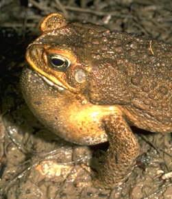
Repeated MeasuresIn an honours thesis from (1992), Mullens was investigating the ways that cane toads ( Bufo marinus ) respond to conditions of hypoxia. Toads show two different kinds of breathing patterns, lung or buccal, requiring them to be treated separately in the experiment. Her aim was to expose toads to a range of O2 concentrations, and record their breathing patterns, including parameters such as the expired volume for individual breaths. It was desirable to have around 8 replicates to compare the responses of the two breathing types, and the complication is that animals are expensive, and different individuals are likely to have different O2 profiles (leading to possibly reduced power). There are two main design options for this experiment;
- One animal per O2 treatment, 8 concentrations, 2 breathing types. With 8 replicates the experiment would require 128 animals, but that this could be analysed as a completely randomized design
- One O2 profile per animal, so that each animal would be used 8 times and only 16 animals are required (8 lung and 8 buccal breathers)
| Format of mullens.csv data file | |||||||||||||||||||||||||||||||||||||||||
|---|---|---|---|---|---|---|---|---|---|---|---|---|---|---|---|---|---|---|---|---|---|---|---|---|---|---|---|---|---|---|---|---|---|---|---|---|---|---|---|---|---|
|
 |
mullens <- read.table('../downloads/data/mullens.csv', header=T, sep=',', strip.white=T)
head(mullens)
  BREATH TOAD O2LEVEL FREQBUC SFREQBUC
1   lung    a       0    10.6    3.256
2   lung    a       5    18.8    4.336
3   lung    a      10    17.4    4.171
4   lung    a      15    16.6    4.074
5   lung    a      20     9.4    3.066
6   lung    a      30    11.4    3.376
mullens$nO2LEVEL <- mullens$O2LEVEL
mullens$O2LEVEL <- factor(mullens$O2LEVEL)
- What are the main hypotheses being tested?
- H0 Main Effect 1 (Factor A):
- H0 Main Effect 2 (Factor C):
- H0 Main Effect 3 (A*C):
- H0 Main Effect 1 (Factor A):
- We will now address all the assumptions.
Construct a boxplot to investigate the assumptions as they apply to the test of H0 Main Effect 1 (Factor A): This is done in two steps
- Construct a boxplot to investigate the assumptions as they apply to the test of H0 Main Effect 1 (Factor A):
Start by aggregating the data set by TOAD
(since the toads are the replicates for the between subject effect - BREATH) (HINT).
Then Construct a boxplot of aggregated mean FREQBUC against BREATH treatment
(HINT).
Any evidence of violations of the assumptions (y or n)?Show code
library(plyr)
mullens.ag <- ddply(mullens, ~BREATH + TOAD, function(df) data.frame(FREQBUC = mean(df$FREQBUC)))
boxplot(FREQBUC~BREATH, mullens.ag)
 Show ggplot code
library(plyr)
mullens.ag <- ddply(mullens, ~BREATH + TOAD, function(df) data.frame(FREQBUC = mean(df$FREQBUC)))
library(ggplot2)
ggplot(mullens.ag, aes(y=FREQBUC, x=BREATH)) + geom_boxplot()

Try a square-root transformation! - Construct a boxplot to investigate the assumptions as they apply to the test of H0 Main Effect 2 (Factor C): Since Factor C is tested against the overall residual in this case, this is a relatively straight forward procedure.(HINT).
Any evidence of violations of the assumptions (y or n)?
- Construct a boxplot to investigate the assumptions as they apply to the test of H0 the main interaction effect (A:C): Since A:C is tested against the overal residual, this is a relatively straight forward procedure.(HINT).
Any evidence of violations of the assumptions (y or n)?
- In addition to the above assumptions, the test of TOAD assumes that there is no TOAD by O2LEVEL interaction as this is the overal residual (the replicates).
That is, the test assumes that the effect of O2LEVEL is consistent in all TOADS.
Construct an interaction plot to examine whether there is any evidence of an interaction between TOAD and O2LEVEL
(HINT).
Any evidence of an interaction (y or n)?
- You must also check to see whether the proposed model
balanced.
Show codeIs it? (Yor N)
replications(SFREQBUC ~ BREATH + Error(TOAD) + O2LEVEL + BREATH:O2LEVEL,data=mullens)
$BREATH BREATH buccal lung 104 64 $O2LEVEL [1] 21 $`BREATH:O2LEVEL` O2LEVEL BREATH 0 5 10 15 20 30 40 50 buccal 13 13 13 13 13 13 13 13 lung 8 8 8 8 8 8 8 8!is.list(replications(SFREQBUC ~ BREATH + Error(TOAD) + O2LEVEL + BREATH:O2LEVEL,data=mullens))
[1] FALSE
- Finally, since the design is a repeated measures, there is a good chance that the assumption of
sphericity
has been violated balanced.
Show code
library(biology) epsi.GG.HF(aov(SFREQBUC ~ BREATH +O2LEVEL + BREATH:O2LEVEL+Error(TOAD),data=mullens))
$GG.eps [1] 0.4282 $HF.eps [1] 0.5173 $sigma [1] 0.7531
Show codeHas it (HINT)? (Y or N)library(nlme) acf(resid(lme(SFREQBUC~BREATH*O2LEVEL, random=~1|TOAD, data=mullens)))

Show codelibrary(plyr) mullens.ag <- ddply(mullens, ~BREATH + TOAD, function(df) data.frame(SFREQBUC = mean(sqrt(df$FREQBUC)))) boxplot(SFREQBUC~BREATH, mullens.ag)
 Show ggplot code
library(plyr)
mullens.ag <- ddply(mullens, ~BREATH + TOAD, function(df) data.frame(SFREQBUC = mean(sqrt(df$FREQBUC))))
library(ggplot2)
ggplot(mullens.ag, aes(y=SFREQBUC, x=BREATH)) + geom_boxplot()
 Show code
boxplot(SFREQBUC~O2LEVEL, mullens)
 Show ggplot code
ggplot(mullens, aes(y=SFREQBUC, x=O2LEVEL)) + geom_boxplot()
 Show code
boxplot(SFREQBUC~BREATH*O2LEVEL, mullens)
 Show ggplot code
ggplot(mullens, aes(y=SFREQBUC, x=O2LEVEL, color=BREATH)) + geom_boxplot()
 Show code
ggplot(mullens,aes(y=SFREQBUC, x=as.numeric(TOAD), color=O2LEVEL)) + geom_line(stat='summary', fun.y=mean)

with(mullens,interaction.plot(TOAD, O2LEVEL, SFREQBUC))

library(alr3)
tukey.nonadd.test(lm(SFREQBUC~TOAD+O2LEVEL, data=mullens))
    Test   Pvalue
3.079699 0.002072
- Construct a boxplot to investigate the assumptions as they apply to the test of H0 Main Effect 1 (Factor A):
Start by aggregating the data set by TOAD
(since the toads are the replicates for the between subject effect - BREATH) (HINT).
Then Construct a boxplot of aggregated mean FREQBUC against BREATH treatment
(HINT).
Any evidence of violations of the assumptions (y or n)?
- Assume that the assumption of compound symmetry/sphericity will be violated and perform a
split-plot ANOVA (repeated measures)
(HINT),
and complete the following table with corrected p-values (HINT).
- Fit a traditional linear model
Show code
# since the model is not balanced, cant use treatment contrasts
contrasts(mullens$BREATH) <- contr.sum
contrasts(mullens$O2LEVEL) <- contr.sum
mullens.aov <- aov(SFREQBUC ~ BREATH*O2LEVEL + Error(TOAD), data=mullens)
- Fit a range of linear mixed effects models (lme)
Show code
contrasts(mullens$BREATH) <- contr.treatment
contrasts(mullens$O2LEVEL) <- contr.treatment
library(nlme)
# random intercepts model
mullens.lme <- lme(SFREQBUC ~ BREATH*O2LEVEL, random=~1|TOAD, data=mullens, method='REML')

mullens.lme2 <- update(mullens.lme, correlation=corCompSymm(form=~1|TOAD))
mullens.lme3 <- update(mullens.lme, correlation=corAR1(form=~nO2LEVEL|TOAD))
AIC(mullens.lme,  mullens.lme2, mullens.lme3)
             df   AIC
mullens.lme  18 503.6
mullens.lme2 19 505.6
mullens.lme3 19 505.6
- Fit a range of linear mixed effects models (lmer)
Show code
library(lme4)
# random intercepts model
mullens.lmer <- lmer(SFREQBUC ~ BREATH*O2LEVEL+(1|TOAD), data=mullens, REML=TRUE)

mullens.lmer1 <- lmer(SFREQBUC ~ BREATH*O2LEVEL+(BREATH|TOAD), data=mullens, REML=TRUE,
   control=lmerControl(check.nobs.vs.nRE="ignore"))
AIC(mullens.lmer,  mullens.lmer1)
              df   AIC
mullens.lmer  18 503.6
mullens.lmer1 20 507.5
- Fit a traditional linear model
- Explore a range of model diagnostics
- Construct an
interaction plot
showing the density of worms against distance from Cu source, with each treatment as different lines (or different bars).
HINT
Show code
with(mullens, interaction.plot(O2LEVEL, BREATH, SFREQBUC))
 Show code
library(effects)
plot(allEffects(mullens.lme))

plot(allEffects(mullens.lme), multiline=TRUE)

- Residual plots
Show code
# Traditional ANOVA
par(mfrow=c(2,2))
plot(lm(mullens.aov))

# LME
plot(mullens.lme)

plot(residuals(mullens.lme, type='normalized') ~ fitted(mullens.lme))
plot(residuals(mullens.lme, type='normalized') ~ mullens$BREATH)
plot(residuals(mullens.lme, type='normalized') ~ mullens$O2LEVEL)
plot(residuals(mullens.lme, type='normalized') ~ interaction(mullens$BREATH,mullens$O2LEVEL))

#LMER
par(mfrow=c(1,1))
plot(mullens.lmer)

par(mfrow=c(2,2))
plot(resid(mullens.lmer) ~ mullens$BREATH)
plot(resid(mullens.lmer) ~ mullens$O2LEVEL)
plot(resid(mullens.lmer) ~ interaction(mullens$BREATH,mullens$O2LEVEL))

- Construct an
interaction plot
showing the density of worms against distance from Cu source, with each treatment as different lines (or different bars).
HINT
- Explore the model parameters
- Traditional
split-plot ANOVA (repeated measures)
(HINT),
and complete the following table with corrected p-values (HINT).
Source of variation df Mean Sq F-ratio P-value GG.P HF.P BREATH TOAD O2LEVEL BREATH:O2LEVEL Residuals Show codelibrary(biology) AnovaM(mullens.aov, RM=T, type="III")
   Sphericity Epsilon Values
-------------------------------
 Greenhouse.Geisser Huynh.Feldt
             0.4282      0.5173
Anova Table (Type III tests) Response: SFREQBUC Error: TOAD Df Sum Sq Mean Sq F value Pr(>F) BREATH 1 39.9 39.9 5.76 0.027 * Residuals 19 131.6 6.9 --- Signif. codes: 0 '***' 0.001 '**' 0.01 '*' 0.05 '.' 0.1 ' ' 1 Error: Within Df Sum Sq Mean Sq F value Pr(>F) O2LEVEL 7 75.4 10.78 14.3 9.0e-14 *** BREATH:O2LEVEL 7 56.4 8.05 10.7 1.2e-10 *** Residuals 133 100.2 0.75 --- Signif. codes: 0 '***' 0.001 '**' 0.01 '*' 0.05 '.' 0.1 ' ' 1 Greenhouse-Geisser corrected ANOVA table Response: SFREQBUC Error: TOAD Df Sum Sq Mean Sq F value Pr(>F) BREATH 0.428 39.9 39.9 5.76 0.048 * Residuals 19.000 131.6 6.9 --- Signif. codes: 0 '***' 0.001 '**' 0.01 '*' 0.05 '.' 0.1 ' ' 1 Error: Within Df Sum Sq Mean Sq F value Pr(>F) O2LEVEL 3 75.4 10.78 14.3 3.9e-08 *** BREATH:O2LEVEL 3 56.4 8.05 10.7 2.4e-06 *** Residuals 133 100.2 0.75 --- Signif. codes: 0 '***' 0.001 '**' 0.01 '*' 0.05 '.' 0.1 ' ' 1 Huynh-Feldt corrected ANOVA table Response: SFREQBUC Error: TOAD Df Sum Sq Mean Sq F value Pr(>F) BREATH 0.517 39.9 39.9 5.76 0.044 * Residuals 19.000 131.6 6.9 --- Signif. codes: 0 '***' 0.001 '**' 0.01 '*' 0.05 '.' 0.1 ' ' 1 Error: Within Df Sum Sq Mean Sq F value Pr(>F) O2LEVEL 3.62 75.4 10.78 14.3 3.8e-09 *** BREATH:O2LEVEL 3.62 56.4 8.05 10.7 4.2e-07 *** Residuals 133.00 100.2 0.75 --- Signif. codes: 0 '***' 0.001 '**' 0.01 '*' 0.05 '.' 0.1 ' ' 1 - LME
- LMER
Show codesummary(mullens.lme)
Linear mixed-effects model fit by REML Data: mullens AIC BIC logLik 503.6 558 -233.8 Random effects: Formula: ~1 | TOAD (Intercept) Residual StdDev: 0.8786 0.8678 Fixed effects: SFREQBUC ~ BREATH * O2LEVEL Value Std.Error DF t-value p-value (Intercept) 4.941 0.3425 133 14.426 0.0000 BREATH2 -3.391 0.5549 19 -6.112 0.0000 O2LEVEL2 -0.217 0.3404 133 -0.639 0.5242 O2LEVEL3 -0.548 0.3404 133 -1.609 0.1100 O2LEVEL4 -0.869 0.3404 133 -2.552 0.0118 O2LEVEL5 -1.544 0.3404 133 -4.537 0.0000 O2LEVEL6 -1.464 0.3404 133 -4.302 0.0000 O2LEVEL7 -2.246 0.3404 133 -6.597 0.0000 O2LEVEL8 -2.460 0.3404 133 -7.227 0.0000 BREATH2:O2LEVEL2 1.036 0.5515 133 1.879 0.0624 BREATH2:O2LEVEL3 2.333 0.5515 133 4.230 0.0000 BREATH2:O2LEVEL4 2.373 0.5515 133 4.303 0.0000 BREATH2:O2LEVEL5 3.298 0.5515 133 5.981 0.0000 BREATH2:O2LEVEL6 2.977 0.5515 133 5.398 0.0000 BREATH2:O2LEVEL7 3.617 0.5515 133 6.558 0.0000 BREATH2:O2LEVEL8 3.467 0.5515 133 6.286 0.0000 Correlation: (Intr) BREATH2 O2LEVEL2 O2LEVEL3 O2LEVEL4 O2LEVEL5 O2LEVEL6 O2LEVEL7 O2LEVEL8 BREATH2 -0.617 O2LEVEL2 -0.497 0.307 O2LEVEL3 -0.497 0.307 0.500 O2LEVEL4 -0.497 0.307 0.500 0.500 O2LEVEL5 -0.497 0.307 0.500 0.500 0.500 O2LEVEL6 -0.497 0.307 0.500 0.500 0.500 0.500 O2LEVEL7 -0.497 0.307 0.500 0.500 0.500 0.500 0.500 O2LEVEL8 -0.497 0.307 0.500 0.500 0.500 0.500 0.500 0.500 BREATH2:O2LEVEL2 0.307 -0.497 -0.617 -0.309 -0.309 -0.309 -0.309 -0.309 -0.309 BREATH2:O2LEVEL3 0.307 -0.497 -0.309 -0.617 -0.309 -0.309 -0.309 -0.309 -0.309 BREATH2:O2LEVEL4 0.307 -0.497 -0.309 -0.309 -0.617 -0.309 -0.309 -0.309 -0.309 BREATH2:O2LEVEL5 0.307 -0.497 -0.309 -0.309 -0.309 -0.617 -0.309 -0.309 -0.309 BREATH2:O2LEVEL6 0.307 -0.497 -0.309 -0.309 -0.309 -0.309 -0.617 -0.309 -0.309 BREATH2:O2LEVEL7 0.307 -0.497 -0.309 -0.309 -0.309 -0.309 -0.309 -0.617 -0.309 BREATH2:O2LEVEL8 0.307 -0.497 -0.309 -0.309 -0.309 -0.309 -0.309 -0.309 -0.617 BREATH2:O2LEVEL2 BREATH2:O2LEVEL3 BREATH2:O2LEVEL4 BREATH2:O2LEVEL5 BREATH2 O2LEVEL2 O2LEVEL3 O2LEVEL4 O2LEVEL5 O2LEVEL6 O2LEVEL7 O2LEVEL8 BREATH2:O2LEVEL2 BREATH2:O2LEVEL3 0.500 BREATH2:O2LEVEL4 0.500 0.500 BREATH2:O2LEVEL5 0.500 0.500 0.500 BREATH2:O2LEVEL6 0.500 0.500 0.500 0.500 BREATH2:O2LEVEL7 0.500 0.500 0.500 0.500 BREATH2:O2LEVEL8 0.500 0.500 0.500 0.500 BREATH2:O2LEVEL6 BREATH2:O2LEVEL7 BREATH2 O2LEVEL2 O2LEVEL3 O2LEVEL4 O2LEVEL5 O2LEVEL6 O2LEVEL7 O2LEVEL8 BREATH2:O2LEVEL2 BREATH2:O2LEVEL3 BREATH2:O2LEVEL4 BREATH2:O2LEVEL5 BREATH2:O2LEVEL6 BREATH2:O2LEVEL7 0.500 BREATH2:O2LEVEL8 0.500 0.500 Standardized Within-Group Residuals: Min Q1 Med Q3 Max -3.254224 -0.498850 0.008542 0.487520 3.231864 Number of Observations: 168 Number of Groups: 21intervals(mullens.lme)
Approximate 95% confidence intervals

 Fixed effects:
                    lower    est.   upper
(Intercept)       4.26353  4.9410  5.6184
BREATH2          -4.55287 -3.3914 -2.2300
O2LEVEL2         -0.89067 -0.2174  0.4559
O2LEVEL3         -1.22088 -0.5476  0.1257
O2LEVEL4         -1.54201 -0.8687 -0.1954
O2LEVEL5         -2.21768 -1.5444 -0.8711
O2LEVEL6         -2.13768 -1.4644 -0.7911
O2LEVEL7         -2.91895 -2.2457 -1.5724
O2LEVEL8         -3.13331 -2.4600 -1.7867
BREATH2:O2LEVEL2 -0.05462  1.0362  2.1271
BREATH2:O2LEVEL3  1.24190  2.3327  3.4236
BREATH2:O2LEVEL4  1.28209  2.3729  3.4638
BREATH2:O2LEVEL5  2.20762  3.2985  4.3893
BREATH2:O2LEVEL6  1.88588  2.9767  4.0676
BREATH2:O2LEVEL7  2.52600  3.6168  4.7077
BREATH2:O2LEVEL8  2.37608  3.4669  4.5578
attr(,"label")
[1] "Fixed effects:"

 Random Effects:
  Level: TOAD
                 lower   est. upper
sd((Intercept)) 0.6143 0.8786 1.256

 Within-group standard error:
 lower   est.  upper
0.7696 0.8678 0.9786
## If we need an ANOVA table, we must remember that as the design is unbalanced ## Type III Sums-of-Squares must be used (and thus not treatment contrasts). anova(update(mullens.lme, contrasts=list(BREATH='contr.sum',O2LEVEL='contr.sum')), type='marginal')
               numDF denDF F-value p-value
(Intercept)        1   133  244.68  <.0001
BREATH             1    19    5.76  0.0268
O2LEVEL            7   133    4.88  0.0001
BREATH:O2LEVEL     7   133   10.69  <.0001
Show codelibrary(lmerTest) mullens.lmer <- lmer(SFREQBUC ~ BREATH*O2LEVEL+(1|TOAD), data=mullens, REML=TRUE) #mullens.lmer1 <- update(mullens.lmer) summary(mullens.lmer)
Linear mixed model fit by REML t-tests use Satterthwaite approximations to degrees of freedom [ merModLmerTest] Formula: SFREQBUC ~ BREATH * O2LEVEL + (1 | TOAD) Data: mullens REML criterion at convergence: 467.6 Scaled residuals: Min 1Q Median 3Q Max -3.254 -0.499 0.009 0.488 3.232 Random effects: Groups Name Variance Std.Dev. TOAD (Intercept) 0.772 0.879 Residual 0.753 0.868 Number of obs: 168, groups: TOAD, 21 Fixed effects: Estimate Std. Error df t value Pr(>|t|) (Intercept) 4.941 0.343 54.400 14.43 < 2e-16 *** BREATH2 -3.391 0.555 54.400 -6.11 1.1e-07 *** O2LEVEL2 -0.217 0.340 133.000 -0.64 0.524 O2LEVEL3 -0.548 0.340 133.000 -1.61 0.110 O2LEVEL4 -0.869 0.340 133.000 -2.55 0.012 * O2LEVEL5 -1.544 0.340 133.000 -4.54 1.3e-05 *** O2LEVEL6 -1.464 0.340 133.000 -4.30 3.3e-05 *** O2LEVEL7 -2.246 0.340 133.000 -6.60 9.1e-10 *** O2LEVEL8 -2.460 0.340 133.000 -7.23 3.5e-11 *** BREATH2:O2LEVEL2 1.036 0.551 133.000 1.88 0.062 . BREATH2:O2LEVEL3 2.333 0.551 133.000 4.23 4.3e-05 *** BREATH2:O2LEVEL4 2.373 0.551 133.000 4.30 3.2e-05 *** BREATH2:O2LEVEL5 3.298 0.551 133.000 5.98 1.9e-08 *** BREATH2:O2LEVEL6 2.977 0.551 133.000 5.40 3.0e-07 *** BREATH2:O2LEVEL7 3.617 0.551 133.000 6.56 1.1e-09 *** BREATH2:O2LEVEL8 3.467 0.551 133.000 6.29 4.3e-09 *** --- Signif. codes: 0 '***' 0.001 '**' 0.01 '*' 0.05 '.' 0.1 ' ' 1 Correlation of Fixed Effects: (Intr) BREATH2 O2LEVEL2 O2LEVEL3 O2LEVEL4 O2LEVEL5 O2LEVEL6 O2LEVEL7 O2LEVEL8 BREATH2 -0.617 O2LEVEL2 -0.497 0.307 O2LEVEL3 -0.497 0.307 0.500 O2LEVEL4 -0.497 0.307 0.500 0.500 O2LEVEL5 -0.497 0.307 0.500 0.500 0.500 O2LEVEL6 -0.497 0.307 0.500 0.500 0.500 0.500 O2LEVEL7 -0.497 0.307 0.500 0.500 0.500 0.500 0.500 O2LEVEL8 -0.497 0.307 0.500 0.500 0.500 0.500 0.500 0.500 BREATH2:O2LEVEL2 0.307 -0.497 -0.617 -0.309 -0.309 -0.309 -0.309 -0.309 -0.309 BREATH2:O2LEVEL3 0.307 -0.497 -0.309 -0.617 -0.309 -0.309 -0.309 -0.309 -0.309 BREATH2:O2LEVEL4 0.307 -0.497 -0.309 -0.309 -0.617 -0.309 -0.309 -0.309 -0.309 BREATH2:O2LEVEL5 0.307 -0.497 -0.309 -0.309 -0.309 -0.617 -0.309 -0.309 -0.309 BREATH2:O2LEVEL6 0.307 -0.497 -0.309 -0.309 -0.309 -0.309 -0.617 -0.309 -0.309 BREATH2:O2LEVEL7 0.307 -0.497 -0.309 -0.309 -0.309 -0.309 -0.309 -0.617 -0.309 BREATH2:O2LEVEL8 0.307 -0.497 -0.309 -0.309 -0.309 -0.309 -0.309 -0.309 -0.617 BREATH2:O2LEVEL2 BREATH2:O2LEVEL3 BREATH2:O2LEVEL4 BREATH2:O2LEVEL5 BREATH2 O2LEVEL2 O2LEVEL3 O2LEVEL4 O2LEVEL5 O2LEVEL6 O2LEVEL7 O2LEVEL8 BREATH2:O2LEVEL2 BREATH2:O2LEVEL3 0.500 BREATH2:O2LEVEL4 0.500 0.500 BREATH2:O2LEVEL5 0.500 0.500 0.500 BREATH2:O2LEVEL6 0.500 0.500 0.500 0.500 BREATH2:O2LEVEL7 0.500 0.500 0.500 0.500 BREATH2:O2LEVEL8 0.500 0.500 0.500 0.500 BREATH2:O2LEVEL6 BREATH2:O2LEVEL7 BREATH2 O2LEVEL2 O2LEVEL3 O2LEVEL4 O2LEVEL5 O2LEVEL6 O2LEVEL7 O2LEVEL8 BREATH2:O2LEVEL2 BREATH2:O2LEVEL3 BREATH2:O2LEVEL4 BREATH2:O2LEVEL5 BREATH2:O2LEVEL6 BREATH2:O2LEVEL7 0.500 BREATH2:O2LEVEL8 0.500 0.500anova(mullens.lmer, ddf='Satterthwaite')
Analysis of Variance Table of type 3 with Satterthwaite approximation for degrees of freedom Sum Sq Mean Sq NumDF DenDF F.value Pr(>F) BREATH 4.3 4.34 1 19 5.76 0.027 * O2LEVEL 25.7 3.68 7 133 4.88 6.3e-05 *** BREATH:O2LEVEL 56.4 8.05 7 133 10.69 1.2e-10 *** --- Signif. codes: 0 '***' 0.001 '**' 0.01 '*' 0.05 '.' 0.1 ' ' 1anova(mullens.lmer, ddf='Kenward-Roger')
Analysis of Variance Table of type 3  with  Kenward-Roger
approximation for degrees of freedom
               Sum Sq Mean Sq NumDF DenDF F.value  Pr(>F)
BREATH            4.3    4.34     1    19    5.76   0.027 *
O2LEVEL          25.7    3.68     7   133    4.88 6.3e-05 ***
BREATH:O2LEVEL   56.4    8.05     7   133   10.69 1.2e-10 ***
---
Signif. codes:  0 '***' 0.001 '**' 0.01 '*' 0.05 '.' 0.1 ' ' 1
- Traditional
split-plot ANOVA (repeated measures)
(HINT),
and complete the following table with corrected p-values (HINT).
- In order to tease out the interaction, we could analyse the effects of the main factor (COPPER) separately for each Distance and/or investigate the effects of Distance separately for each of the three copper treatments.
Recall that when performing such simple main effects, it is necessary to use the residual terms from the global analyses as these are likely to be better estimates (as they are based on a larger amount of data).
- Investigate the effects of copper separately for each of the
four distances HINT
- Traditional ANOVA
Show code
AnovaM(mainEffects(mullens.aov, at=BREATH=='buccal'),type='III')
Error: TOAD Df Sum Sq Mean Sq F value Pr(>F) INT 1 39.9 39.9 5.76 0.027 * Residuals 19 131.6 6.9 --- Signif. codes: 0 '***' 0.001 '**' 0.01 '*' 0.05 '.' 0.1 ' ' 1 Error: Within Df Sum Sq Mean Sq F value Pr(>F) INT 7 19.9 2.84 3.78 0.00091 *** O2LEVEL 7 75.4 10.78 14.31 9e-14 *** Residuals 133 100.2 0.75 --- Signif. codes: 0 '***' 0.001 '**' 0.01 '*' 0.05 '.' 0.1 ' ' 1AnovaM(mainEffects(mullens.aov, at=BREATH=='lung'),type='III')
Error: TOAD Df Sum Sq Mean Sq F value Pr(>F) INT 1 39.9 39.9 5.76 0.027 * Residuals 19 131.6 6.9 --- Signif. codes: 0 '***' 0.001 '**' 0.01 '*' 0.05 '.' 0.1 ' ' 1 Error: Within Df Sum Sq Mean Sq F value Pr(>F) INT 7 75.4 10.78 14.31 9e-14 *** O2LEVEL 7 19.9 2.84 3.78 0.00091 *** Residuals 133 100.2 0.75 --- Signif. codes: 0 '***' 0.001 '**' 0.01 '*' 0.05 '.' 0.1 ' ' 1 - LME
Show code
mullens<-within(mullens,{O2LEVEL2=ifelse(BREATH=='buccal', '1',as.character(O2LEVEL))})
mullens<-within(mullens,{BO=interaction(O2LEVEL2,BREATH)})
anova(update(mullens.lme, ~BO + . - BREATH - BREATH:O2LEVEL), type='marginal')
            numDF denDF F-value p-value
(Intercept)     1   132  208.11  <.0001
BO              8   132   10.08  <.0001
O2LEVEL         7   132   14.31  <.0001
mullens<-within(mullens,{O2LEVEL2=ifelse(BREATH=='lung', '1',as.character(O2LEVEL))})
mullens<-within(mullens,{BO=interaction(O2LEVEL2,BREATH)})
anova(update(mullens.lme, ~BO + . - BREATH - BREATH:O2LEVEL), type='marginal')
            numDF denDF F-value p-value
(Intercept)     1   132  208.11  <.0001
BO              8   132   10.08  <.0001
O2LEVEL         7   132    3.78   9e-04
- LMER
Show code
library(lmerTest)
mullens<-within(mullens,{O2LEVEL2=ifelse(BREATH=='buccal', '1',as.character(O2LEVEL))})
mullens<-within(mullens,{BO=interaction(O2LEVEL2,BREATH)})
mullens.lmer <- lmer(SFREQBUC ~ O2LEVEL+BO+(1|TOAD), data=mullens, REML=TRUE)
anova(mullens.lmer, ddf='Kenward-Roger')
Analysis of Variance Table of type 3 with Kenward-Roger approximation for degrees of freedom Sum Sq Mean Sq NumDF DenDF F.value Pr(>F) O2LEVEL 75.4 10.78 7 133 14.31 9.0e-14 *** BO 60.1 7.51 8 123 9.97 1.2e-10 *** --- Signif. codes: 0 '***' 0.001 '**' 0.01 '*' 0.05 '.' 0.1 ' ' 1mullens<-within(mullens,{O2LEVEL2=ifelse(BREATH=='lung', '1',as.character(O2LEVEL))}) mullens<-within(mullens,{BO=interaction(O2LEVEL2,BREATH)}) mullens.lmer <- lmer(SFREQBUC ~ O2LEVEL+BO+(1|TOAD), data=mullens, REML=TRUE) anova(mullens.lmer, ddf='Kenward-Roger')
Analysis of Variance Table of type 3  with  Kenward-Roger
approximation for degrees of freedom
        Sum Sq Mean Sq NumDF DenDF F.value  Pr(>F)
O2LEVEL   19.9    2.84     7   133    3.78 0.00091 ***
BO        60.1    7.51     8   123    9.97 1.2e-10 ***
---
Signif. codes:  0 '***' 0.001 '**' 0.01 '*' 0.05 '.' 0.1 ' ' 1
What conclusions would you draw from these four analyses?
- Traditional ANOVA
-
Examine the variance components
- LME
Show code
VarCorr(mullens.lme)
TOAD = pdLogChol(1) Variance StdDev (Intercept) 0.7719 0.8786 Residual 0.7531 0.8678 - LMER
Show code
print(VarCorr(mullens.lmer), comp=c('Variance','Std.Dev.'))
 Groups   Name        Variance Std.Dev.
 TOAD     (Intercept) 0.772    0.879
 Residual             0.753    0.868
as.data.frame(VarCorr(mullens.lmer))
       grp        var1 var2   vcov  sdcor
1     TOAD (Intercept)  0.7719 0.8786
2 Residual          0.7531 0.8678
- LME
- Finally, a summary figure would be nice...
- LME
Show code
coefs <- fixef(mullens.lme)
newdata <- with(mullens, expand.grid(BREATH=levels(BREATH), O2LEVEL=levels(O2LEVEL)))
Xmat <- model.matrix(~BREATH*O2LEVEL, newdata)
pred <- as.vector(coefs %*% t(Xmat) )
se <- sqrt(diag(Xmat %*% vcov(mullens.lme) %*% t(Xmat)))
sigma <- mullens.lme$sigma
newdata$fit <- (pred)^2
newdata$lower <- (pred - 2*se)^2
newdata$upper <- (pred + 2*se)^2
newdata$plower <- (pred - 2*(se+sigma))^2
newdata$pupper <- (pred + 2*(se+sigma))^2

library(ggplot2)
ggplot(newdata, aes(y=fit, x=as.numeric(as.character(O2LEVEL)), fill=BREATH)) +
  geom_line(aes(linetype=BREATH)) +
  #geom_line()+
  geom_linerange(aes(ymin=lower, ymax=upper), show_guide=FALSE)+
  geom_point(size=3, shape=21)+
  scale_y_continuous(expression(Frequency~of~buccal~breathing))+
  scale_x_continuous('Oxygen concentration (%)')+
  scale_fill_manual('Breathing type', breaks=c('buccal','lung'), values=c('black','white'),
                    labels=c('Buccal','Lung'))+
  scale_linetype_manual('Breathing type', breaks=c('buccal','lung'), values=c('solid','dashed'),
                    labels=c('Buccal','Lung'))+
  theme_classic() +
  theme(legend.justification=c(1,1), legend.position=c(1,1),
        legend.key.width=unit(3,'lines'),
        axis.title.y=element_text(vjust=2, size=rel(1.2)),
        axis.title.x=element_text(vjust=-1, size=rel(1.2)),
        plot.margin=unit(c(0.5,0.5,1,2),'lines'))

- LMER
Show code
coefs <- fixef(mullens.lme)
newdata <- with(mullens, expand.grid(BREATH=levels(BREATH), O2LEVEL=levels(O2LEVEL)))
Xmat <- model.matrix(~BREATH*O2LEVEL, newdata)
pred <- as.vector(coefs %*% t(Xmat) )
se <- sqrt(diag(Xmat %*% vcov(mullens.lme) %*% t(Xmat)))
sigma <- VarCorr(mullens.lmer)$TOAD[1]
newdata$fit <- (pred)^2
newdata$lower <- (pred - 2*se)^2
newdata$upper <- (pred + 2*se)^2
newdata$plower <- (pred - 2*(se+sigma))^2
newdata$pupper <- (pred + 2*(se+sigma))^2

library(ggplot2)
ggplot(newdata, aes(y=fit, x=as.numeric(as.character(O2LEVEL)), fill=BREATH)) +
  geom_line(aes(linetype=BREATH)) +
  #geom_line()+
  geom_linerange(aes(ymin=lower, ymax=upper), show_guide=FALSE)+
  geom_point(size=3, shape=21)+
  scale_y_continuous(expression(Frequency~of~buccal~breathing))+
  scale_x_continuous('Oxygen concentration (%)')+
  scale_fill_manual('Breathing type', breaks=c('buccal','lung'), values=c('black','white'),
                    labels=c('Buccal','Lung'))+
  scale_linetype_manual('Breathing type', breaks=c('buccal','lung'), values=c('solid','dashed'),
                    labels=c('Buccal','Lung'))+
  theme_classic() +
  theme(legend.justification=c(1,1), legend.position=c(1,1),
        legend.key.width=unit(3,'lines'),
        axis.title.y=element_text(vjust=2, size=rel(1.2)),
        axis.title.x=element_text(vjust=-1, size=rel(1.2)),
        plot.margin=unit(c(0.5,0.5,1,2),'lines'))

- LME
- Of course as an alternative to modelling oxygen concentration as a categorical variable, we could alternatively model it as a numeric covariate (with polynomial terms to model the non-linearity).
Show code# fit random intercepts models with and without AR1 with O2 level as a numeric covariate mullens.lme1 <- lme(SFREQBUC~BREATH*nO2LEVEL, random=~1|TOAD,data=mullens) mullens.lme2 <- update(mullens.lme1, correlation=corAR1(form=~nO2LEVEL|TOAD)) anova(mullens.lme1, mullens.lme2)
             Model df   AIC   BIC logLik   Test   L.Ratio p-value
mullens.lme1     1  6 517.7 536.3 -252.9
mullens.lme2     2  7 519.7 541.4 -252.9 1 vs 2 1.137e-13       1
# Retain simpler model

summary(mullens.lme1)
Linear mixed-effects model fit by REML
 Data: mullens
    AIC   BIC logLik
  517.7 536.3 -252.9

Random effects:
 Formula: ~1 | TOAD
        (Intercept) Residual
StdDev:      0.8724   0.9166

Fixed effects: SFREQBUC ~ BREATH * nO2LEVEL
                  Value Std.Error  DF t-value p-value
(Intercept)       4.852    0.2833 145  17.126   0e+00
BREATH2          -2.311    0.4590  19  -5.035   1e-04
nO2LEVEL         -0.051    0.0055 145  -9.239   0e+00
BREATH2:nO2LEVEL  0.062    0.0089 145   6.906   0e+00
 Correlation:
                 (Intr) BREATH2 nO2LEV
BREATH2          -0.617
nO2LEVEL         -0.412  0.255
BREATH2:nO2LEVEL  0.255 -0.412  -0.617

Standardized Within-Group Residuals:
     Min       Q1      Med       Q3      Max
-4.14300 -0.48581  0.08982  0.46410  3.02620

Number of Observations: 168
Number of Groups: 21
# For fitting the initial global candidate models, define sum contrasts (if want to produce an ANOVA table) anova(update(mullens.lme1, contrasts=list(BREATH='contr.sum')), type='marginal')
                numDF denDF F-value p-value
(Intercept)         1   145  259.39  <.0001
BREATH              1    19   25.35   1e-04
nO2LEVEL            1   145   20.25  <.0001
BREATH:nO2LEVEL     1   145   47.69  <.0001
## There is evidence  of an interaction, so split up by breathing type via contrasts.

## Compare (contrast) main effects of 02 level using Wald Chi-square statistic.
library(car)
# Slope when BREATH='buccal'
linearHypothesis(mullens.lme1, 'nO2LEVEL=0')
Linear hypothesis test

Hypothesis:
nO2LEVEL = 0

Model 1: restricted model
Model 2: SFREQBUC ~ BREATH * nO2LEVEL

  Df Chisq Pr(>Chisq)
1
2  1  85.4     <2e-16 ***
---
Signif. codes:  0 '***' 0.001 '**' 0.01 '*' 0.05 '.' 0.1 ' ' 1
# Slope when BREATH='lung'
linearHypothesis(mullens.lme1, 'nO2LEVEL+BREATH2:nO2LEVEL=0')
Linear hypothesis test

Hypothesis:
nO2LEVEL  + BREATH2:nO2LEVEL = 0

Model 1: restricted model
Model 2: SFREQBUC ~ BREATH * nO2LEVEL

  Df Chisq Pr(>Chisq)
1
2  1  2.34       0.13
#OR alternatively, we could use the phia package
library(phia)
testInteractions(mullens.lme1, fixed="BREATH", slope="nO2LEVEL")
Adjusted slope for nO2LEVEL Chisq Test: P-value adjustment method: holm Value Df Chisq Pr(>Chisq) buccal -0.0508 1 85.36 <2e-16 *** lung 0.0107 1 2.34 0.13 --- Signif. codes: 0 '***' 0.001 '**' 0.01 '*' 0.05 '.' 0.1 ' ' 1testFactors(mullens.lme1, levels=list(BREATH=c('buccal')), terms.formula = ~0+nO2LEVEL)
Call: knit(model = "ws9.4a_knit_.html", levels = "ws9.4a.html") Term nO2LEVEL Adjusted slope for nO2LEVEL: -0.0508 Linear hypothesis test Hypothesis: nO2LEVEL = 0 Model 1: restricted model Model 2: SFREQBUC ~ BREATH * nO2LEVEL Df Chisq Pr(>Chisq) 1 2 1 85.36 <2e-16 *** --- Signif. codes: 0 '***' 0.001 '**' 0.01 '*' 0.05 '.' 0.1 ' ' 1 ------testFactors(mullens.lme1, levels=list(BREATH=c('lung')), terms.formula = ~0+nO2LEVEL)
Call: knit(model = "ws9.4a_knit_.html", levels = "ws9.4a.html")

Term nO2LEVEL

Adjusted slope for nO2LEVEL:

0.01072

Linear hypothesis test

Hypothesis:
nO2LEVEL  + BREATH2:nO2LEVEL = 0

Model 1: restricted model
Model 2: SFREQBUC ~ BREATH * nO2LEVEL

  Df Chisq Pr(>Chisq)
1
2  1 2.338      0.126
------
## Now lets make it a little more interesting by modelling a polynomial term for O2 level mullens.lme1 <- lme(SFREQBUC~BREATH*poly(nO2LEVEL,2), random=~1|TOAD,data=mullens) mullens.lme2 <- update(mullens.lme1,correlation=corAR1(form=~nO2LEVEL|TOAD)) anova(mullens.lme1, mullens.lme2)
             Model df   AIC   BIC logLik   Test L.Ratio p-value
mullens.lme1     1  8 477.5 502.2 -230.8
mullens.lme2     2  9 479.5 507.3 -230.8 1 vs 2       0       1
summary(mullens.lme1)
Linear mixed-effects model fit by REML Data: mullens AIC BIC logLik 477.5 502.2 -230.8 Random effects: Formula: ~1 | TOAD (Intercept) Residual StdDev: 0.8787 0.8667 Fixed effects: SFREQBUC ~ BREATH * poly(nO2LEVEL, 2) Value Std.Error DF t-value p-value (Intercept) 3.772 0.2581 143 14.616 0.0000 BREATH2 -1.004 0.4182 19 -2.400 0.0268 poly(nO2LEVEL, 2)1 -10.764 1.1015 143 -9.771 0.0000 poly(nO2LEVEL, 2)2 1.311 1.1015 143 1.190 0.2360 BREATH2:poly(nO2LEVEL, 2)1 13.034 1.7847 143 7.303 0.0000 BREATH2:poly(nO2LEVEL, 2)2 -7.229 1.7847 143 -4.051 0.0001 Correlation: (Intr) BREATH p(O2LEVEL,2)1 p(O2LEVEL,2)2 BREATH2:(O2LEVEL,2)1 BREATH2 -0.617 poly(nO2LEVEL, 2)1 0.000 0.000 poly(nO2LEVEL, 2)2 0.000 0.000 0.000 BREATH2:poly(nO2LEVEL, 2)1 0.000 0.000 -0.617 0.000 BREATH2:poly(nO2LEVEL, 2)2 0.000 0.000 0.000 -0.617 0.000 Standardized Within-Group Residuals: Min Q1 Med Q3 Max -3.62595 -0.54018 0.02722 0.45335 3.06139 Number of Observations: 168 Number of Groups: 21anova(update(mullens.lme1, contrasts=list(BREATH='contr.sum')), type='marginal')
                         numDF denDF F-value p-value
(Intercept)                  1   143  244.68  <.0001
BREATH                       1    19    5.76  0.0268
poly(nO2LEVEL, 2)            2   143   14.66  <.0001
BREATH:poly(nO2LEVEL, 2)     2   143   34.87  <.0001
## Conclusion: not surprisingly, there is an interaction.

# test of linear trend when BREATH='buccal'
linearHypothesis(mullens.lme1, 'poly(nO2LEVEL, 2)1=0')
Linear hypothesis test

Hypothesis:
poly(nO2LEVEL, 2)1 = 0

Model 1: restricted model
Model 2: SFREQBUC ~ BREATH * poly(nO2LEVEL, 2)

  Df Chisq Pr(>Chisq)
1
2  1  95.5     <2e-16 ***
---
Signif. codes:  0 '***' 0.001 '**' 0.01 '*' 0.05 '.' 0.1 ' ' 1
# test of quadratic trend when BREATH='buccal'
linearHypothesis(mullens.lme1, 'poly(nO2LEVEL, 2)2=0')
Linear hypothesis test

Hypothesis:
poly(nO2LEVEL, 2)2 = 0

Model 1: restricted model
Model 2: SFREQBUC ~ BREATH * poly(nO2LEVEL, 2)

  Df Chisq Pr(>Chisq)
1
2  1  1.42       0.23
# test of linear trend when BREATH='lung'
linearHypothesis(mullens.lme1, 'poly(nO2LEVEL, 2)1+BREATH2:poly(nO2LEVEL, 2)1=0')
Linear hypothesis test

Hypothesis:
poly(nO2LEVEL, 2)1  + BREATH2:poly(nO2LEVEL, 2)1 = 0

Model 1: restricted model
Model 2: SFREQBUC ~ BREATH * poly(nO2LEVEL, 2)

  Df Chisq Pr(>Chisq)
1
2  1  2.61       0.11
# test of quadratic trend when BREATH='lung'
linearHypothesis(mullens.lme1, 'poly(nO2LEVEL, 2)2+BREATH2:poly(nO2LEVEL, 2)2=0')
Linear hypothesis test

Hypothesis:
poly(nO2LEVEL, 2)2  + BREATH2:poly(nO2LEVEL, 2)2 = 0

Model 1: restricted model
Model 2: SFREQBUC ~ BREATH * poly(nO2LEVEL, 2)

  Df Chisq Pr(>Chisq)
1
2  1  17.8    2.5e-05 ***
---
Signif. codes:  0 '***' 0.001 '**' 0.01 '*' 0.05 '.' 0.1 ' ' 1
## Conclusions:  whilst the rate of buccal breathing declines linearly with increasing O2 concentration
##               in buccal breathing toads, lung breathing toads show an initial increase to an optimum
##               before declining.
- Investigate the effects of copper separately for each of the
four distances HINT