Workshop 9.2b - Nested designs (hierarchical models)
28 Jan 2015
Nested ANOVA (Mixed effects) references
- McCarthy (2007) - Chpt ?
- Kery (2010) - Chpt ?
- Gelman & Hill (2007) - Chpt ?
- Logan (2010) - Chpt 12
- Quinn & Keough (2002) - Chpt 9
Nested ANOVA - one between factor
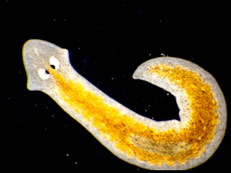
In an unusually detailed preparation for an Environmental Effects Statement for a proposed discharge of dairy wastes into the Curdies River, in western Victoria, a team of stream ecologists wanted to describe the basic patterns of variation in a stream invertebrate thought to be sensitive to nutrient enrichment. As an indicator species, they focused on a small flatworm, Dugesia, and started by sampling populations of this worm at a range of scales. They sampled in two seasons, representing different flow regimes of the river - Winter and Summer. Within each season, they sampled three randomly chosen (well, haphazardly, because sites are nearly always chosen to be close to road access) sites. A total of six sites in all were visited, 3 in each season. At each site, they sampled six stones, and counted the number of flatworms on each stone.
Download Curdies data set| Format of curdies.csv data files | |||||||||||||||||||||||||||||||||||||||||||||
|---|---|---|---|---|---|---|---|---|---|---|---|---|---|---|---|---|---|---|---|---|---|---|---|---|---|---|---|---|---|---|---|---|---|---|---|---|---|---|---|---|---|---|---|---|---|
|
 |
||||||||||||||||||||||||||||||||||||||||||||
The hierarchical nature of this design can be appreciated when we examine an illustration of the spatial and temporal scale of the measurements.
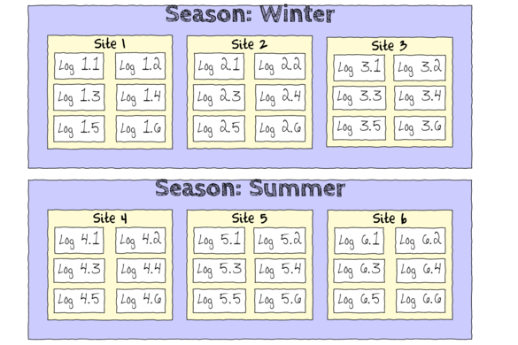
- Within each of the two Seasons, there were three separate Sites (Sites not repeatidly measured across Seasons).
- Within each of the Sites, six logs were selected (haphazardly) from which the number of flatworms were counted.
We construct the model in much the same way. That is:
- The observed number of flatworm per log (for a given Site) is equal to (modelled against) the mean number for that Site
plus a random amount drawn from a normal distribution with a mean of zero and a certain degree of variability (precision).
Number of flatwormlog i = βSite j,i + εi where ε ∼ N(0,σ2)
- The mean number of flatworm per Site (within a given Season) is equal to (modelled against) the mean number for that Season
plus a random amount drawn from a normal distribution with a means of zero and a certain degree of variability (precision).
μSite j = γSeason j + εj where ε ∼ N(0,σ2)
The SITE variable is conveniently already coded as a numeric series (starting at 1).
Open the curdies data file.curdies <- read.table('../downloads/data/curdies.csv', header=T, sep=',', strip.white=T) head(curdies)
  SEASON SITE DUGESIA S4DUGES
1 WINTER    1  0.6477  0.8971
2 WINTER    1  6.0962  1.5713
3 WINTER    1  1.3106  1.0700
4 WINTER    1  1.7253  1.1461
5 WINTER    1  1.4594  1.0991
6 WINTER    1  1.0576  1.0141
- Lets start by performing some exploratory data analysis to help us identify any issues with the data as
well as helping to try to identify a possible model to fit.
- Boxplots for the main effect (Season)
Show codeIs there any evidence of non-normality and/or heterogeneity (Y or N)
library(dplyr)
curdies.ag <- curdies %>% group_by(SEASON,SITE) %>% summarize(DUGESIA=mean(DUGESIA))
curdies.ag
Source: local data frame [6 x 3]
Groups: SEASON

  SEASON SITE DUGESIA
1 SUMMER    4  0.4191
2 SUMMER    5  0.2291
3 SUMMER    6  0.1942
4 WINTER    1  2.0494
5 WINTER    2  4.1819
6 WINTER    3  0.6782
#OR equivalently with the plyr package
library(plyr)
ddply(curdies, ~SEASON+SITE, numcolwise(mean))
  SEASON SITE DUGESIA S4DUGES
1 SUMMER    4  0.4191  0.3508
2 SUMMER    5  0.2291  0.1805
3 SUMMER    6  0.1942  0.3811
4 WINTER    1  2.0494  1.1329
5 WINTER    2  4.1819  1.2719
6 WINTER    3  0.6782  0.8679
detach(package:plyr) #since dplyr and plyr do not play nicely together

library(ggplot2)
ggplot(curdies.ag, aes(y=DUGESIA, x=SEASON)) + geom_boxplot()

If so, assess whether a transformation (such as a forth-root transformation) will address the violations and then make the appropriate corrections - Consider a transformation (such as forth-root transform) and redo boxplots for the main effect (Season)
Show codeDoes a forth-root transformation improve the data with respect to normality and homogeneity of variance (Y or N)?
curdies.ag <- curdies %>% group_by(SEASON,SITE) %>% summarize(DUGESIA=mean(DUGESIA^0.25))
curdies.ag
Source: local data frame [6 x 3]
Groups: SEASON

  SEASON SITE DUGESIA
1 SUMMER    4  0.3508
2 SUMMER    5  0.1805
3 SUMMER    6  0.3811
4 WINTER    1  1.1329
5 WINTER    2  1.2719
6 WINTER    3  0.8679
ggplot(curdies.ag, aes(y=DUGESIA, x=SEASON)) + geom_boxplot()

- Boxplots for the main effect (Season)
- Fit the hierarchical model.
Use with effects (or matrix) parameterization for the 'fixed effects' and means (or matrix) parameterization for the 'random effects'.
Note the following points:
- Non-informative priors for residual precision (standard deviations) should be defined as vague uniform distributions rather than gamma distributions. This prevents the chains from walking to close to parameter estimates of 0. Alternatively, Gelman recommends the use of weakly informative half-cauchy distributions for variances in hierarchical designs.
- Finite-population standard deviation for Site (the within group factor) should reflect standard deviation between Sites within season (not standard deviation between all Sites). Unfortunately, the BUGS language does not offer a mechanism to determine which indexes match certain criteria (for example which Sites correspond to which Season), nor does it allow variables to be redefined. One way to allow us to generate multiple standard deviations is to create an offset vector that can be used to indicate the range of Site numbers that are within which Season.
- As this is a multi-level design in which the Season 'replicates' are determined by the Site means, it is important that firstly, the number of levels of the within Group factor (Season) reflects this, and secondly that the factor levels of the within group factor (Season) correspond to the factor levels of the group factor (Site). In this case, the Sites are labeled 1-6, but the first three Sites are in Winter. R will naturally label Winter as the second level (as alphabetically W comes after S for summer). Thus without intervention or careful awareness, it will appear that the Winter means are higher than the Summer means, when it is actually the other way around. One way to check this, is create the data list and check that all the factor levels are listed in increasing numerical order.
View preparation codesites<-ddply(curdies, ~SITE, catcolwise(unique)) offset <- c(match(levels(sites$SEASON),sites$SEASON), length(sites$SEASON)+1) offset
[1] 4 1 7
curdies.list <- with(curdies,
   list(dugesia=DUGESIA,
        season=as.numeric(SEASON),
                site=as.numeric(SITE),
                n=nrow(curdies), nSeason=length(levels(as.factor(SEASON))),
                nSite=length(levels(as.factor(SITE))),
                SiteOffset=offset
                )
)
curdies.list
$dugesia
 [1]  0.6477  6.0962  1.3106  1.7253  1.4594  1.0576  1.0163 16.1968  1.1681  1.0243  2.0113  3.6746
[13]  0.6891  1.2191  1.1131  0.6569  0.1361  0.2547  0.0000  0.0000  0.9411  0.0000  0.0000  1.5735
[25]  1.3745  0.0000  0.0000  0.0000  0.0000  0.0000  0.0000  0.0000  0.1329  0.0000  0.6580  0.3745

$season
 [1] 2 2 2 2 2 2 2 2 2 2 2 2 2 2 2 2 2 2 1 1 1 1 1 1 1 1 1 1 1 1 1 1 1 1 1 1

$site
 [1] 1 1 1 1 1 1 2 2 2 2 2 2 3 3 3 3 3 3 4 4 4 4 4 4 5 5 5 5 5 5 6 6 6 6 6 6

$n
[1] 36

$nSeason
[1] 2

$nSite
[1] 6

$SiteOffset
[1] 4 1 7
## notice that The Season variable has as many entries as there were plots
## rather than having as many as there were Sites.
## Also notice that Winter is the second Season according to the factor levels
## Finally notice that the offset values are not in order

#season <- with(curdies,SEASON[match(unique(SITE),SITE)])
#season <- factor(season, levels=unique(season))

curdies$SEASON <- factor(curdies$SEASON, levels=c("WINTER","SUMMER"))
sites<-ddply(curdies, ~SITE, catcolwise(unique))
offset <- c(match(levels(sites$SEASON),sites$SEASON), length(sites$SEASON)+1)
offset
[1] 1 4 7
curdies.list <- with(curdies,
   list(dugesia=DUGESIA,
   season=as.numeric(SEASON),
   site=as.numeric(SITE),
   n=nrow(curdies), nSeason=length(levels(SEASON)),
   nSite=length(levels(as.factor(SITE))),
   SiteOffset=offset
   )
)
curdies.list
$dugesia
 [1]  0.6477  6.0962  1.3106  1.7253  1.4594  1.0576  1.0163 16.1968  1.1681  1.0243  2.0113  3.6746
[13]  0.6891  1.2191  1.1131  0.6569  0.1361  0.2547  0.0000  0.0000  0.9411  0.0000  0.0000  1.5735
[25]  1.3745  0.0000  0.0000  0.0000  0.0000  0.0000  0.0000  0.0000  0.1329  0.0000  0.6580  0.3745

$season
 [1] 1 1 1 1 1 1 1 1 1 1 1 1 1 1 1 1 1 1 2 2 2 2 2 2 2 2 2 2 2 2 2 2 2 2 2 2

$site
 [1] 1 1 1 1 1 1 2 2 2 2 2 2 3 3 3 3 3 3 4 4 4 4 4 4 5 5 5 5 5 5 6 6 6 6 6 6

$n
[1] 36

$nSeason
[1] 2

$nSite
[1] 6

$SiteOffset
[1] 1 4 7
## That is betterShow full effects parameterization JAGS codemodelString=" model { #Likelihood for (i in 1:n) { y[i]~dnorm(mu[i],tau) mu[i] <- alpha0 + alpha[SEASON[i]] + beta[SITE[i]] y.err[i] <- y[i] - mu[i] } #Priors alpha0 ~ dnorm(0, 1.0E-6) alpha[1] <- 0 for (i in 2:nSEASON) { alpha[i] ~ dnorm(0, 1.0E-6) #prior } for (i in 1:nSITE) { beta[i] ~ dnorm(0, tau.B) #prior } #Uniform uninformative prior on variance tau <- 1 / (sigma * sigma) tau.B <- 1 / (sigma.B * sigma.B) sigma ~ dunif(0, 100) sigma.B ~ dunif(0, 100) for (i in 1:nSEASON) { SD.Site[i] <- sd(beta[SiteOffset[i]:SiteOffset[i+1]-1]) } sd.Season <- sd(alpha) sd.Site <- mean(SD.Site) #sd(beta.site) sd.Resid <- sd(y.err) } " writeLines(modelString,con="../downloads/BUGSscripts/ws9.2bS1.2a.txt") # Generate a data list curdies$SEASON <- factor(curdies$SEASON, levels=c("WINTER","SUMMER")) sites<-ddply(curdies, ~SITE, catcolwise(unique)) offset <- c(match(levels(sites$SEASON),sites$SEASON), length(sites$SEASON)+1) offset
[1] 1 4 7
curdies$SITE <- factor(curdies$SITE)
curdies.list <- with(curdies,
        list(y=S4DUGES,
         SITE=as.numeric(SITE),
         SEASON=as.numeric(SEASON),
         n=nrow(curdies),
         nSITE=length(levels(SITE)),
         nSEASON = length(levels(SEASON)),
                 SiteOffset=offset
         )
)
curdies.list
$y
 [1] 0.8971 1.5713 1.0700 1.1461 1.0991 1.0141 1.0040 2.0061 1.0396 1.0060 1.1909 1.3845 0.9111
[14] 1.0508 1.0272 0.9003 0.6074 0.7104 0.0000 0.0000 0.9849 0.0000 0.0000 1.1200 1.0828 0.0000
[27] 0.0000 0.0000 0.0000 0.0000 0.0000 0.0000 0.6038 0.0000 0.9007 0.7823

$SITE
 [1] 1 1 1 1 1 1 2 2 2 2 2 2 3 3 3 3 3 3 4 4 4 4 4 4 5 5 5 5 5 5 6 6 6 6 6 6

$SEASON
 [1] 1 1 1 1 1 1 1 1 1 1 1 1 1 1 1 1 1 1 2 2 2 2 2 2 2 2 2 2 2 2 2 2 2 2 2 2

$n
[1] 36

$nSITE
[1] 6

$nSEASON
[1] 2

$SiteOffset
[1] 1 4 7
# define parameters
params <- c("alpha0","alpha","sigma","sigma.B","sd.Season","sd.Site","sd.Resid","SD.Site")
burnInSteps = 3000
nChains = 3
numSavedSteps = 3000
thinSteps = 10
nIter = burnInSteps+ceiling((numSavedSteps * thinSteps)/nChains)

library(R2jags)
curdies.r2jags.a <- jags(data=curdies.list,
          inits=NULL,
          parameters.to.save=params,
          model.file="../downloads/BUGSscripts/ws9.2bS1.2a.txt",
          n.chains=nChains,
          n.iter=nIter,
          n.burnin=burnInSteps,
          n.thin=thinSteps
          )
Compiling model graph
   Resolving undeclared variables
   Allocating nodes
   Graph Size: 176

Initializing model
print(curdies.r2jags.a)
Inference for Bugs model at "../downloads/BUGSscripts/ws9.2bS1.2a.txt", fit using jags,
 3 chains, each with 13000 iterations (first 3000 discarded), n.thin = 10
 n.sims = 3000 iterations saved
           mu.vect sd.vect   2.5%    25%    50%    75%  97.5%  Rhat n.eff
SD.Site[1]   0.119   0.092  0.004  0.043  0.101  0.177  0.340 1.008   370
SD.Site[2]   0.095   0.074  0.004  0.036  0.078  0.137  0.275 1.012   260
alpha[1]     0.000   0.000  0.000  0.000  0.000  0.000  0.000 1.000     1
alpha[2]    -0.785   0.242 -1.251 -0.915 -0.793 -0.661 -0.284 1.002  1600
alpha0       1.091   0.173  0.722  1.007  1.093  1.186  1.414 1.004  3000
sd.Resid     0.388   0.015  0.366  0.378  0.386  0.394  0.424 1.001  3000
sd.Season    0.557   0.165  0.211  0.468  0.561  0.647  0.885 1.006  2700
sd.Site      0.107   0.071  0.005  0.048  0.098  0.152  0.273 1.013   260
sigma        0.402   0.053  0.317  0.364  0.397  0.434  0.517 1.001  3000
sigma.B      0.176   0.159  0.006  0.067  0.134  0.235  0.606 1.009   350
deviance    34.995   3.529 29.652 32.541 34.456 36.830 43.240 1.001  3000

For each parameter, n.eff is a crude measure of effective sample size,
and Rhat is the potential scale reduction factor (at convergence, Rhat=1).

DIC info (using the rule, pD = var(deviance)/2)
pD = 6.2 and DIC = 41.2
DIC is an estimate of expected predictive error (lower deviance is better).
curdies.mcmc.a <- as.mcmc(curdies.r2jags.a)
Show matrix parameterization JAGS codemodelString=" model { #Likelihood for (i in 1:n) { y[i]~dnorm(mu[i],tau) mu[i] <- inprod(alpha[],X[i,]) + beta[SITE[i]] y.err[i] <- y[i] - mu[i] } #Priors alpha ~ dmnorm(a0, A0) for (i in 1:nSITE) { beta[i] ~ dnorm(0, tau.B) #prior } #Uniform uninformative prior on variance tau <- 1 / (sigma * sigma) tau.B <- 1 / (sigma.B * sigma.B) sigma ~ dunif(0, 100) sigma.B ~ dunif(0, 100) # Finite-population standard deviations for (i in 1:nSEASON) { SD.Site[i] <- sd(beta[SiteOffset[i]:SiteOffset[i+1]-1]) } seasons[1] <- alpha[1] for (i in 2:nSEASON) { seasons[i] <- alpha[1]+alpha[i] } sd.Season <- sd(seasons) sd.Site <- mean(SD.Site) sd.Resid <- sd(y.err) } " writeLines(modelString,con="../downloads/BUGSscripts/ws9.2bS1.2b.txt") # Generate a data list curdies$SEASON <- factor(curdies$SEASON, levels=c("WINTER","SUMMER")) sites<-ddply(curdies, ~SITE, catcolwise(unique)) offset <- c(match(levels(sites$SEASON),sites$SEASON), length(sites$SEASON)+1) offset
[1] 1 4 7
curdies$SITE <- factor(curdies$SITE)
Xmat <- model.matrix(~SEASON, data=curdies)
curdies.list <- with(curdies,
        list(y=S4DUGES,
         SITE=as.numeric(SITE),
         X=Xmat,
         n=nrow(curdies),
         nSITE=length(levels(SITE)),
                 nSEASON=length(levels(SEASON)),
         a0=rep(0, ncol(Xmat)), A0=diag(0, ncol(Xmat)),
                 SiteOffset=offset
         )
)
curdies.list
$y
 [1] 0.8971 1.5713 1.0700 1.1461 1.0991 1.0141 1.0040 2.0061 1.0396 1.0060 1.1909 1.3845 0.9111
[14] 1.0508 1.0272 0.9003 0.6074 0.7104 0.0000 0.0000 0.9849 0.0000 0.0000 1.1200 1.0828 0.0000
[27] 0.0000 0.0000 0.0000 0.0000 0.0000 0.0000 0.6038 0.0000 0.9007 0.7823

$SITE
 [1] 1 1 1 1 1 1 2 2 2 2 2 2 3 3 3 3 3 3 4 4 4 4 4 4 5 5 5 5 5 5 6 6 6 6 6 6

$X
   (Intercept) SEASONSUMMER
1            1            0
2            1            0
3            1            0
4            1            0
5            1            0
6            1            0
7            1            0
8            1            0
9            1            0
10           1            0
11           1            0
12           1            0
13           1            0
14           1            0
15           1            0
16           1            0
17           1            0
18           1            0
19           1            1
20           1            1
21           1            1
22           1            1
23           1            1
24           1            1
25           1            1
26           1            1
27           1            1
28           1            1
29           1            1
30           1            1
31           1            1
32           1            1
33           1            1
34           1            1
35           1            1
36           1            1
attr(,"assign")
[1] 0 1
attr(,"contrasts")
attr(,"contrasts")$SEASON
[1] "contr.treatment"


$n
[1] 36

$nSITE
[1] 6

$nSEASON
[1] 2

$a0
[1] 0 0

$A0
     [,1] [,2]
[1,]    0    0
[2,]    0    0

$SiteOffset
[1] 1 4 7
# define parameters params <- c("alpha","sigma","sigma.B","sd.Season","sd.Site","sd.Resid","SD.Site") burnInSteps = 3000 nChains = 3 numSavedSteps = 3000 thinSteps = 10 nIter = burnInSteps+ceiling((numSavedSteps * thinSteps)/nChains) library(R2jags) curdies.r2jags.b <- jags(data=curdies.list, inits=NULL, parameters.to.save=params, model.file="../downloads/BUGSscripts/ws9.2bS1.2b.txt", n.chains=nChains, n.iter=nIter, n.burnin=burnInSteps, n.thin=thinSteps )
Compiling model graph
   Resolving undeclared variables
   Allocating nodes
   Graph Size: 258

Initializing model
print(curdies.r2jags.b)
Inference for Bugs model at "../downloads/BUGSscripts/ws9.2bS1.2b.txt", fit using jags,
 3 chains, each with 13000 iterations (first 3000 discarded), n.thin = 10
 n.sims = 3000 iterations saved
           mu.vect sd.vect   2.5%    25%    50%    75%  97.5%  Rhat n.eff
SD.Site[1]   0.118   0.090  0.005  0.044  0.099  0.174  0.328 1.009   320
SD.Site[2]   0.094   0.072  0.004  0.037  0.078  0.134  0.270 1.012   370
alpha[1]     1.090   0.171  0.735  1.001  1.090  1.178  1.431 1.002  3000
alpha[2]    -0.785   0.234 -1.225 -0.908 -0.786 -0.663 -0.323 1.001  3000
sd.Resid     0.388   0.015  0.366  0.378  0.386  0.394  0.424 1.001  3000
sd.Season    0.556   0.160  0.232  0.469  0.556  0.642  0.866 1.016  1300
sd.Site      0.106   0.070  0.006  0.051  0.096  0.151  0.263 1.014   290
sigma        0.403   0.051  0.317  0.367  0.398  0.434  0.518 1.001  3000
sigma.B      0.171   0.158  0.007  0.064  0.132  0.226  0.606 1.014   210
deviance    34.970   3.342 29.803 32.685 34.584 36.780 42.822 1.001  3000

For each parameter, n.eff is a crude measure of effective sample size,
and Rhat is the potential scale reduction factor (at convergence, Rhat=1).

DIC info (using the rule, pD = var(deviance)/2)
pD = 5.6 and DIC = 40.6
DIC is an estimate of expected predictive error (lower deviance is better).
curdies.mcmc.b <- as.mcmc(curdies.r2jags.b)
Hierarchical parameterization JAGS codemodelString=" model { #Likelihood #Likelihood (esimating site means (gamma.site) for (i in 1:n) { y[i]~dnorm(quad.means[i],tau) quad.means[i] <- gamma.site[SITE[i]] y.err[i] <- y[i] - quad.means[i] } for (i in 1:nSITE) { gamma.site[i] ~ dnorm(site.means[i], tau.site) site.means[i] <- inprod(beta[],X[i,]) } #Priors for (i in 1:nX) { beta[i] ~ dnorm(0, 1.0E-6) #prior } sigma ~ dunif(0, 100) tau <- 1 / (sigma * sigma) sigma.site ~ dunif(0, 100) tau.site <- 1 / (sigma.site * sigma.site) # Finite-population standard deviations for (i in 1:nSEASON) { SD.Site[i] <- sd(gamma.site[SiteOffset[i]:SiteOffset[i+1]-1]) } seasons[1] <- beta[1] for (i in 2:nSEASON) { seasons[i] <- beta[1]+beta[i] } sd.Season <- sd(seasons) sd.Site <- mean(SD.Site) sd.Resid <- sd(y.err) } " writeLines(modelString,con="../downloads/BUGSscripts/ws9.2bS1.2c.txt") # Generate a data list curdies$SEASON <- factor(curdies$SEASON, levels=c("WINTER","SUMMER")) sites<-ddply(curdies, ~SITE, catcolwise(unique)) offset <- c(match(levels(sites$SEASON),sites$SEASON), length(sites$SEASON)+1) offset
[1] 1 4 7
curdies$SITE <- factor(curdies$SITE)
Xmat <- model.matrix(~SEASON, data=ddply(curdies, ~SITE, catcolwise(unique)))
curdies.list <- with(curdies,
        list(y=S4DUGES,
         SITE=as.numeric(SITE),
         X=Xmat,
         nX=ncol(Xmat),
         n=nrow(curdies),
         nSITE=length(levels(SITE)),
                 nSEASON=length(levels(SEASON)),
                 SiteOffset=offset
         )
)
curdies.list
$y
 [1] 0.8971 1.5713 1.0700 1.1461 1.0991 1.0141 1.0040 2.0061 1.0396 1.0060 1.1909 1.3845 0.9111
[14] 1.0508 1.0272 0.9003 0.6074 0.7104 0.0000 0.0000 0.9849 0.0000 0.0000 1.1200 1.0828 0.0000
[27] 0.0000 0.0000 0.0000 0.0000 0.0000 0.0000 0.6038 0.0000 0.9007 0.7823

$SITE
 [1] 1 1 1 1 1 1 2 2 2 2 2 2 3 3 3 3 3 3 4 4 4 4 4 4 5 5 5 5 5 5 6 6 6 6 6 6

$X
  (Intercept) SEASONSUMMER
1           1            0
2           1            0
3           1            0
4           1            1
5           1            1
6           1            1
attr(,"assign")
[1] 0 1
attr(,"contrasts")
attr(,"contrasts")$SEASON
[1] "contr.treatment"


$nX
[1] 2

$n
[1] 36

$nSITE
[1] 6

$nSEASON
[1] 2

$SiteOffset
[1] 1 4 7
# define parameters
params <- c("beta","sigma","sigma.site","sd.Season","sd.Site","sd.Resid")
burnInSteps = 3000
nChains = 3
numSavedSteps = 3000
thinSteps = 10
nIter = burnInSteps+ceiling((numSavedSteps * thinSteps)/nChains)

library(R2jags)
curdies.r2jags.c <- jags(data=curdies.list,
          inits=NULL,
          parameters.to.save=params,
          model.file="../downloads/BUGSscripts/ws9.2bS1.2c.txt",
          n.chains=nChains,
          n.iter=nIter,
          n.burnin=burnInSteps,
          n.thin=thinSteps
          )
Compiling model graph
   Resolving undeclared variables
   Allocating nodes
   Graph Size: 156

Initializing model
print(curdies.r2jags.c)
Inference for Bugs model at "../downloads/BUGSscripts/ws9.2bS1.2c.txt", fit using jags,
 3 chains, each with 13000 iterations (first 3000 discarded), n.thin = 10
 n.sims = 3000 iterations saved
           mu.vect sd.vect   2.5%    25%    50%    75%  97.5%  Rhat n.eff
beta[1]      1.092   0.161  0.784  1.003  1.090  1.177  1.418 1.001  3000
beta[2]     -0.791   0.227 -1.247 -0.913 -0.789 -0.666 -0.344 1.001  3000
sd.Resid     0.387   0.014  0.366  0.378  0.386  0.394  0.422 1.001  3000
sd.Season    0.561   0.155  0.246  0.471  0.558  0.646  0.882 1.002  3000
sd.Site      0.103   0.070  0.005  0.046  0.094  0.149  0.259 1.005   530
sigma        0.403   0.054  0.314  0.367  0.396  0.436  0.525 1.002  1200
sigma.site   0.162   0.146  0.006  0.062  0.127  0.217  0.540 1.003   720
deviance    35.040   3.427 29.731 32.680 34.510 36.887 43.062 1.001  3000

For each parameter, n.eff is a crude measure of effective sample size,
and Rhat is the potential scale reduction factor (at convergence, Rhat=1).

DIC info (using the rule, pD = var(deviance)/2)
pD = 5.9 and DIC = 40.9
DIC is an estimate of expected predictive error (lower deviance is better).
curdies.mcmc.c <- as.mcmc(curdies.r2jags.c)
Matrix parameterization STAN codeUnfortunately, STAN does not yet support vector indexing or the ability to multiply a matrix by a vector. A work around involves multiplication of a dummy matrix with the gamma vector..rstanString= # Generate a data list curdies$SEASON <- factor(curdies$SEASON, levels=c("WINTER","SUMMER")) sites<-ddply(curdies, ~SITE, catcolwise(unique)) offset <- c(match(levels(sites$SEASON),sites$SEASON), length(sites$SEASON)+1) offset
[1] 1 4 7
curdies$SITE <- factor(curdies$SITE)
Xmat <- model.matrix(~SEASON, data=curdies)
Zmat <- model.matrix(~-1+SITE, data=curdies)
curdies.list <- with(curdies,
        list(y=S4DUGES,
         Z=Zmat,
         X=Xmat,
         nX=ncol(Xmat),
                 nZ=ncol(Zmat),
         n=nrow(curdies),
         a0=rep(0,ncol(Xmat)), A0=diag(100000,ncol(Xmat)),
         SiteOffset=offset,
         m=matrix(rep(1,6),2)
         )
)
curdies.list
$y
 [1] 0.8971 1.5713 1.0700 1.1461 1.0991 1.0141 1.0040 2.0061 1.0396 1.0060 1.1909 1.3845 0.9111
[14] 1.0508 1.0272 0.9003 0.6074 0.7104 0.0000 0.0000 0.9849 0.0000 0.0000 1.1200 1.0828 0.0000
[27] 0.0000 0.0000 0.0000 0.0000 0.0000 0.0000 0.6038 0.0000 0.9007 0.7823

$Z
   SITE1 SITE2 SITE3 SITE4 SITE5 SITE6
1      1     0     0     0     0     0
2      1     0     0     0     0     0
3      1     0     0     0     0     0
4      1     0     0     0     0     0
5      1     0     0     0     0     0
6      1     0     0     0     0     0
7      0     1     0     0     0     0
8      0     1     0     0     0     0
9      0     1     0     0     0     0
10     0     1     0     0     0     0
11     0     1     0     0     0     0
12     0     1     0     0     0     0
13     0     0     1     0     0     0
14     0     0     1     0     0     0
15     0     0     1     0     0     0
16     0     0     1     0     0     0
17     0     0     1     0     0     0
18     0     0     1     0     0     0
19     0     0     0     1     0     0
20     0     0     0     1     0     0
21     0     0     0     1     0     0
22     0     0     0     1     0     0
23     0     0     0     1     0     0
24     0     0     0     1     0     0
25     0     0     0     0     1     0
26     0     0     0     0     1     0
27     0     0     0     0     1     0
28     0     0     0     0     1     0
29     0     0     0     0     1     0
30     0     0     0     0     1     0
31     0     0     0     0     0     1
32     0     0     0     0     0     1
33     0     0     0     0     0     1
34     0     0     0     0     0     1
35     0     0     0     0     0     1
36     0     0     0     0     0     1
attr(,"assign")
[1] 1 1 1 1 1 1
attr(,"contrasts")
attr(,"contrasts")$SITE
[1] "contr.treatment"


$X
   (Intercept) SEASONSUMMER
1            1            0
2            1            0
3            1            0
4            1            0
5            1            0
6            1            0
7            1            0
8            1            0
9            1            0
10           1            0
11           1            0
12           1            0
13           1            0
14           1            0
15           1            0
16           1            0
17           1            0
18           1            0
19           1            1
20           1            1
21           1            1
22           1            1
23           1            1
24           1            1
25           1            1
26           1            1
27           1            1
28           1            1
29           1            1
30           1            1
31           1            1
32           1            1
33           1            1
34           1            1
35           1            1
36           1            1
attr(,"assign")
[1] 0 1
attr(,"contrasts")
attr(,"contrasts")$SEASON
[1] "contr.treatment"


$nX
[1] 2

$nZ
[1] 6

$n
[1] 36

$a0
[1] 0 0

$A0
      [,1]  [,2]
[1,] 1e+05 0e+00
[2,] 0e+00 1e+05

$SiteOffset
[1] 1 4 7

$m
     [,1] [,2] [,3]
[1,]    1    1    1
[2,]    1    1    1
# define parameters burnInSteps = 3000 nChains = 3 numSavedSteps = 3000 thinSteps = 10 nIter = burnInSteps+ceiling((numSavedSteps * thinSteps)/nChains) library(rstan) curdies.rstan.a <- stan(data=curdies.list, model_code=rstanString, pars=c('beta','gamma','sigma','sigma_Z','sd_Resid','sd_Season','sd_Site'), chains=nChains, iter=nIter, warmup=burnInSteps, thin=thinSteps, save_dso=TRUE )
TRANSLATING MODEL 'rstanString' FROM Stan CODE TO C++ CODE NOW.
COMPILING THE C++ CODE FOR MODEL 'rstanString' NOW.

SAMPLING FOR MODEL 'rstanString' NOW (CHAIN 1).

Iteration:     1 / 13000 [  0%]  (Warmup)
Iteration:  1300 / 13000 [ 10%]  (Warmup)
Iteration:  2600 / 13000 [ 20%]  (Warmup)
Iteration:  3001 / 13000 [ 23%]  (Sampling)
Iteration:  4300 / 13000 [ 33%]  (Sampling)
Iteration:  5600 / 13000 [ 43%]  (Sampling)
Iteration:  6900 / 13000 [ 53%]  (Sampling)
Iteration:  8200 / 13000 [ 63%]  (Sampling)
Iteration:  9500 / 13000 [ 73%]  (Sampling)
Iteration: 10800 / 13000 [ 83%]  (Sampling)
Iteration: 12100 / 13000 [ 93%]  (Sampling)
Iteration: 13000 / 13000 [100%]  (Sampling)
#  Elapsed Time: 0.33 seconds (Warm-up)
#                1.21 seconds (Sampling)
#                1.54 seconds (Total)


SAMPLING FOR MODEL 'rstanString' NOW (CHAIN 2).

Iteration:     1 / 13000 [  0%]  (Warmup)
Iteration:  1300 / 13000 [ 10%]  (Warmup)
Iteration:  2600 / 13000 [ 20%]  (Warmup)
Iteration:  3001 / 13000 [ 23%]  (Sampling)
Iteration:  4300 / 13000 [ 33%]  (Sampling)
Iteration:  5600 / 13000 [ 43%]  (Sampling)
Iteration:  6900 / 13000 [ 53%]  (Sampling)
Iteration:  8200 / 13000 [ 63%]  (Sampling)
Iteration:  9500 / 13000 [ 73%]  (Sampling)
Iteration: 10800 / 13000 [ 83%]  (Sampling)
Iteration: 12100 / 13000 [ 93%]  (Sampling)
Iteration: 13000 / 13000 [100%]  (Sampling)
#  Elapsed Time: 0.36 seconds (Warm-up)
#                1.13 seconds (Sampling)
#                1.49 seconds (Total)


SAMPLING FOR MODEL 'rstanString' NOW (CHAIN 3).

Iteration:     1 / 13000 [  0%]  (Warmup)
Iteration:  1300 / 13000 [ 10%]  (Warmup)
Iteration:  2600 / 13000 [ 20%]  (Warmup)
Iteration:  3001 / 13000 [ 23%]  (Sampling)
Iteration:  4300 / 13000 [ 33%]  (Sampling)
Iteration:  5600 / 13000 [ 43%]  (Sampling)
Iteration:  6900 / 13000 [ 53%]  (Sampling)
Iteration:  8200 / 13000 [ 63%]  (Sampling)
Iteration:  9500 / 13000 [ 73%]  (Sampling)
Iteration: 10800 / 13000 [ 83%]  (Sampling)
Iteration: 12100 / 13000 [ 93%]  (Sampling)
Iteration: 13000 / 13000 [100%]  (Sampling)
#  Elapsed Time: 0.33 seconds (Warm-up)
#                1.74 seconds (Sampling)
#                2.07 seconds (Total)
print(curdies.rstan.a)
Inference for Stan model: rstanString.
3 chains, each with iter=13000; warmup=3000; thin=10;
post-warmup draws per chain=1000, total post-warmup draws=3000.

           mean se_mean   sd  2.5%   25%   50%   75% 97.5% n_eff Rhat
beta[1]    1.09    0.00 0.21  0.74  1.00  1.08  1.18  1.45  1922    1
beta[2]   -0.78    0.01 0.30 -1.28 -0.91 -0.79 -0.66 -0.30  1905    1
gamma[1]   0.03    0.00 0.22 -0.34 -0.05  0.01  0.09  0.41  1939    1
gamma[2]   0.09    0.01 0.22 -0.22 -0.01  0.06  0.16  0.52  1737    1
gamma[3]  -0.10    0.00 0.21 -0.52 -0.18 -0.07  0.00  0.18  1963    1
gamma[4]   0.02    0.00 0.20 -0.34 -0.05  0.01  0.10  0.43  2674    1
gamma[5]  -0.06    0.00 0.19 -0.47 -0.12 -0.04  0.03  0.26  2363    1
gamma[6]   0.04    0.00 0.19 -0.33 -0.04  0.02  0.11  0.42  2879    1
sigma      0.40    0.00 0.05  0.32  0.36  0.40  0.43  0.52  2686    1
sigma_Z    0.20    0.01 0.23  0.03  0.08  0.15  0.25  0.69  1416    1
sd_Resid   0.39    0.00 0.02  0.37  0.38  0.38  0.39  0.43  2916    1
sd_Season  0.56    0.00 0.18  0.22  0.47  0.56  0.64  0.91  2494    1
sd_Site    0.12    0.00 0.07  0.02  0.06  0.11  0.16  0.27  1763    1
lp__      22.11    0.12 4.35 13.11 19.41 22.13 24.95 30.61  1373    1

Samples were drawn using NUTS(diag_e) at Wed Jan 28 09:13:29 2015.
For each parameter, n_eff is a crude measure of effective sample size,
and Rhat is the potential scale reduction factor on split chains (at
convergence, Rhat=1).
curdies.mcmc.d <- rstan:::as.mcmc.list.stanfit(curdies.rstan.a) curdies.mcmc.df.d <- as.data.frame(extract(curdies.rstan.a)) SD.site <- NULL sd.site <- curdies.mcmc.df.d[,3:8] for (i in 1:length(levels(curdies$SEASON))) { SD.site <- c(SD.site,apply(sd.site[,offset[i]:(offset[i+1]-1)],1,sd)) } data.frame(mean=mean(SD.site), median=median(SD.site), HPDinterval(as.mcmc(SD.site)), HPDinterval(as.mcmc(SD.site),p=0.68))
      mean  median    lower  upper lower.1 upper.1
var1 0.116 0.09714 0.002386 0.2794  0.0052  0.1446
Hierarchical parameterization STAN coderstanString=" data{ int n; int nZ; int nX; vector [n] y; matrix [nZ,nX] X; matrix [n,nZ] Z; } parameters{ vector [nX] beta; real<lower=0> sigma; vector [nZ] gamma; real<lower=0> sigma_Z; } transformed parameters { vector [n] mu_Z; vector [nZ] mu; mu_Z <- Z*gamma; mu <- X*beta; } model{ // Priors beta ~ normal(0, 10000); gamma ~ normal( 0 , 1000); sigma_Z ~ uniform( 0 , 100 ); sigma ~ uniform( 0 , 100 ); y ~ normal(mu_Z, sigma); gamma ~ normal( mu , sigma_Z ); } generated quantities { vector [n] y_err; real<lower=0> sd_Resid; y_err <- y - mu_Z; sd_Resid <- sd(y_err); } " # Generate a data list curdies$SITE <- factor(curdies$SITE) Xmat <- model.matrix(~SEASON, data=ddply(curdies, ~SITE, catcolwise(unique))) Zmat <- model.matrix(~-1+SITE, data=curdies) curdies.list <- with(curdies, list(y=S4DUGES, Z=Zmat, X=Xmat, nX=ncol(Xmat), nZ=ncol(Zmat), n=nrow(curdies) ) ) curdies.list
$y
 [1] 0.8971 1.5713 1.0700 1.1461 1.0991 1.0141 1.0040 2.0061 1.0396 1.0060 1.1909 1.3845 0.9111
[14] 1.0508 1.0272 0.9003 0.6074 0.7104 0.0000 0.0000 0.9849 0.0000 0.0000 1.1200 1.0828 0.0000
[27] 0.0000 0.0000 0.0000 0.0000 0.0000 0.0000 0.6038 0.0000 0.9007 0.7823

$Z
   SITE1 SITE2 SITE3 SITE4 SITE5 SITE6
1      1     0     0     0     0     0
2      1     0     0     0     0     0
3      1     0     0     0     0     0
4      1     0     0     0     0     0
5      1     0     0     0     0     0
6      1     0     0     0     0     0
7      0     1     0     0     0     0
8      0     1     0     0     0     0
9      0     1     0     0     0     0
10     0     1     0     0     0     0
11     0     1     0     0     0     0
12     0     1     0     0     0     0
13     0     0     1     0     0     0
14     0     0     1     0     0     0
15     0     0     1     0     0     0
16     0     0     1     0     0     0
17     0     0     1     0     0     0
18     0     0     1     0     0     0
19     0     0     0     1     0     0
20     0     0     0     1     0     0
21     0     0     0     1     0     0
22     0     0     0     1     0     0
23     0     0     0     1     0     0
24     0     0     0     1     0     0
25     0     0     0     0     1     0
26     0     0     0     0     1     0
27     0     0     0     0     1     0
28     0     0     0     0     1     0
29     0     0     0     0     1     0
30     0     0     0     0     1     0
31     0     0     0     0     0     1
32     0     0     0     0     0     1
33     0     0     0     0     0     1
34     0     0     0     0     0     1
35     0     0     0     0     0     1
36     0     0     0     0     0     1
attr(,"assign")
[1] 1 1 1 1 1 1
attr(,"contrasts")
attr(,"contrasts")$SITE
[1] "contr.treatment"


$X
  (Intercept) SEASONSUMMER
1           1            0
2           1            0
3           1            0
4           1            1
5           1            1
6           1            1
attr(,"assign")
[1] 0 1
attr(,"contrasts")
attr(,"contrasts")$SEASON
[1] "contr.treatment"


$nX
[1] 2

$nZ
[1] 6

$n
[1] 36
# define parameters
burnInSteps = 3000
nChains = 3
numSavedSteps = 3000
thinSteps = 10
nIter = burnInSteps+ceiling((numSavedSteps * thinSteps)/nChains)

library(rstan)
curdies.rstan.b <- stan(data=curdies.list,
      model_code=rstanString,
          pars=c('beta','gamma','sigma','sigma_Z','sd_Resid'),
          chains=nChains,
          iter=nIter,
          warmup=burnInSteps,
          thin=thinSteps,
      save_dso=TRUE
          )
TRANSLATING MODEL 'rstanString' FROM Stan CODE TO C++ CODE NOW.
COMPILING THE C++ CODE FOR MODEL 'rstanString' NOW.

SAMPLING FOR MODEL 'rstanString' NOW (CHAIN 1).

Iteration:     1 / 13000 [  0%]  (Warmup)
Iteration:  1300 / 13000 [ 10%]  (Warmup)
Iteration:  2600 / 13000 [ 20%]  (Warmup)
Iteration:  3001 / 13000 [ 23%]  (Sampling)
Iteration:  4300 / 13000 [ 33%]  (Sampling)
Iteration:  5600 / 13000 [ 43%]  (Sampling)
Iteration:  6900 / 13000 [ 53%]  (Sampling)
Iteration:  8200 / 13000 [ 63%]  (Sampling)
Iteration:  9500 / 13000 [ 73%]  (Sampling)
Iteration: 10800 / 13000 [ 83%]  (Sampling)
Iteration: 12100 / 13000 [ 93%]  (Sampling)
Iteration: 13000 / 13000 [100%]  (Sampling)
#  Elapsed Time: 0.31 seconds (Warm-up)
#                0.88 seconds (Sampling)
#                1.19 seconds (Total)


SAMPLING FOR MODEL 'rstanString' NOW (CHAIN 2).

Iteration:     1 / 13000 [  0%]  (Warmup)
Iteration:  1300 / 13000 [ 10%]  (Warmup)
Iteration:  2600 / 13000 [ 20%]  (Warmup)
Iteration:  3001 / 13000 [ 23%]  (Sampling)
Iteration:  4300 / 13000 [ 33%]  (Sampling)
Iteration:  5600 / 13000 [ 43%]  (Sampling)
Iteration:  6900 / 13000 [ 53%]  (Sampling)
Iteration:  8200 / 13000 [ 63%]  (Sampling)
Iteration:  9500 / 13000 [ 73%]  (Sampling)
Iteration: 10800 / 13000 [ 83%]  (Sampling)
Iteration: 12100 / 13000 [ 93%]  (Sampling)
Iteration: 13000 / 13000 [100%]  (Sampling)
#  Elapsed Time: 0.35 seconds (Warm-up)
#                1.62 seconds (Sampling)
#                1.97 seconds (Total)


SAMPLING FOR MODEL 'rstanString' NOW (CHAIN 3).

Iteration:     1 / 13000 [  0%]  (Warmup)
Iteration:  1300 / 13000 [ 10%]  (Warmup)
Iteration:  2600 / 13000 [ 20%]  (Warmup)
Iteration:  3001 / 13000 [ 23%]  (Sampling)
Iteration:  4300 / 13000 [ 33%]  (Sampling)
Iteration:  5600 / 13000 [ 43%]  (Sampling)
Iteration:  6900 / 13000 [ 53%]  (Sampling)
Iteration:  8200 / 13000 [ 63%]  (Sampling)
Iteration:  9500 / 13000 [ 73%]  (Sampling)
Iteration: 10800 / 13000 [ 83%]  (Sampling)
Iteration: 12100 / 13000 [ 93%]  (Sampling)
Iteration: 13000 / 13000 [100%]  (Sampling)
#  Elapsed Time: 0.33 seconds (Warm-up)
#                0.89 seconds (Sampling)
#                1.22 seconds (Total)
print(curdies.rstan.b)
Inference for Stan model: rstanString.
3 chains, each with iter=13000; warmup=3000; thin=10;
post-warmup draws per chain=1000, total post-warmup draws=3000.

          mean se_mean   sd  2.5%   25%   50%   75% 97.5% n_eff Rhat
beta[1]   1.10    0.00 0.18  0.76  1.01  1.10  1.20  1.42  3000 1.01
beta[2]  -0.79    0.00 0.26 -1.23 -0.91 -0.81 -0.67 -0.32  2856 1.00
gamma[1]  1.12    0.00 0.13  0.86  1.03  1.12  1.20  1.38  1001 1.01
gamma[2]  1.17    0.00 0.14  0.92  1.08  1.18  1.26  1.46  1475 1.00
gamma[3]  1.01    0.02 0.15  0.70  0.91  1.01  1.11  1.27    37 1.05
gamma[4]  0.33    0.00 0.13  0.07  0.24  0.33  0.40  0.59  1072 1.00
gamma[5]  0.25    0.01 0.14 -0.04  0.16  0.26  0.36  0.50   134 1.02
gamma[6]  0.34    0.00 0.13  0.08  0.25  0.35  0.42  0.61  1156 1.00
sigma     0.41    0.00 0.05  0.32  0.37  0.40  0.45  0.52   203 1.01
sigma_Z   0.18    0.01 0.20  0.02  0.07  0.13  0.23  0.64   206 1.01
sd_Resid  0.39    0.00 0.01  0.37  0.38  0.39  0.39  0.43  2219 1.00
lp__     22.74    0.89 4.71 13.74 19.72 22.52 25.37 33.06    28 1.08

Samples were drawn using NUTS(diag_e) at Wed Jan 28 13:31:01 2015.
For each parameter, n_eff is a crude measure of effective sample size,
and Rhat is the potential scale reduction factor on split chains (at
convergence, Rhat=1).
curdies.mcmc.e <- rstan:::as.mcmc.list.stanfit(curdies.rstan.b) curdies.mcmc.df.e <- as.data.frame(extract(curdies.rstan.b))
#Finite-population standard deviations
## Seasons
seasons <- NULL
seasons <- cbind(curdies.mcmc.df.e[,'beta.1'],
                 curdies.mcmc.df.e[,'beta.1']+curdies.mcmc.df.e[,'beta.2'])
sd.season <- apply(seasons,1,sd)
library(coda)
data.frame(mean=mean(sd.season), median=median(sd.season), HPDinterval(as.mcmc(sd.season)), HPDinterval(as.mcmc(sd.season),p=0.68))
       mean median  lower  upper lower.1 upper.1
var1 0.5613 0.5727 0.2267 0.8611  0.4322  0.6935
## Sites
SD.site <- NULL
sd.site <- curdies.mcmc.df.e[,3:8]
for (i in 1:length(levels(curdies$SEASON))) {
  SD.site <-  c(SD.site,apply(sd.site[,offset[i]:(offset[i+1]-1)],1,sd))
}
data.frame(mean=mean(SD.site), median=median(SD.site), HPDinterval(as.mcmc(SD.site)), HPDinterval(as.mcmc(SD.site),p=0.68))
       mean median    lower  upper  lower.1 upper.1
var1 0.1066 0.0864 0.001663 0.2648 0.007917  0.1357
- Before fully exploring the parameters, it is prudent to examine the convergence and mixing diagnostics.
Chose either any of the parameterizations (they should yield much the same) - although it is sometimes useful to explore the
different performances of effects vs matrix and JAGS vs STAN.
Full effects parameterization JAGS code
preds <- c("alpha0", "alpha[2]", "sigma", "sigma.B")
plot(curdies.mcmc.a)


autocorr.diag(curdies.mcmc.a[, preds])
          alpha0 alpha[2]    sigma  sigma.B
Lag 0   1.000000  1.00000  1.00000 1.000000
Lag 10  0.002572 -0.04020 -0.01594 0.456169
Lag 50  0.003679 -0.01388 -0.01541 0.043737
Lag 100 0.002851  0.01658  0.01728 0.005163
Lag 500 0.033089  0.01574 -0.01057 0.007020
raftery.diag(curdies.mcmc.a)
[[1]]

Quantile (q) = 0.025
Accuracy (r) = +/- 0.005
Probability (s) = 0.95

You need a sample size of at least 3746 with these values of q, r and s

[[2]]

Quantile (q) = 0.025
Accuracy (r) = +/- 0.005
Probability (s) = 0.95

You need a sample size of at least 3746 with these values of q, r and s

[[3]]

Quantile (q) = 0.025
Accuracy (r) = +/- 0.005
Probability (s) = 0.95

You need a sample size of at least 3746 with these values of q, r and s
Matrix parameterization JAGS codepreds <- c("alpha[1]", "alpha[2]", "sigma", "sigma.B") plot(curdies.mcmc.b)


autocorr.diag(curdies.mcmc.b[, preds])
         alpha[1] alpha[2]      sigma   sigma.B
Lag 0    1.000000  1.00000  1.0000000  1.000000
Lag 10   0.042932 -0.02434 -0.0242340  0.432361
Lag 50   0.011679 -0.03564  0.0155186  0.043447
Lag 100 -0.048408 -0.03027 -0.0007029 -0.012678
Lag 500  0.001623  0.01541  0.0322009  0.006364
raftery.diag(curdies.mcmc.b)
[[1]]

Quantile (q) = 0.025
Accuracy (r) = +/- 0.005
Probability (s) = 0.95

You need a sample size of at least 3746 with these values of q, r and s

[[2]]

Quantile (q) = 0.025
Accuracy (r) = +/- 0.005
Probability (s) = 0.95

You need a sample size of at least 3746 with these values of q, r and s

[[3]]

Quantile (q) = 0.025
Accuracy (r) = +/- 0.005
Probability (s) = 0.95

You need a sample size of at least 3746 with these values of q, r and s
Hierarchical parameterization JAGS codepreds <- c("beta[1]", "beta[2]", "sigma", "sigma.site") plot(curdies.mcmc.c)


autocorr.diag(curdies.mcmc.c[, preds])
          beta[1]   beta[2]     sigma sigma.site
Lag 0    1.000000  1.000000  1.000000   1.000000
Lag 10   0.030968  0.073360  0.004006   0.400666
Lag 50  -0.004717  0.004116  0.006822   0.022614
Lag 100 -0.004866  0.010516  0.018844  -0.001234
Lag 500 -0.011233 -0.020237 -0.021071   0.010194
raftery.diag(curdies.mcmc.c)
[[1]]

Quantile (q) = 0.025
Accuracy (r) = +/- 0.005
Probability (s) = 0.95

You need a sample size of at least 3746 with these values of q, r and s

[[2]]

Quantile (q) = 0.025
Accuracy (r) = +/- 0.005
Probability (s) = 0.95

You need a sample size of at least 3746 with these values of q, r and s

[[3]]

Quantile (q) = 0.025
Accuracy (r) = +/- 0.005
Probability (s) = 0.95

You need a sample size of at least 3746 with these values of q, r and s
Matrix parameterization STAN codepreds <- c("beta[1]", "beta[2]", "sigma", "sigma_Z") plot(curdies.mcmc.d)


autocorr.diag(curdies.mcmc.d[, preds])
          beta[1]   beta[2]     sigma    sigma_Z
Lag 0    1.000000  1.000000  1.000000  1.0000000
Lag 10   0.064133  0.081592  0.048868  0.2580142
Lag 50   0.047251  0.032703  0.003835  0.0200241
Lag 100 -0.004018 -0.007012 -0.005977 -0.0031332
Lag 500 -0.004367  0.001529 -0.002180 -0.0002983
raftery.diag(curdies.mcmc.d)
[[1]]

Quantile (q) = 0.025
Accuracy (r) = +/- 0.005
Probability (s) = 0.95

You need a sample size of at least 3746 with these values of q, r and s

[[2]]

Quantile (q) = 0.025
Accuracy (r) = +/- 0.005
Probability (s) = 0.95

You need a sample size of at least 3746 with these values of q, r and s

[[3]]

Quantile (q) = 0.025
Accuracy (r) = +/- 0.005
Probability (s) = 0.95

You need a sample size of at least 3746 with these values of q, r and s
Hierarchical parameterization STAN codepreds <- c("beta[1]", "beta[2]", "sigma", "sigma_Z") plot(curdies.mcmc.e)


autocorr.diag(curdies.mcmc.e[, preds])
           beta[1]   beta[2]   sigma  sigma_Z
Lag 0    1.0000000  1.000000 1.00000 1.000000
Lag 10   0.0006449  0.038216 0.21003 0.178918
Lag 50   0.0177504  0.011618 0.14116 0.045590
Lag 100 -0.0149410 -0.051226 0.11878 0.068740
Lag 500  0.0262724  0.008045 0.07296 0.002794
raftery.diag(curdies.mcmc.e)
[[1]]

Quantile (q) = 0.025
Accuracy (r) = +/- 0.005
Probability (s) = 0.95

You need a sample size of at least 3746 with these values of q, r and s

[[2]]

Quantile (q) = 0.025
Accuracy (r) = +/- 0.005
Probability (s) = 0.95

You need a sample size of at least 3746 with these values of q, r and s

[[3]]

Quantile (q) = 0.025
Accuracy (r) = +/- 0.005
Probability (s) = 0.95

You need a sample size of at least 3746 with these values of q, r and s
- The variances in particular display substantial autocorrelation, perhaps it is worth exploring
a weekly informative Half-Cauchy prior (scale = 25) rather than a non-informative flat prior (as suggested by Gelman). It
might also be worth increasing the thinning rate from 10 to 100.
Show full effects parameterization JAGS code
modelString="
model {
   #Likelihood
   for (i in 1:n) {
      y[i]~dnorm(mu[i],tau)
      mu[i] <- alpha0 + alpha[SEASON[i]] + beta[SITE[i]]
      y.err[i] <- y[i]-mu[i]
   }

   #Priors
   alpha0 ~ dnorm(0, 1.0E-6)
   alpha[1] <- 0
   for (i in 2:nSEASON) {
     alpha[i] ~ dnorm(0, 1.0E-6) #prior
   }
   for (i in 1:nSITE) {
     beta[i] ~ dnorm(0, tau.B) #prior
   }

   #Half-cauchy weekly informative prior (scale=25)
   tau <- pow(sigma,-2)
   sigma <- z/sqrt(chSq)
   z ~ dnorm(0, .0016)I(0,)
   chSq ~ dgamma(0.5, 0.5)

   tau.B <- pow(sigma.B,-2)
   sigma.B <- z.B/sqrt(chSq.B)
   z.B ~ dnorm(0, .0016)I(0,)
   chSq.B ~ dgamma(0.5, 0.5)

   #Finite-population standard deviations
   for (i in 1:nSEASON) {
     SD.Site[i] <- sd(beta[SiteOffset[i]:SiteOffset[i+1]-1])
   }
   sd.Season <- sd(alpha)
   sd.Site <- mean(SD.Site) #sd(beta.site)
   sd.Resid <- sd(y.err)
}
"
writeLines(modelString,con="../downloads/BUGSscripts/ws9.2bS1.2a.txt")

# Generate a data list
curdies$SEASON <- factor(curdies$SEASON, levels=c("WINTER","SUMMER"))
sites<-ddply(curdies, ~SITE, catcolwise(unique))
offset <- c(match(levels(sites$SEASON),sites$SEASON), length(sites$SEASON)+1)
offset
[1] 1 4 7
curdies$SITE <- factor(curdies$SITE)
curdies.list <- with(curdies,
        list(y=S4DUGES,
         SITE=as.numeric(SITE),
         SEASON=as.numeric(SEASON),
         n=nrow(curdies),
         nSITE=length(levels(SITE)),
         nSEASON = length(levels(SEASON)),
                 SiteOffset=offset
         )
)

# define parameters
params <- c("alpha0","alpha","sigma","sigma.B","sd.Season","sd.Site","sd.Resid","SD.Site")
burnInSteps = 6000
nChains = 3
numSavedSteps = 3000
thinSteps = 100
nIter = burnInSteps+ceiling((numSavedSteps * thinSteps)/nChains)

library(R2jags)
curdies.r2jags.a <- jags(data=curdies.list,
          inits=NULL,
          parameters.to.save=params,
          model.file="../downloads/BUGSscripts/ws9.2bS1.2a.txt",
          n.chains=nChains,
          n.iter=nIter,
          n.burnin=burnInSteps,
          n.thin=thinSteps
          )
Compiling model graph
   Resolving undeclared variables
   Allocating nodes
   Graph Size: 182

Initializing model
print(curdies.r2jags.a)
Inference for Bugs model at "../downloads/BUGSscripts/ws9.2bS1.2a.txt", fit using jags,
 3 chains, each with 106000 iterations (first 6000 discarded), n.thin = 100
 n.sims = 3000 iterations saved
           mu.vect sd.vect   2.5%    25%    50%    75%  97.5%  Rhat n.eff
SD.Site[1]   0.116   0.093  0.004  0.040  0.096  0.172  0.337 1.001  3000
SD.Site[2]   0.092   0.072  0.003  0.035  0.078  0.133  0.268 1.001  3000
alpha[1]     0.000   0.000  0.000  0.000  0.000  0.000  0.000 1.000     1
alpha[2]    -0.787   0.238 -1.252 -0.910 -0.786 -0.662 -0.317 1.003  3000
alpha0       1.091   0.167  0.767  1.000  1.092  1.178  1.423 1.002  3000
sd.Resid     0.388   0.015  0.366  0.378  0.386  0.395  0.426 1.001  3000
sd.Season    0.558   0.163  0.229  0.468  0.556  0.644  0.885 1.007  3000
sd.Site      0.104   0.071  0.005  0.046  0.094  0.150  0.262 1.001  3000
sigma        0.403   0.052  0.316  0.366  0.398  0.434  0.519 1.001  3000
sigma.B      0.173   0.170  0.006  0.064  0.130  0.224  0.618 1.001  3000
deviance    35.064   3.389 29.936 32.646 34.543 36.939 43.121 1.001  3000

For each parameter, n.eff is a crude measure of effective sample size,
and Rhat is the potential scale reduction factor (at convergence, Rhat=1).

DIC info (using the rule, pD = var(deviance)/2)
pD = 5.7 and DIC = 40.8
DIC is an estimate of expected predictive error (lower deviance is better).
curdies.mcmc.a <- as.mcmc(curdies.r2jags.a) preds <- c("alpha0", "alpha[2]", "sigma", "sigma.B") plot(curdies.mcmc.a)


autocorr.diag(curdies.mcmc.a[, preds])
            alpha0  alpha[2]     sigma   sigma.B
Lag 0     1.000000  1.000000  1.000000  1.000000
Lag 100  -0.009808  0.007488  0.007509  0.011979
Lag 500   0.015313  0.006902  0.010719  0.004157
Lag 1000 -0.004642 -0.031708  0.019999 -0.035305
Lag 5000 -0.021117  0.001414 -0.007450  0.005227
raftery.diag(curdies.mcmc.a)
[[1]]

Quantile (q) = 0.025
Accuracy (r) = +/- 0.005
Probability (s) = 0.95

You need a sample size of at least 3746 with these values of q, r and s

[[2]]

Quantile (q) = 0.025
Accuracy (r) = +/- 0.005
Probability (s) = 0.95

You need a sample size of at least 3746 with these values of q, r and s

[[3]]

Quantile (q) = 0.025
Accuracy (r) = +/- 0.005
Probability (s) = 0.95

You need a sample size of at least 3746 with these values of q, r and s
Show matrix parameterization JAGS codemodelString=" model { #Likelihood for (i in 1:n) { y[i]~dnorm(mu[i],tau) mu[i] <- inprod(alpha[],X[i,]) + beta[SITE[i]] y.err[i] <- y[i] - mu[i] } #Priors alpha ~ dmnorm(a0, A0) for (i in 1:nSITE) { beta[i] ~ dnorm(0, tau.B) #prior } #Half-cauchy weekly informative prior (scale=25) tau <- pow(sigma,-2) sigma <- z/sqrt(chSq) z ~ dnorm(0, .0016)I(0,) chSq ~ dgamma(0.5, 0.5) tau.B <- pow(sigma.B,-2) sigma.B <- z.B/sqrt(chSq.B) z.B ~ dnorm(0, .0016)I(0,) chSq.B ~ dgamma(0.5, 0.5) # Finite-population standard deviations for (i in 1:nSEASON) { SD.Site[i] <- sd(beta[SiteOffset[i]:SiteOffset[i+1]-1]) } seasons[1] <- alpha[1] for (i in 2:nSEASON) { seasons[i] <- alpha[1]+alpha[i] } sd.Season <- sd(seasons) sd.Site <- mean(SD.Site) sd.Resid <- sd(y.err) } " writeLines(modelString,con="../downloads/BUGSscripts/ws9.2bS1.2b.txt") # Generate a data list curdies$SEASON <- factor(curdies$SEASON, levels=c("WINTER","SUMMER")) sites<-ddply(curdies, ~SITE, catcolwise(unique)) offset <- c(match(levels(sites$SEASON),sites$SEASON), length(sites$SEASON)+1) curdies$SITE <- factor(curdies$SITE) Xmat <- model.matrix(~SEASON, data=curdies) curdies.list <- with(curdies, list(y=S4DUGES, SITE=as.numeric(SITE), X=Xmat, n=nrow(curdies), nSEASON=length(levels(SEASON)), nSITE=length(levels(SITE)), a0=rep(0, ncol(Xmat)), A0=diag(0, ncol(Xmat)), SiteOffset=offset ) ) # define parameters params <- c("alpha","sigma","sigma.B","sd.Season","sd.Site","sd.Resid","SD.Site") burnInSteps = 6000 nChains = 3 numSavedSteps = 3000 thinSteps = 100 nIter = burnInSteps+ceiling((numSavedSteps * thinSteps)/nChains) library(R2jags) curdies.r2jags.b <- jags(data=curdies.list, inits=NULL, parameters.to.save=params, model.file="../downloads/BUGSscripts/ws9.2bS1.2b.txt", n.chains=nChains, n.iter=nIter, n.burnin=burnInSteps, n.thin=thinSteps )
Compiling model graph
   Resolving undeclared variables
   Allocating nodes
   Graph Size: 264

Initializing model
print(curdies.r2jags.b)
Inference for Bugs model at "../downloads/BUGSscripts/ws9.2bS1.2b.txt", fit using jags,
 3 chains, each with 106000 iterations (first 6000 discarded), n.thin = 100
 n.sims = 3000 iterations saved
           mu.vect sd.vect   2.5%    25%    50%    75%  97.5%  Rhat n.eff
SD.Site[1]   0.118   0.092  0.004  0.043  0.097  0.175  0.335 1.001  3000
SD.Site[2]   0.093   0.072  0.004  0.038  0.078  0.132  0.264 1.003  1500
alpha[1]     1.092   0.199  0.744  1.002  1.093  1.182  1.407 1.027  3000
alpha[2]    -0.789   0.272 -1.230 -0.909 -0.789 -0.663 -0.309 1.022  3000
sd.Resid     0.388   0.015  0.366  0.378  0.386  0.394  0.425 1.004   650
sd.Season    0.561   0.182  0.238  0.470  0.558  0.643  0.870 1.001  3000
sd.Site      0.105   0.071  0.005  0.049  0.095  0.149  0.273 1.001  3000
sigma        0.401   0.052  0.313  0.364  0.397  0.433  0.513 1.003   760
sigma.B      0.181   0.190  0.007  0.066  0.134  0.235  0.666 1.001  3000
deviance    35.065   3.456 29.843 32.650 34.563 36.879 43.448 1.003   970

For each parameter, n.eff is a crude measure of effective sample size,
and Rhat is the potential scale reduction factor (at convergence, Rhat=1).

DIC info (using the rule, pD = var(deviance)/2)
pD = 6.0 and DIC = 41.0
DIC is an estimate of expected predictive error (lower deviance is better).
curdies.mcmc.b <- as.mcmc(curdies.r2jags.b) preds <- c("alpha[1]", "alpha[2]", "sigma", "sigma.B") plot(curdies.mcmc.b)


autocorr.diag(curdies.mcmc.b[, preds])
          alpha[1]  alpha[2]    sigma  sigma.B
Lag 0     1.000000  1.000000  1.00000  1.00000
Lag 100  -0.014878 -0.002648 -0.03852  0.08885
Lag 500  -0.006045  0.021407  0.01152  0.01435
Lag 1000  0.017723  0.014398  0.01089  0.01031
Lag 5000 -0.024461 -0.013764 -0.01254 -0.01210
raftery.diag(curdies.mcmc.b)
[[1]]

Quantile (q) = 0.025
Accuracy (r) = +/- 0.005
Probability (s) = 0.95

You need a sample size of at least 3746 with these values of q, r and s

[[2]]

Quantile (q) = 0.025
Accuracy (r) = +/- 0.005
Probability (s) = 0.95

You need a sample size of at least 3746 with these values of q, r and s

[[3]]

Quantile (q) = 0.025
Accuracy (r) = +/- 0.005
Probability (s) = 0.95

You need a sample size of at least 3746 with these values of q, r and s
Hierarchical parameterization JAGS codemodelString= writeLines(modelString,con="../downloads/BUGSscripts/ws9.2bS1.2c.txt") # Generate a data list curdies$SEASON <- factor(curdies$SEASON, levels=c("WINTER","SUMMER")) sites<-ddply(curdies, ~SITE, catcolwise(unique)) offset <- c(match(levels(sites$SEASON),sites$SEASON), length(sites$SEASON)+1) curdies$SITE <- factor(curdies$SITE) Xmat <- model.matrix(~SEASON, data=ddply(curdies, ~SITE, catcolwise(unique))) curdies.list <- with(curdies, list(y=S4DUGES, SITE=as.numeric(SITE), X=Xmat, nX=ncol(Xmat), n=nrow(curdies), nSITE=length(levels(SITE)), nSEASON=length(levels(SEASON)), SiteOffset=offset ) ) # define parameters params <- c("beta","sigma","sigma.site","sd.Season","sd.Site","sd.Resid") burnInSteps = 6000 nChains = 3 numSavedSteps = 3000 thinSteps = 100 nIter = burnInSteps+ceiling((numSavedSteps * thinSteps)/nChains) library(R2jags) curdies.r2jags.c <- jags(data=curdies.list, inits=NULL, parameters.to.save=params, model.file="../downloads/BUGSscripts/ws9.2bS1.2c.txt", n.chains=nChains, n.iter=nIter, n.burnin=burnInSteps, n.thin=thinSteps )
Compiling model graph
   Resolving undeclared variables
   Allocating nodes
   Graph Size: 162

Initializing model
print(curdies.r2jags.c)
Inference for Bugs model at "../downloads/BUGSscripts/ws9.2bS1.2c.txt", fit using jags,
 3 chains, each with 106000 iterations (first 6000 discarded), n.thin = 100
 n.sims = 3000 iterations saved
           mu.vect sd.vect   2.5%    25%    50%    75%  97.5%  Rhat n.eff
beta[1]      1.094   0.189  0.773  1.006  1.094  1.180  1.436 1.008  3000
beta[2]     -0.793   0.269 -1.269 -0.914 -0.790 -0.663 -0.331 1.002  3000
sd.Resid     0.387   0.015  0.366  0.377  0.385  0.394  0.424 1.001  3000
sd.Season    0.564   0.181  0.239  0.470  0.559  0.647  0.898 1.004  3000
sd.Site      0.105   0.070  0.005  0.049  0.096  0.148  0.268 1.002  1900
sigma        0.403   0.053  0.315  0.365  0.398  0.435  0.522 1.001  3000
sigma.site   0.178   0.194  0.008  0.063  0.130  0.229  0.628 1.002  1600
deviance    35.009   3.489 29.758 32.590 34.487 36.748 43.487 1.001  3000

For each parameter, n.eff is a crude measure of effective sample size,
and Rhat is the potential scale reduction factor (at convergence, Rhat=1).

DIC info (using the rule, pD = var(deviance)/2)
pD = 6.1 and DIC = 41.1
DIC is an estimate of expected predictive error (lower deviance is better).
curdies.mcmc.c <- as.mcmc(curdies.r2jags.c) preds <- c("beta[1]", "beta[2]", "sigma", "sigma.site") plot(curdies.mcmc.c)


autocorr.diag(curdies.mcmc.c[, preds])
           beta[1]    beta[2]    sigma sigma.site
Lag 0     1.000000  1.0000000  1.00000   1.000000
Lag 100   0.009198  0.0321138 -0.01952   0.066553
Lag 500  -0.021866  0.0169660  0.01633  -0.020410
Lag 1000 -0.014282 -0.0008585 -0.01030  -0.016491
Lag 5000 -0.020213  0.0011308  0.01814   0.008906
raftery.diag(curdies.mcmc.c)
[[1]]

Quantile (q) = 0.025
Accuracy (r) = +/- 0.005
Probability (s) = 0.95

You need a sample size of at least 3746 with these values of q, r and s

[[2]]

Quantile (q) = 0.025
Accuracy (r) = +/- 0.005
Probability (s) = 0.95

You need a sample size of at least 3746 with these values of q, r and s

[[3]]

Quantile (q) = 0.025
Accuracy (r) = +/- 0.005
Probability (s) = 0.95

You need a sample size of at least 3746 with these values of q, r and s
Matrix parameterization STAN coderstanString=" data{ int n; int nZ; int nX; vector [n] y; matrix [n,nX] X; matrix [n,nZ] Z; vector [nX] a0; matrix [nX,nX] A0; } parameters{ vector [nX] beta; real<lower=0> sigma; vector [nZ] gamma; real<lower=0> sigma_Z; } transformed parameters { vector [n] mu; mu <- X*beta + Z*gamma; } model{ // Priors beta ~ multi_normal(a0,A0); gamma ~ normal( 0 , sigma_Z ); sigma_Z ~ cauchy(0,25); sigma ~ cauchy(0,25); y ~ normal( mu , sigma ); } generated quantities { vector [n] y_err; real<lower=0> sd_Resid; y_err <- y - mu; sd_Resid <- sd(y_err); } " # Generate a data list curdies$SITE <- factor(curdies$SITE) Xmat <- model.matrix(~SEASON, data=curdies) Zmat <- model.matrix(~-1+SITE, data=curdies) curdies.list <- with(curdies, list(y=S4DUGES, Z=Zmat, X=Xmat, nX=ncol(Xmat), nZ=ncol(Zmat), n=nrow(curdies), a0=rep(0,ncol(Xmat)), A0=diag(100000,ncol(Xmat)) ) ) # define parameters burnInSteps = 6000 nChains = 3 numSavedSteps = 3000 thinSteps = 100 nIter = burnInSteps+ceiling((numSavedSteps * thinSteps)/nChains) library(rstan) curdies.rstan.a <- stan(data=curdies.list, model_code=rstanString, pars=c('beta','gamma','sigma','sigma_Z', 'sd_Resid'), chains=nChains, iter=nIter, warmup=burnInSteps, thin=thinSteps, save_dso=TRUE )
TRANSLATING MODEL 'rstanString' FROM Stan CODE TO C++ CODE NOW.
COMPILING THE C++ CODE FOR MODEL 'rstanString' NOW.

SAMPLING FOR MODEL 'rstanString' NOW (CHAIN 1).

Iteration:      1 / 106000 [  0%]  (Warmup)
Iteration:   6001 / 106000 [  5%]  (Sampling)
Iteration:  16600 / 106000 [ 15%]  (Sampling)
Iteration:  27200 / 106000 [ 25%]  (Sampling)
Iteration:  37800 / 106000 [ 35%]  (Sampling)
Iteration:  48400 / 106000 [ 45%]  (Sampling)
Iteration:  59000 / 106000 [ 55%]  (Sampling)
Iteration:  69600 / 106000 [ 65%]  (Sampling)
Iteration:  80200 / 106000 [ 75%]  (Sampling)
Iteration:  90800 / 106000 [ 85%]  (Sampling)
Iteration: 101400 / 106000 [ 95%]  (Sampling)
Iteration: 106000 / 106000 [100%]  (Sampling)
#  Elapsed Time: 0.65 seconds (Warm-up)
#                13.74 seconds (Sampling)
#                14.39 seconds (Total)


SAMPLING FOR MODEL 'rstanString' NOW (CHAIN 2).

Iteration:      1 / 106000 [  0%]  (Warmup)
Iteration:   6001 / 106000 [  5%]  (Sampling)
Iteration:  16600 / 106000 [ 15%]  (Sampling)
Iteration:  27200 / 106000 [ 25%]  (Sampling)
Iteration:  37800 / 106000 [ 35%]  (Sampling)
Iteration:  48400 / 106000 [ 45%]  (Sampling)
Iteration:  59000 / 106000 [ 55%]  (Sampling)
Iteration:  69600 / 106000 [ 65%]  (Sampling)
Iteration:  80200 / 106000 [ 75%]  (Sampling)
Iteration:  90800 / 106000 [ 85%]  (Sampling)
Iteration: 101400 / 106000 [ 95%]  (Sampling)
Iteration: 106000 / 106000 [100%]  (Sampling)
#  Elapsed Time: 0.64 seconds (Warm-up)
#                11.84 seconds (Sampling)
#                12.48 seconds (Total)


SAMPLING FOR MODEL 'rstanString' NOW (CHAIN 3).

Iteration:      1 / 106000 [  0%]  (Warmup)
Iteration:   6001 / 106000 [  5%]  (Sampling)
Iteration:  16600 / 106000 [ 15%]  (Sampling)
Iteration:  27200 / 106000 [ 25%]  (Sampling)
Iteration:  37800 / 106000 [ 35%]  (Sampling)
Iteration:  48400 / 106000 [ 45%]  (Sampling)
Iteration:  59000 / 106000 [ 55%]  (Sampling)
Iteration:  69600 / 106000 [ 65%]  (Sampling)
Iteration:  80200 / 106000 [ 75%]  (Sampling)
Iteration:  90800 / 106000 [ 85%]  (Sampling)
Iteration: 101400 / 106000 [ 95%]  (Sampling)
Iteration: 106000 / 106000 [100%]  (Sampling)
#  Elapsed Time: 0.72 seconds (Warm-up)
#                12.08 seconds (Sampling)
#                12.8 seconds (Total)
print(curdies.rstan.a)
Inference for Stan model: rstanString.
3 chains, each with iter=106000; warmup=6000; thin=100;
post-warmup draws per chain=1000, total post-warmup draws=3000.

          mean se_mean   sd  2.5%   25%   50%   75% 97.5% n_eff Rhat
beta[1]   1.09    0.00 0.18  0.76  1.00  1.10  1.19  1.43  2991    1
beta[2]  -0.79    0.00 0.25 -1.26 -0.91 -0.79 -0.66 -0.31  2941    1
gamma[1]  0.02    0.00 0.17 -0.34 -0.05  0.01  0.08  0.38  2935    1
gamma[2]  0.08    0.00 0.18 -0.23 -0.01  0.05  0.15  0.50  2804    1
gamma[3] -0.10    0.00 0.19 -0.53 -0.18 -0.06  0.00  0.18  3000    1
gamma[4]  0.02    0.00 0.17 -0.31 -0.05  0.01  0.08  0.39  3000    1
gamma[5] -0.06    0.00 0.18 -0.47 -0.12 -0.03  0.02  0.26  2812    1
gamma[6]  0.04    0.00 0.17 -0.30 -0.04  0.02  0.10  0.42  3000    1
sigma     0.40    0.00 0.05  0.32  0.36  0.40  0.43  0.51  2658    1
sigma_Z   0.19    0.00 0.18  0.02  0.07  0.14  0.24  0.65  2700    1
sd_Resid  0.39    0.00 0.01  0.37  0.38  0.39  0.39  0.42  2878    1
lp__     22.54    0.09 4.47 13.90 19.66 22.42 25.43 31.65  2635    1

Samples were drawn using NUTS(diag_e) at Wed Jan 28 13:26:47 2015.
For each parameter, n_eff is a crude measure of effective sample size,
and Rhat is the potential scale reduction factor on split chains (at
convergence, Rhat=1).
curdies.mcmc.d <- rstan:::as.mcmc.list.stanfit(curdies.rstan.a) curdies.mcmc.df.d <- as.data.frame(extract(curdies.rstan.a)) preds <- c("beta[1]", "beta[2]", "sigma", "sigma_Z") plot(curdies.mcmc.d)


autocorr.diag(curdies.mcmc.d[, preds])
          beta[1]   beta[2]    sigma  sigma_Z
Lag 0     1.00000  1.000000 1.000000  1.00000
Lag 100   0.00166  0.012112 0.022410  0.01175
Lag 500  -0.01420 -0.005727 0.018801  0.00282
Lag 1000  0.01339  0.016978 0.004863 -0.01002
Lag 5000  0.00539 -0.009073 0.025374 -0.03148
raftery.diag(curdies.mcmc.d)
[[1]]

Quantile (q) = 0.025
Accuracy (r) = +/- 0.005
Probability (s) = 0.95

You need a sample size of at least 3746 with these values of q, r and s

[[2]]

Quantile (q) = 0.025
Accuracy (r) = +/- 0.005
Probability (s) = 0.95

You need a sample size of at least 3746 with these values of q, r and s

[[3]]

Quantile (q) = 0.025
Accuracy (r) = +/- 0.005
Probability (s) = 0.95

You need a sample size of at least 3746 with these values of q, r and s
#Finite-population standard deviations
## Site
curdies$SEASON <- factor(curdies$SEASON, levels=c("WINTER","SUMMER"))
sites<-ddply(curdies, ~SITE, catcolwise(unique))
Error: could not find function "ddply"
offset <- c(match(levels(sites$SEASON),sites$SEASON), length(sites$SEASON)+1)

SD.site <- NULL
sd.site <- curdies.mcmc.df.d[,3:8]
for (i in 1:length(levels(curdies$SEASON))) {
  SD.site <-  c(SD.site,apply(sd.site[,offset[i]:(offset[i+1]-1)],1,sd))
}
data.frame(mean=mean(SD.site), median=median(SD.site), HPDinterval(as.mcmc(SD.site)), HPDinterval(as.mcmc(SD.site),p=0.68))
       mean  median     lower  upper  lower.1 upper.1
var1 0.1097 0.08922 0.0009367 0.2719 0.007624  0.1381
#Season
seasons <- NULL
seasons <- cbind(curdies.mcmc.df.d[,'beta.1'],
                 curdies.mcmc.df.d[,'beta.1']+curdies.mcmc.df.d[,'beta.2'])
sd.season <- apply(seasons,1,sd)
library(coda)
data.frame(mean=mean(sd.season), median=median(sd.season), HPDinterval(as.mcmc(sd.season)), HPDinterval(as.mcmc(sd.season),p=0.68))
       mean median  lower upper lower.1 upper.1
var1 0.5605 0.5582 0.2427 0.901  0.4325  0.7008
Hierarchical parameterization STAN coderstanString=" data{ int n; int nZ; int nX; vector [n] y; matrix [nZ,nX] X; matrix [n,nZ] Z; } parameters{ vector [nX] beta; real<lower=0> sigma; vector [nZ] gamma; real<lower=0> sigma_Z; } transformed parameters { vector [n] mu_Z; vector [nZ] mu; mu_Z <- Z*gamma; mu <- X*beta; } model{ // Priors beta ~ normal(0, 10000); gamma ~ normal( 0 , 1000); sigma_Z ~ uniform( 0 , 100 ); sigma ~ uniform( 0 , 100 ); y ~ normal(mu_Z, sigma); gamma ~ normal( mu , sigma_Z ); } generated quantities { vector [n] y_err; real<lower=0> sd_Resid; y_err <- y - mu_Z; sd_Resid <- sd(y_err); } " # Generate a data list curdies$SITE <- factor(curdies$SITE) Xmat <- model.matrix(~SEASON, data=ddply(curdies, ~SITE, catcolwise(unique))) Zmat <- model.matrix(~-1+SITE, data=curdies) curdies.list <- with(curdies, list(y=S4DUGES, Z=Zmat, X=Xmat, nX=ncol(Xmat), nZ=ncol(Zmat), n=nrow(curdies) ) ) curdies.list
$y
 [1] 0.8971 1.5713 1.0700 1.1461 1.0991 1.0141 1.0040 2.0061 1.0396 1.0060 1.1909 1.3845 0.9111
[14] 1.0508 1.0272 0.9003 0.6074 0.7104 0.0000 0.0000 0.9849 0.0000 0.0000 1.1200 1.0828 0.0000
[27] 0.0000 0.0000 0.0000 0.0000 0.0000 0.0000 0.6038 0.0000 0.9007 0.7823

$Z
   SITE1 SITE2 SITE3 SITE4 SITE5 SITE6
1      1     0     0     0     0     0
2      1     0     0     0     0     0
3      1     0     0     0     0     0
4      1     0     0     0     0     0
5      1     0     0     0     0     0
6      1     0     0     0     0     0
7      0     1     0     0     0     0
8      0     1     0     0     0     0
9      0     1     0     0     0     0
10     0     1     0     0     0     0
11     0     1     0     0     0     0
12     0     1     0     0     0     0
13     0     0     1     0     0     0
14     0     0     1     0     0     0
15     0     0     1     0     0     0
16     0     0     1     0     0     0
17     0     0     1     0     0     0
18     0     0     1     0     0     0
19     0     0     0     1     0     0
20     0     0     0     1     0     0
21     0     0     0     1     0     0
22     0     0     0     1     0     0
23     0     0     0     1     0     0
24     0     0     0     1     0     0
25     0     0     0     0     1     0
26     0     0     0     0     1     0
27     0     0     0     0     1     0
28     0     0     0     0     1     0
29     0     0     0     0     1     0
30     0     0     0     0     1     0
31     0     0     0     0     0     1
32     0     0     0     0     0     1
33     0     0     0     0     0     1
34     0     0     0     0     0     1
35     0     0     0     0     0     1
36     0     0     0     0     0     1
attr(,"assign")
[1] 1 1 1 1 1 1
attr(,"contrasts")
attr(,"contrasts")$SITE
[1] "contr.treatment"


$X
  (Intercept) SEASONSUMMER
1           1            0
2           1            0
3           1            0
4           1            1
5           1            1
6           1            1
attr(,"assign")
[1] 0 1
attr(,"contrasts")
attr(,"contrasts")$SEASON
[1] "contr.treatment"


$nX
[1] 2

$nZ
[1] 6

$n
[1] 36
# define parameters
burnInSteps = 6000
nChains = 3
numSavedSteps = 3000
thinSteps = 100
nIter = burnInSteps+ceiling((numSavedSteps * thinSteps)/nChains)

library(rstan)
curdies.rstan.b <- stan(data=curdies.list,
      model_code=rstanString,
          pars=c('beta','gamma','sigma','sigma_Z','sd_Resid'),
          chains=nChains,
          iter=nIter,
          warmup=burnInSteps,
          thin=thinSteps,
      save_dso=TRUE
          )
TRANSLATING MODEL 'rstanString' FROM Stan CODE TO C++ CODE NOW.
COMPILING THE C++ CODE FOR MODEL 'rstanString' NOW.

SAMPLING FOR MODEL 'rstanString' NOW (CHAIN 1).

Iteration:      1 / 106000 [  0%]  (Warmup)
Iteration:   6001 / 106000 [  5%]  (Sampling)
Iteration:  16600 / 106000 [ 15%]  (Sampling)
Iteration:  27200 / 106000 [ 25%]  (Sampling)
Iteration:  37800 / 106000 [ 35%]  (Sampling)
Iteration:  48400 / 106000 [ 45%]  (Sampling)
Iteration:  59000 / 106000 [ 55%]  (Sampling)
Iteration:  69600 / 106000 [ 65%]  (Sampling)
Iteration:  80200 / 106000 [ 75%]  (Sampling)
Iteration:  90800 / 106000 [ 85%]  (Sampling)
Iteration: 101400 / 106000 [ 95%]  (Sampling)
Iteration: 106000 / 106000 [100%]  (Sampling)
#  Elapsed Time: 0.65 seconds (Warm-up)
#                16.77 seconds (Sampling)
#                17.42 seconds (Total)


SAMPLING FOR MODEL 'rstanString' NOW (CHAIN 2).

Iteration:      1 / 106000 [  0%]  (Warmup)
Iteration:   6001 / 106000 [  5%]  (Sampling)
Iteration:  16600 / 106000 [ 15%]  (Sampling)
Iteration:  27200 / 106000 [ 25%]  (Sampling)
Iteration:  37800 / 106000 [ 35%]  (Sampling)
Iteration:  48400 / 106000 [ 45%]  (Sampling)
Iteration:  59000 / 106000 [ 55%]  (Sampling)
Iteration:  69600 / 106000 [ 65%]  (Sampling)
Iteration:  80200 / 106000 [ 75%]  (Sampling)
Iteration:  90800 / 106000 [ 85%]  (Sampling)
Iteration: 101400 / 106000 [ 95%]  (Sampling)
Iteration: 106000 / 106000 [100%]  (Sampling)
#  Elapsed Time: 0.73 seconds (Warm-up)
#                22.38 seconds (Sampling)
#                23.11 seconds (Total)


SAMPLING FOR MODEL 'rstanString' NOW (CHAIN 3).

Iteration:      1 / 106000 [  0%]  (Warmup)
Iteration:   6001 / 106000 [  5%]  (Sampling)
Iteration:  16600 / 106000 [ 15%]  (Sampling)
Iteration:  27200 / 106000 [ 25%]  (Sampling)
Iteration:  37800 / 106000 [ 35%]  (Sampling)
Iteration:  48400 / 106000 [ 45%]  (Sampling)
Iteration:  59000 / 106000 [ 55%]  (Sampling)
Iteration:  69600 / 106000 [ 65%]  (Sampling)
Iteration:  80200 / 106000 [ 75%]  (Sampling)
Iteration:  90800 / 106000 [ 85%]  (Sampling)
Iteration: 101400 / 106000 [ 95%]  (Sampling)
Iteration: 106000 / 106000 [100%]  (Sampling)
#  Elapsed Time: 0.59 seconds (Warm-up)
#                7.32 seconds (Sampling)
#                7.91 seconds (Total)
print(curdies.rstan.b)
Inference for Stan model: rstanString.
3 chains, each with iter=106000; warmup=6000; thin=100;
post-warmup draws per chain=1000, total post-warmup draws=3000.

          mean se_mean   sd  2.5%   25%   50%   75% 97.5% n_eff Rhat
beta[1]   1.10    0.00 0.17  0.78  1.01  1.10  1.19  1.44  1586 1.00
beta[2]  -0.80    0.01 0.29 -1.28 -0.91 -0.80 -0.67 -0.35  3000 1.00
gamma[1]  1.12    0.01 0.13  0.87  1.03  1.12  1.20  1.37   594 1.01
gamma[2]  1.17    0.00 0.14  0.91  1.08  1.17  1.26  1.46  1908 1.00
gamma[3]  1.00    0.01 0.15  0.68  0.91  1.01  1.11  1.32   216 1.01
gamma[4]  0.33    0.00 0.13  0.06  0.24  0.33  0.42  0.59  1197 1.00
gamma[5]  0.26    0.01 0.14 -0.03  0.17  0.26  0.35  0.50   445 1.01
gamma[6]  0.34    0.00 0.13  0.10  0.25  0.34  0.42  0.61  1305 1.00
sigma     0.40    0.00 0.05  0.31  0.37  0.40  0.43  0.52  2051 1.00
sigma_Z   0.18    0.00 0.21  0.02  0.06  0.12  0.23  0.65  2315 1.00
sd_Resid  0.39    0.00 0.01  0.37  0.38  0.39  0.39  0.42  3000 1.00
lp__     22.74    0.19 4.62 13.47 19.87 22.76 25.57 31.85   599 1.00

Samples were drawn using NUTS(diag_e) at Wed Jan 28 13:32:21 2015.
For each parameter, n_eff is a crude measure of effective sample size,
and Rhat is the potential scale reduction factor on split chains (at
convergence, Rhat=1).
curdies.mcmc.e <- rstan:::as.mcmc.list.stanfit(curdies.rstan.b) curdies.mcmc.df.e <- as.data.frame(extract(curdies.rstan.b)) preds <- c("beta[1]", "beta[2]", "sigma", "sigma_Z") plot(curdies.mcmc.e)


autocorr.diag(curdies.mcmc.e[, preds])
           beta[1]    beta[2]     sigma sigma_Z
Lag 0     1.000000  1.0000000  1.000000 1.00000
Lag 100   0.002777 -0.0232722  0.041328 0.06887
Lag 500   0.016810 -0.0005176  0.045240 0.02156
Lag 1000  0.016108 -0.0021485 -0.006067 0.02749
Lag 5000 -0.001203 -0.0261897 -0.005519 0.01899
raftery.diag(curdies.mcmc.e)
[[1]]

Quantile (q) = 0.025
Accuracy (r) = +/- 0.005
Probability (s) = 0.95

You need a sample size of at least 3746 with these values of q, r and s

[[2]]

Quantile (q) = 0.025
Accuracy (r) = +/- 0.005
Probability (s) = 0.95

You need a sample size of at least 3746 with these values of q, r and s

[[3]]

Quantile (q) = 0.025
Accuracy (r) = +/- 0.005
Probability (s) = 0.95

You need a sample size of at least 3746 with these values of q, r and s
#Finite-population standard deviations
## Seasons
seasons <- NULL
seasons <- cbind(curdies.mcmc.df.e[,'beta.1'],
                 curdies.mcmc.df.e[,'beta.1']+curdies.mcmc.df.e[,'beta.2'])
sd.season <- apply(seasons,1,sd)
library(coda)
data.frame(mean=mean(sd.season), median=median(sd.season), HPDinterval(as.mcmc(sd.season)), HPDinterval(as.mcmc(sd.season),p=0.68))
       mean median lower  upper lower.1 upper.1
var1 0.5669 0.5645 0.239 0.8725  0.4288  0.6815
## Sites
SD.site <- NULL
sd.site <- curdies.mcmc.df.e[,3:8]
for (i in 1:length(levels(curdies$SEASON))) {
  SD.site <-  c(SD.site,apply(sd.site[,offset[i]:(offset[i+1]-1)],1,sd))
}
data.frame(mean=mean(SD.site), median=median(SD.site), HPDinterval(as.mcmc(SD.site)), HPDinterval(as.mcmc(SD.site),p=0.68))
       mean  median    lower  upper  lower.1 upper.1
var1 0.1077 0.08733 0.002412 0.2759 0.004596  0.1326
- Explore the parameter estimates
Full effects parameterization JAGS code
library(R2jags)
print(curdies.r2jags.a)
Inference for Bugs model at "../downloads/BUGSscripts/ws9.2bS1.2a.txt", fit using jags,
 3 chains, each with 106000 iterations (first 6000 discarded), n.thin = 100
 n.sims = 3000 iterations saved
           mu.vect sd.vect   2.5%    25%    50%    75%  97.5%  Rhat n.eff
SD.Site[1]   0.116   0.093  0.004  0.040  0.096  0.172  0.337 1.001  3000
SD.Site[2]   0.092   0.072  0.003  0.035  0.078  0.133  0.268 1.001  3000
alpha[1]     0.000   0.000  0.000  0.000  0.000  0.000  0.000 1.000     1
alpha[2]    -0.787   0.238 -1.252 -0.910 -0.786 -0.662 -0.317 1.003  3000
alpha0       1.091   0.167  0.767  1.000  1.092  1.178  1.423 1.002  3000
sd.Resid     0.388   0.015  0.366  0.378  0.386  0.395  0.426 1.001  3000
sd.Season    0.558   0.163  0.229  0.468  0.556  0.644  0.885 1.007  3000
sd.Site      0.104   0.071  0.005  0.046  0.094  0.150  0.262 1.001  3000
sigma        0.403   0.052  0.316  0.366  0.398  0.434  0.519 1.001  3000
sigma.B      0.173   0.170  0.006  0.064  0.130  0.224  0.618 1.001  3000
deviance    35.064   3.389 29.936 32.646 34.543 36.939 43.121 1.001  3000

For each parameter, n.eff is a crude measure of effective sample size,
and Rhat is the potential scale reduction factor (at convergence, Rhat=1).

DIC info (using the rule, pD = var(deviance)/2)
pD = 5.7 and DIC = 40.8
DIC is an estimate of expected predictive error (lower deviance is better).
Full effects parameterization JAGS codeprint(curdies.r2jags.b)
Inference for Bugs model at "../downloads/BUGSscripts/ws9.2bS1.2b.txt", fit using jags,
 3 chains, each with 106000 iterations (first 6000 discarded), n.thin = 100
 n.sims = 3000 iterations saved
           mu.vect sd.vect   2.5%    25%    50%    75%  97.5%  Rhat n.eff
SD.Site[1]   0.118   0.092  0.004  0.043  0.097  0.175  0.335 1.001  3000
SD.Site[2]   0.093   0.072  0.004  0.038  0.078  0.132  0.264 1.003  1500
alpha[1]     1.092   0.199  0.744  1.002  1.093  1.182  1.407 1.027  3000
alpha[2]    -0.789   0.272 -1.230 -0.909 -0.789 -0.663 -0.309 1.022  3000
sd.Resid     0.388   0.015  0.366  0.378  0.386  0.394  0.425 1.004   650
sd.Season    0.561   0.182  0.238  0.470  0.558  0.643  0.870 1.001  3000
sd.Site      0.105   0.071  0.005  0.049  0.095  0.149  0.273 1.001  3000
sigma        0.401   0.052  0.313  0.364  0.397  0.433  0.513 1.003   760
sigma.B      0.181   0.190  0.007  0.066  0.134  0.235  0.666 1.001  3000
deviance    35.065   3.456 29.843 32.650 34.563 36.879 43.448 1.003   970

For each parameter, n.eff is a crude measure of effective sample size,
and Rhat is the potential scale reduction factor (at convergence, Rhat=1).

DIC info (using the rule, pD = var(deviance)/2)
pD = 6.0 and DIC = 41.0
DIC is an estimate of expected predictive error (lower deviance is better).
Hierarchical parameterization JAGS codeprint(curdies.r2jags.c)
Inference for Bugs model at "../downloads/BUGSscripts/ws9.2bS1.2c.txt", fit using jags,
 3 chains, each with 106000 iterations (first 6000 discarded), n.thin = 100
 n.sims = 3000 iterations saved
           mu.vect sd.vect   2.5%    25%    50%    75%  97.5%  Rhat n.eff
beta[1]      1.094   0.189  0.773  1.006  1.094  1.180  1.436 1.008  3000
beta[2]     -0.793   0.269 -1.269 -0.914 -0.790 -0.663 -0.331 1.002  3000
sd.Resid     0.387   0.015  0.366  0.377  0.385  0.394  0.424 1.001  3000
sd.Season    0.564   0.181  0.239  0.470  0.559  0.647  0.898 1.004  3000
sd.Site      0.105   0.070  0.005  0.049  0.096  0.148  0.268 1.002  1900
sigma        0.403   0.053  0.315  0.365  0.398  0.435  0.522 1.001  3000
sigma.site   0.178   0.194  0.008  0.063  0.130  0.229  0.628 1.002  1600
deviance    35.009   3.489 29.758 32.590 34.487 36.748 43.487 1.001  3000

For each parameter, n.eff is a crude measure of effective sample size,
and Rhat is the potential scale reduction factor (at convergence, Rhat=1).

DIC info (using the rule, pD = var(deviance)/2)
pD = 6.1 and DIC = 41.1
DIC is an estimate of expected predictive error (lower deviance is better).
Full matrix parameterization STAN codeprint(curdies.rstan.a)
Inference for Stan model: rstanString.
3 chains, each with iter=106000; warmup=6000; thin=100;
post-warmup draws per chain=1000, total post-warmup draws=3000.

          mean se_mean   sd  2.5%   25%   50%   75% 97.5% n_eff Rhat
beta[1]   1.09    0.00 0.18  0.76  1.00  1.10  1.19  1.43  2991    1
beta[2]  -0.79    0.00 0.25 -1.26 -0.91 -0.79 -0.66 -0.31  2941    1
gamma[1]  0.02    0.00 0.17 -0.34 -0.05  0.01  0.08  0.38  2935    1
gamma[2]  0.08    0.00 0.18 -0.23 -0.01  0.05  0.15  0.50  2804    1
gamma[3] -0.10    0.00 0.19 -0.53 -0.18 -0.06  0.00  0.18  3000    1
gamma[4]  0.02    0.00 0.17 -0.31 -0.05  0.01  0.08  0.39  3000    1
gamma[5] -0.06    0.00 0.18 -0.47 -0.12 -0.03  0.02  0.26  2812    1
gamma[6]  0.04    0.00 0.17 -0.30 -0.04  0.02  0.10  0.42  3000    1
sigma     0.40    0.00 0.05  0.32  0.36  0.40  0.43  0.51  2658    1
sigma_Z   0.19    0.00 0.18  0.02  0.07  0.14  0.24  0.65  2700    1
sd_Resid  0.39    0.00 0.01  0.37  0.38  0.39  0.39  0.42  2878    1
lp__     22.54    0.09 4.47 13.90 19.66 22.42 25.43 31.65  2635    1

Samples were drawn using NUTS(diag_e) at Wed Jan 28 13:26:47 2015.
For each parameter, n_eff is a crude measure of effective sample size,
and Rhat is the potential scale reduction factor on split chains (at
convergence, Rhat=1).
Hierarchical parameterization STAN codeprint(curdies.rstan.b)
Inference for Stan model: rstanString. 3 chains, each with iter=106000; warmup=6000; thin=100; post-warmup draws per chain=1000, total post-warmup draws=3000. mean se_mean sd 2.5% 25% 50% 75% 97.5% n_eff Rhat beta[1] 1.10 0.00 0.17 0.78 1.01 1.10 1.19 1.44 1586 1.00 beta[2] -0.80 0.01 0.29 -1.28 -0.91 -0.80 -0.67 -0.35 3000 1.00 gamma[1] 1.12 0.01 0.13 0.87 1.03 1.12 1.20 1.37 594 1.01 gamma[2] 1.17 0.00 0.14 0.91 1.08 1.17 1.26 1.46 1908 1.00 gamma[3] 1.00 0.01 0.15 0.68 0.91 1.01 1.11 1.32 216 1.01 gamma[4] 0.33 0.00 0.13 0.06 0.24 0.33 0.42 0.59 1197 1.00 gamma[5] 0.26 0.01 0.14 -0.03 0.17 0.26 0.35 0.50 445 1.01 gamma[6] 0.34 0.00 0.13 0.10 0.25 0.34 0.42 0.61 1305 1.00 sigma 0.40 0.00 0.05 0.31 0.37 0.40 0.43 0.52 2051 1.00 sigma_Z 0.18 0.00 0.21 0.02 0.06 0.12 0.23 0.65 2315 1.00 sd_Resid 0.39 0.00 0.01 0.37 0.38 0.39 0.39 0.42 3000 1.00 lp__ 22.74 0.19 4.62 13.47 19.87 22.76 25.57 31.85 599 1.00 Samples were drawn using NUTS(diag_e) at Wed Jan 28 13:32:21 2015. For each parameter, n_eff is a crude measure of effective sample size, and Rhat is the potential scale reduction factor on split chains (at convergence, Rhat=1). - How about that summary figure then?
Matrix parameterization JAGS code
preds <- c('beta[1]','beta[2]')
coefs <- curdies.r2jags.c$BUGSoutput$sims.matrix[,preds]
curdies$SEASON <- factor(curdies$SEASON, levels=c("WINTER","SUMMER"))

newdata <- data.frame(SEASON=levels(curdies$SEASON))
Xmat <- model.matrix(~SEASON, newdata)
pred <- coefs %*% t(Xmat)
library(plyr)
newdata <- cbind(newdata, adply(pred, 2, function(x) {
   data.frame(Median=median(x)^4, HPDinterval(as.mcmc(x))^4, HPDinterval(as.mcmc(x), p=0.68)^4)
}))
newdata
  SEASON X1   Median     lower  upper  lower.1 upper.1
1 WINTER  1 0.008264 1.848e-06 0.1632 0.001182 0.04203
2 SUMMER  2 1.431345 4.249e-01 4.5684 0.832609 2.21439
library(ggplot2)
p1 <- ggplot(newdata, aes(y=Median, x=SEASON)) +
   geom_linerange(aes(ymin=lower, ymax=upper), show_guide=FALSE)+
   geom_linerange(aes(ymin=lower.1, ymax=upper.1), size=2,show_guide=FALSE)+
   geom_point(size=4, shape=21, fill="white")+
   scale_y_sqrt('Number of Dugesia per stone')+
   theme_classic()+
   theme(axis.title.y=element_text(vjust=2,size=rel(1.2)),
         axis.title.x=element_text(vjust=-2,size=rel(1.2)),
                 plot.margin=unit(c(0.5,0.5,2,2), 'lines'))

preds <- c('sd.Resid','sd.Site','sd.Season')
curdies.sd <- adply(curdies.r2jags.c$BUGSoutput$sims.matrix[,preds],2,function(x) {
   data.frame(mean=mean(x), median=median(x), HPDinterval(as.mcmc(x)), HPDinterval(as.mcmc(x),p=0.68))
})
head(curdies.sd)
         X1   mean  median     lower  upper  lower.1 upper.1
1  sd.Resid 0.3873 0.38542 3.629e-01 0.4146 0.369787  0.3941
2   sd.Site 0.1047 0.09569 4.515e-05 0.2360 0.002005  0.1334
3 sd.Season 0.5636 0.55946 2.345e-01 0.8925 0.431956  0.6992
rownames(curdies.sd) <- c("Residuals", "Site", "Season")
curdies.sd$name <- factor(c("Residuals", "Site", "Season"), levels=c("Residuals", "Site", "Season"))
curdies.sd$Perc <- curdies.sd$median/sum(curdies.sd$median)

p2<-ggplot(curdies.sd,aes(y=name, x=median))+
  geom_vline(xintercept=0,linetype="dashed")+
  geom_hline(xintercept=0)+
  scale_x_continuous("Finite population \nvariance components (sd)")+
  geom_errorbarh(aes(xmin=lower.1, xmax=upper.1), height=0, size=1)+
  geom_errorbarh(aes(xmin=lower, xmax=upper), height=0, size=1.5)+
  geom_point(size=3, shape=21, fill='white')+
  geom_text(aes(label=sprintf("(%4.1f%%)",Perc),vjust=-1))+
  theme_classic()+
  theme(axis.title.y=element_blank(),
        axis.text.y=element_text(size=rel(1.2),hjust=1))

library(gridExtra)
grid.arrange(p1,p2,ncol=2)

Exploratory data analysis has indicated that the response variable could be normalized via a forth-root transformation.