Workshop 9.3b - Mixed effects (Multilevel models): Randomized block designs (Bayesian)
30 Jan 2015
Randomized block and simple repeated measures ANOVA (Mixed effects) references
- McCarthy (2007) - Chpt ?
- Kery (2010) - Chpt ?
- Gelman & Hill (2007) - Chpt ?
- Logan (2010) - Chpt 13
- Quinn & Keough (2002) - Chpt 10
Randomized block design
A plant pathologist wanted to examine the effects of two different strengths of tobacco virus on the number of lesions on tobacco leaves. She knew from pilot studies that leaves were inherently very variable in response to the virus. In an attempt to account for this leaf to leaf variability, both treatments were applied to each leaf. Eight individual leaves were divided in half, with half of each leaf inoculated with weak strength virus and the other half inoculated with strong virus. So the leaves were blocks and each treatment was represented once in each block. A completely randomised design would have had 16 leaves, with 8 whole leaves randomly allocated to each treatment.
Download Tobacco data set
| Format of tobacco.csv data files | |||||||||||||||||||||||||||||||
|---|---|---|---|---|---|---|---|---|---|---|---|---|---|---|---|---|---|---|---|---|---|---|---|---|---|---|---|---|---|---|---|
|
 |
Open the tobacco data file.
tobacco <- read.table('../downloads/data/tobacco.csv', header=T, sep=',', strip.white=T)
head(tobacco)
  LEAF TREATMENT NUMBER
1   L1    Strong  35.90
2   L1      Weak  25.02
3   L2    Strong  34.12
4   L2      Weak  23.17
5   L3    Strong  35.70
6   L3      Weak  24.12
To appreciate the difference between this design (Complete Randomized Block) in which there is a single within Group effect (Treatment) and a nested design (in which there are between group effects), I will illustrate the current design diagramatically.
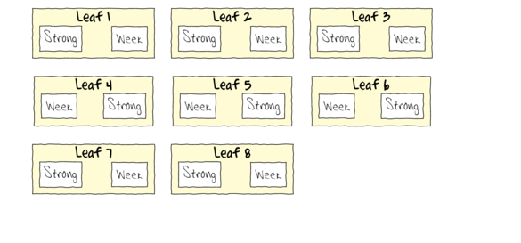
- Note that each level of the Treatment (Strong and Week) are applied to each Leaf (Block)
- Note that Treatments are randomly applied
- The Treatment effect is the mean difference between Treatment pairs per leaf
- Blocking in this way is very useful when spatial or temporal heterogeneity is likely to add noise that could make it difficualt to detect a difference between Treatments. Hence it is a way of experimentally reducing unexplained variation (compared to nesting which involves statistical reduction of unexplained variation).
Exploratory data analysis has indicated that the response variable could be normalized via a forth-root transformation.
- Fit a model for the Randomized Complete Block
- Full Effects parameterization - random intercepts model (JAGS)
number of lesionsi = βSite j(i) + εi where ε ∼ N(0,σ2)
View full effects parameterization (JAGS) codemodelString= ## write the model to a text file (I suggest you alter the path to somewhere more relevant ## to your system!) writeLines(modelString,con="../downloads/BUGSscripts/ws9.3bQ1.1a.txt") tobacco.list <- with(tobacco, list(number=NUMBER, treatment=as.numeric(TREATMENT), leaf=as.numeric(LEAF), n=nrow(tobacco), nTreat=length(levels(as.factor(TREATMENT))), nLeaf=length(levels(as.factor(LEAF))) ) ) params <- c("perc.Treat","p.decline","p.decline5","p.decline10","p.decline20","p.decline50","p.decline100","Treatment.means","beta.leaf","beta.treatment","sigma.res","sigma.leaf","sd.Resid","sd.Leaf","sd.Treatment") burnInSteps = 3000 nChains = 3 numSavedSteps = 3000 thinSteps = 100 nIter = ceiling((numSavedSteps * thinSteps)/nChains) library(R2jags) library(coda) ## tobacco.r2jags.a <- jags(data=tobacco.list, inits=NULL,#inits=list(inits,inits,inits), # since there are three chains parameters.to.save=params, model.file="../downloads/BUGSscripts/ws9.3bQ1.1a.txt", n.chains=3, n.iter=nIter, n.burnin=burnInSteps, n.thin=thinSteps )
Compiling model graph
   Resolving undeclared variables
   Allocating nodes
   Graph Size: 151

Initializing model
print(tobacco.r2jags.a)
Inference for Bugs model at "../downloads/BUGSscripts/ws9.3bQ1.1a.txt", fit using jags,
 3 chains, each with 1e+05 iterations (first 3000 discarded), n.thin = 100
 n.sims = 2910 iterations saved
                   mu.vect sd.vect    2.5%     25%     50%     75%   97.5%  Rhat n.eff
Treatment.means[1]  34.685   2.685  29.149  33.053  34.653  36.412  40.012 1.001  2900
Treatment.means[2]  26.778   2.742  21.239  25.041  26.811  28.578  32.220 1.001  2900
beta.leaf[1]        34.685   2.685  29.149  33.053  34.653  36.412  40.012 1.001  2900
beta.leaf[2]        33.656   2.814  27.994  31.863  33.737  35.492  39.055 1.001  2500
beta.leaf[3]        34.382   2.683  29.202  32.663  34.407  36.145  39.762 1.001  2900
beta.leaf[4]        32.910   2.823  27.384  31.022  32.955  34.858  38.278 1.001  2900
beta.leaf[5]        33.941   2.682  28.638  32.234  33.938  35.656  39.405 1.004   590
beta.leaf[6]        37.844   3.105  31.836  35.758  37.911  39.901  43.728 1.001  2900
beta.leaf[7]        39.568   3.597  32.746  36.978  39.646  42.186  46.379 1.001  2900
beta.leaf[8]        32.731   3.012  26.898  30.712  32.712  34.781  38.524 1.001  2600
beta.treatment[1]    0.000   0.000   0.000   0.000   0.000   0.000   0.000 1.000     1
beta.treatment[2]   -7.907   2.378 -12.693  -9.354  -7.896  -6.444  -3.224 1.001  2900
p.decline            0.999   0.037   1.000   1.000   1.000   1.000   1.000 1.029  2900
p.decline10          0.974   0.161   0.000   1.000   1.000   1.000   1.000 1.001  2900
p.decline100         0.000   0.000   0.000   0.000   0.000   0.000   0.000 1.000     1
p.decline20          0.690   0.463   0.000   0.000   1.000   1.000   1.000 1.001  2900
p.decline5           0.993   0.085   1.000   1.000   1.000   1.000   1.000 1.003  2900
p.decline50          0.000   0.019   0.000   0.000   0.000   0.000   0.000 1.291  2900
perc.Treat         -22.712   6.381 -34.921 -26.669 -22.942 -18.850  -9.835 1.001  2900
sd.Leaf              3.243   1.482   0.318   2.225   3.357   4.302   5.890 1.002  2900
sd.Resid             6.540   0.000   6.540   6.540   6.540   6.540   6.540 1.000     1
sd.Treatment         2.042   0.612   0.832   1.664   2.039   2.415   3.277 1.001  2900
sigma.leaf           3.963   2.318   0.345   2.409   3.702   5.176   9.366 1.002  2900
sigma.res            4.679   1.319   2.690   3.727   4.477   5.387   7.862 1.001  2200
deviance            92.407   6.520  80.987  87.336  92.077  97.216 105.118 1.001  2900

For each parameter, n.eff is a crude measure of effective sample size,
and Rhat is the potential scale reduction factor (at convergence, Rhat=1).

DIC info (using the rule, pD = var(deviance)/2)
pD = 21.3 and DIC = 113.7
DIC is an estimate of expected predictive error (lower deviance is better).
tobacco.mcmc.a <- tobacco.r2jags.a$BUGSoutput$sims.matrix
Note that the Leaf β are not actually the leaf means. Rather they are the intercepts for each leaf (since we have fit a random intercepts model). They represent the value of the first Treatment level (Strong) within each Leaf.
The Treatment effect thus represents the mean of the differences between the second Treatment level (Week) and these intercepts.
Indeed, the analysis assumes that there is no real interactions between the Leafs (Blocks) and the Treatment effects (within Blocks) - otherwise the mean Treatment effect would be a over simplification of the true nature of the populations. The presence of such an interaction would indicate that the Blocks (Leafs) do not all represent the same population.
View full codemodelString= ## write the model to a text file (I suggest you alter the path to somewhere more relevant ## to your system!) writeLines(modelString,con="../downloads/BUGSscripts/ws9.3bQ1.1a1.txt") tobacco.list <- with(tobacco, list(number=NUMBER, treatment=as.numeric(TREATMENT), leaf=as.numeric(LEAF), n=nrow(tobacco), nTreat=length(levels(as.factor(TREATMENT))), nLeaf=length(levels(as.factor(LEAF))) ) ) params <- c("Leaf.means","Treatment.means","beta","beta.leaf","beta.treatment","sigma.res","sd.Leaf","sd.Treatment","sd.Int","sd.Resid") adaptSteps = 1000 burnInSteps = 200 nChains = 3 numSavedSteps = 5000 thinSteps = 10 nIter = ceiling((numSavedSteps * thinSteps)/nChains) library(R2jags) ## tobacco.r2jags2 <- jags(data=tobacco.list, inits=NULL,#inits=list(inits,inits,inits), # since there are three chains parameters.to.save=params, model.file="../downloads/BUGSscripts/ws9.3bQ1.1a1.txt", n.chains=3, n.iter=nIter, n.burnin=burnInSteps, n.thin=thinSteps )
Compiling model graph
   Resolving undeclared variables
   Allocating nodes
   Graph Size: 185

Initializing model
print(tobacco.r2jags2)
Inference for Bugs model at "../downloads/BUGSscripts/ws9.3bQ1.1a1.txt", fit using jags,
 3 chains, each with 16667 iterations (first 200 discarded), n.thin = 10
 n.sims = 4941 iterations saved
                   mu.vect sd.vect     2.5%     25%     50%     75%  97.5%  Rhat n.eff
Leaf.means[1]       30.450   0.532   30.303  30.448  30.459  30.470 30.614 1.290  3600
Leaf.means[2]       28.655   1.204   28.471  28.632  28.643  28.654 28.806 1.286  4900
Leaf.means[3]       29.887   1.478   29.736  29.901  29.912  29.923 30.083 1.289  4000
Leaf.means[4]       27.075   1.181   26.895  27.070  27.082  27.092 27.231 1.286  4900
Leaf.means[5]       29.108   1.018   28.939  29.092  29.103  29.114 29.282 1.286  4900
Leaf.means[6]       36.349   0.653   36.156  36.349  36.360  36.371 36.538 1.290  3500
Leaf.means[7]       39.603   0.588   39.436  39.593  39.604  39.615 39.770 1.280  4900
Leaf.means[8]       26.843   0.776   26.659  26.830  26.841  26.852 27.026 1.284  4900
Treatment.means[1]  34.932   0.565   34.837  34.934  34.940  34.945 35.016 1.290  4000
Treatment.means[2]  27.060   0.418   26.981  27.055  27.061  27.066 27.155 1.288  4900
beta[1,1]           35.898   0.539   35.599  35.882  35.898  35.913 36.124 1.260  4900
beta[2,1]           34.126   1.993   33.856  34.101  34.117  34.133 34.333 1.286  4900
beta[3,1]           35.652   2.193   35.437  35.686  35.702  35.717 35.944 1.289  1900
beta[4,1]           26.214   1.867   25.945  26.208  26.224  26.240 26.436 1.287  4900
beta[5,1]           33.018   0.754   32.745  33.001  33.017  33.032 33.275 1.257  4900
beta[6,1]           36.723   0.714   36.450  36.712  36.728  36.743 36.974 1.285  4600
beta[7,1]           44.718   0.766   44.459  44.708  44.723  44.738 44.966 1.284  4800
beta[8,1]           33.107   0.654   32.867  33.094  33.110  33.125 33.395 1.274  4900
beta[1,2]           25.002   1.325   24.810  25.005  25.021  25.036 25.278 1.285  2900
beta[2,2]           23.184   1.023   22.912  23.152  23.168  23.184 23.419 1.282  4100
beta[3,2]           24.121   1.202   23.877  24.106  24.122  24.137 24.332 1.274  4900
beta[4,2]           27.935   0.694   27.679  27.923  27.939  27.954 28.161 1.242  4900
beta[5,2]           25.198   1.848   24.952  25.174  25.189  25.205 25.484 1.286  4900
beta[6,2]           35.975   0.974   35.719  35.978  35.993  36.008 36.267 1.279  2500
beta[7,2]           34.487   1.033   34.256  34.469  34.485  34.500 34.735 1.277  4900
beta[8,2]           20.579   1.255   20.321  20.557  20.572  20.587 20.831 1.284  4900
beta.leaf[1]         0.000   0.000    0.000   0.000   0.000   0.000  0.000 1.000     1
beta.leaf[2]        -1.795   1.636   -2.073  -1.832  -1.816  -1.801 -1.583 1.286  4300
beta.leaf[3]        -0.564   1.164   -0.821  -0.564  -0.548  -0.532 -0.299 1.282  4900
beta.leaf[4]        -3.375   1.487   -3.630  -3.393  -3.377  -3.362 -3.179 1.286  4900
beta.leaf[5]        -1.342   0.858   -1.593  -1.372  -1.356  -1.341 -1.077 1.274  3200
beta.leaf[6]         5.899   0.738    5.635   5.886   5.901   5.917  6.155 1.274  4900
beta.leaf[7]         9.153   0.843    8.915   9.129   9.145   9.160  9.406 1.280  4900
beta.leaf[8]        -3.607   1.118   -3.879  -3.634  -3.618  -3.603 -3.370 1.281  4900
beta.treatment[1]    0.000   0.000    0.000   0.000   0.000   0.000  0.000 1.000     1
beta.treatment[2]   -7.872   0.861   -7.978  -7.887  -7.879  -7.871 -7.728 1.286  4900
sd.Int               2.625   0.611    2.550   2.594   2.598   2.602  2.683 1.265   500
sd.Leaf              4.598   0.857    4.517   4.564   4.568   4.572  4.656 1.285   530
sd.Resid             6.540   0.000    6.540   6.540   6.540   6.540  6.540 1.000     1
sd.Treatment         5.578   0.488    5.466   5.566   5.571   5.577  5.641 1.254  4900
sigma.res           47.566  29.437    1.450  22.068  46.182  73.601 96.953 1.049    86
deviance           -66.217  36.598 -105.078 -91.771 -76.891 -53.566 33.084 1.048    87

For each parameter, n.eff is a crude measure of effective sample size,
and Rhat is the potential scale reduction factor (at convergence, Rhat=1).

DIC info (using the rule, pD = var(deviance)/2)
pD = 654.3 and DIC = 588.1
DIC is an estimate of expected predictive error (lower deviance is better).
View matrix parameterization (JAGS) codemodelString=" model { #Likelihood for (i in 1:n) { y[i]~dnorm(mu[i],tau.res) mu[i] <- inprod(gamma[],Z[i,]) + inprod(beta[],X[i,]) y.err[i] <- y[i] - mu[i] } #Priors and derivatives for (i in 1:nZ) { gamma[i] ~ dnorm(mu.gamma,tau.leaf) } mu.gamma ~ dnorm(0,1.0E-06) for (i in 1:nX) { beta[i] ~ dnorm(0,1.0E-6) } Treatment.means[1] <- beta[1] Treatment.means[2] <- beta[1]+beta[2] # Half-cauchy (scale=25) priors on variance tau.res <- pow(sigma.res,-2) sigma.res <-z/sqrt(chSq) z ~ dnorm(0, .0016)I(0,) chSq ~ dgamma(0.5, 0.5) tau.leaf <- pow(sigma.leaf,-2) sigma.leaf <- z.leaf/sqrt(chSq.leaf) z.leaf ~ dnorm(0, .0016)I(0,) chSq.leaf ~ dgamma(0.5, 0.5) sd.Leaf <- sd(gamma) sd.Treatment <- sd(Treatment.means) sd.Resid <- sd(y.err) } " ## write the model to a text file (I suggest you alter the path to somewhere more relevant ## to your system!) writeLines(modelString,con="../downloads/BUGSscripts/ws9.3bQ1.1b.txt") Xmat <- model.matrix(~TREATMENT, tobacco) Zmat <- model.matrix(~LEAF, tobacco) tobacco.list <- with(tobacco, list(y=NUMBER, X=Xmat, nX=ncol(Xmat), Z=Zmat, nZ=ncol(Zmat), n=nrow(tobacco) ) ) tobacco.list
$y
 [1] 35.90 25.02 34.12 23.17 35.70 24.12 26.22 27.94 33.02 25.19 35.99 36.73 34.48 44.72 20.57 33.11

$X
   (Intercept) TREATMENTWeak
1            1             0
2            1             1
3            1             0
4            1             1
5            1             0
6            1             1
7            1             0
8            1             1
9            1             0
10           1             1
11           1             1
12           1             0
13           1             1
14           1             0
15           1             1
16           1             0
attr(,"assign")
[1] 0 1
attr(,"contrasts")
attr(,"contrasts")$TREATMENT
[1] "contr.treatment"


$nX
[1] 2

$Z
   (Intercept) LEAFL2 LEAFL3 LEAFL4 LEAFL5 LEAFL6 LEAFL7 LEAFL8
1            1      0      0      0      0      0      0      0
2            1      0      0      0      0      0      0      0
3            1      1      0      0      0      0      0      0
4            1      1      0      0      0      0      0      0
5            1      0      1      0      0      0      0      0
6            1      0      1      0      0      0      0      0
7            1      0      0      1      0      0      0      0
8            1      0      0      1      0      0      0      0
9            1      0      0      0      1      0      0      0
10           1      0      0      0      1      0      0      0
11           1      0      0      0      0      1      0      0
12           1      0      0      0      0      1      0      0
13           1      0      0      0      0      0      1      0
14           1      0      0      0      0      0      1      0
15           1      0      0      0      0      0      0      1
16           1      0      0      0      0      0      0      1
attr(,"assign")
[1] 0 1 1 1 1 1 1 1
attr(,"contrasts")
attr(,"contrasts")$LEAF
[1] "contr.treatment"


$nZ
[1] 8

$n
[1] 16
params <- c("Treatment.means","gamma","beta","sigma.res","sigma.leaf","sd.Resid","sd.Leaf","sd.Treatment")
burnInSteps = 3000
nChains = 3
numSavedSteps = 3000
thinSteps = 100
nIter = ceiling((numSavedSteps * thinSteps)/nChains)

library(R2jags)
##
tobacco.r2jags.b <- jags(data=tobacco.list,
          inits=NULL,#inits=list(inits,inits,inits), # since there are three chains
          parameters.to.save=params,
          model.file="../downloads/BUGSscripts/ws9.3bQ1.1b.txt",
          n.chains=3,
          n.iter=nIter,
          n.burnin=burnInSteps,
      n.thin=thinSteps
          )
Compiling model graph
   Resolving undeclared variables
   Allocating nodes
   Graph Size: 288

Initializing model
print(tobacco.r2jags.b)
Inference for Bugs model at "../downloads/BUGSscripts/ws9.3bQ1.1b.txt", fit using jags,
 3 chains, each with 1e+05 iterations (first 3000 discarded), n.thin = 100
 n.sims = 2910 iterations saved
                   mu.vect sd.vect    2.5%    25%    50%    75%   97.5%  Rhat n.eff
Treatment.means[1]  33.486   9.390  14.235 27.827 33.589 39.395  51.137 1.001  2900
Treatment.means[2]  25.671   9.419   6.849 19.987 25.901 31.472  43.860 1.002  2900
beta[1]             33.486   9.390  14.235 27.827 33.589 39.395  51.137 1.001  2900
beta[2]             -7.815   2.377 -12.724 -9.259 -7.774 -6.342  -3.158 1.003  1200
gamma[1]             0.802   6.996 -12.693 -3.234  0.641  4.811  15.336 1.002  2900
gamma[2]            -0.723   4.474  -9.263 -3.575 -0.895  1.947   8.839 1.002  1600
gamma[3]            -0.057   4.404  -8.473 -2.878 -0.165  2.552   9.101 1.002  1200
gamma[4]            -1.703   4.521 -10.015 -4.635 -1.863  1.037   7.951 1.002  1100
gamma[5]            -0.476   4.479  -8.892 -3.343 -0.596  2.264   8.743 1.001  2400
gamma[6]             3.756   4.639  -5.926  0.900  3.928  6.736  12.630 1.002  2100
gamma[7]             5.604   4.990  -4.898  2.573  5.861  8.939  14.660 1.002  1500
gamma[8]            -1.797   4.505 -10.125 -4.771 -1.947  0.878   8.022 1.002  1700
sd.Leaf              3.798   1.820   0.412  2.604  3.849  4.884   7.482 1.002  2900
sd.Resid             4.304   0.934   2.972  3.595  4.154  4.894   6.480 1.001  2900
sd.Treatment         5.534   1.656   2.253  4.484  5.497  6.547   8.997 1.004  1000
sigma.leaf           4.599   2.747   0.444  2.812  4.221  5.832  11.175 1.001  2900
sigma.res            4.669   1.364   2.674  3.661  4.452  5.428   7.948 1.001  2900
deviance            92.603   6.931  80.944 87.315 92.201 97.366 106.748 1.001  2900

For each parameter, n.eff is a crude measure of effective sample size,
and Rhat is the potential scale reduction factor (at convergence, Rhat=1).

DIC info (using the rule, pD = var(deviance)/2)
pD = 24.0 and DIC = 116.6
DIC is an estimate of expected predictive error (lower deviance is better).
tobacco.mcmc.b <- tobacco.r2jags.b$BUGSoutput$sims.matrix
Matrix parameterization STAN coderstanString=" data{ int n; int nZ; int nX; vector [n] y; matrix [n,nX] X; matrix [n,nZ] Z; vector [nX] a0; matrix [nX,nX] A0; } parameters{ vector [nX] beta; real<lower=0> sigma; vector [nZ] gamma; real<lower=0> sigma_Z; } transformed parameters { vector [n] mu; mu <- Z*gamma + X*beta; } model{ // Priors beta ~ multi_normal(a0,A0); gamma ~ normal( 0 , sigma_Z ); sigma_Z ~ cauchy(0,25); sigma ~ cauchy(0,25); y ~ normal( mu , sigma ); } generated quantities { vector [n] y_err; real<lower=0> sd_Resid; y_err <- y - mu; sd_Resid <- sd(y_err); } " # Generate a data list Xmat <- model.matrix(~TREATMENT, data=tobacco) Zmat <- model.matrix(~-1+LEAF, data=tobacco) tobacco.list <- with(tobacco, list(y=NUMBER, Z=Zmat, X=Xmat, nX=ncol(Xmat), nZ=ncol(Zmat), n=nrow(tobacco), a0=rep(0,ncol(Xmat)), A0=diag(100000,ncol(Xmat)) ) ) # define parameters burnInSteps = 6000 nChains = 3 numSavedSteps = 3000 thinSteps = 100 nIter = burnInSteps+ceiling((numSavedSteps * thinSteps)/nChains) library(rstan) tobacco.rstan.a <- stan(data=tobacco.list, model_code=rstanString, pars=c('beta','gamma','sigma','sigma_Z', 'sd_Resid'), chains=nChains, iter=nIter, warmup=burnInSteps, thin=thinSteps, save_dso=TRUE )
TRANSLATING MODEL 'rstanString' FROM Stan CODE TO C++ CODE NOW.
COMPILING THE C++ CODE FOR MODEL 'rstanString' NOW.

SAMPLING FOR MODEL 'rstanString' NOW (CHAIN 1).

Iteration:      1 / 106000 [  0%]  (Warmup)
Iteration:   6001 / 106000 [  5%]  (Sampling)
Iteration:  16600 / 106000 [ 15%]  (Sampling)
Iteration:  27200 / 106000 [ 25%]  (Sampling)
Iteration:  37800 / 106000 [ 35%]  (Sampling)
Iteration:  48400 / 106000 [ 45%]  (Sampling)
Iteration:  59000 / 106000 [ 55%]  (Sampling)
Iteration:  69600 / 106000 [ 65%]  (Sampling)
Iteration:  80200 / 106000 [ 75%]  (Sampling)
Iteration:  90800 / 106000 [ 85%]  (Sampling)
Iteration: 101400 / 106000 [ 95%]  (Sampling)
Iteration: 106000 / 106000 [100%]  (Sampling)
#  Elapsed Time: 0.4 seconds (Warm-up)
#                30.66 seconds (Sampling)
#                31.06 seconds (Total)


SAMPLING FOR MODEL 'rstanString' NOW (CHAIN 2).

Iteration:      1 / 106000 [  0%]  (Warmup)
Iteration:   6001 / 106000 [  5%]  (Sampling)
Iteration:  16600 / 106000 [ 15%]  (Sampling)
Iteration:  27200 / 106000 [ 25%]  (Sampling)
Iteration:  37800 / 106000 [ 35%]  (Sampling)
Iteration:  48400 / 106000 [ 45%]  (Sampling)
Iteration:  59000 / 106000 [ 55%]  (Sampling)
Iteration:  69600 / 106000 [ 65%]  (Sampling)
Iteration:  80200 / 106000 [ 75%]  (Sampling)
Iteration:  90800 / 106000 [ 85%]  (Sampling)
Iteration: 101400 / 106000 [ 95%]  (Sampling)
Iteration: 106000 / 106000 [100%]  (Sampling)
#  Elapsed Time: 0.45 seconds (Warm-up)
#                10.61 seconds (Sampling)
#                11.06 seconds (Total)


SAMPLING FOR MODEL 'rstanString' NOW (CHAIN 3).

Iteration:      1 / 106000 [  0%]  (Warmup)
Iteration:   6001 / 106000 [  5%]  (Sampling)
Iteration:  16600 / 106000 [ 15%]  (Sampling)
Iteration:  27200 / 106000 [ 25%]  (Sampling)
Iteration:  37800 / 106000 [ 35%]  (Sampling)
Iteration:  48400 / 106000 [ 45%]  (Sampling)
Iteration:  59000 / 106000 [ 55%]  (Sampling)
Iteration:  69600 / 106000 [ 65%]  (Sampling)
Iteration:  80200 / 106000 [ 75%]  (Sampling)
Iteration:  90800 / 106000 [ 85%]  (Sampling)
Iteration: 101400 / 106000 [ 95%]  (Sampling)
Iteration: 106000 / 106000 [100%]  (Sampling)
#  Elapsed Time: 0.51 seconds (Warm-up)
#                9.81 seconds (Sampling)
#                10.32 seconds (Total)
print(tobacco.rstan.a)
Inference for Stan model: rstanString.
3 chains, each with iter=106000; warmup=6000; thin=100;
post-warmup draws per chain=1000, total post-warmup draws=3000.

           mean se_mean   sd   2.5%    25%    50%    75%  97.5% n_eff Rhat
beta[1]   34.92    0.04 2.36  30.28  33.54  34.93  36.37  39.72  3000    1
beta[2]   -7.89    0.04 2.40 -12.76  -9.34  -7.87  -6.45  -3.00  3000    1
gamma[1]  -0.26    0.05 2.68  -5.95  -1.79  -0.24   1.24   5.09  2656    1
gamma[2]  -1.28    0.05 2.77  -7.01  -2.95  -1.09   0.41   4.00  3000    1
gamma[3]  -0.61    0.05 2.73  -6.47  -2.16  -0.48   0.99   4.85  3000    1
gamma[4]  -2.10    0.06 2.91  -8.26  -3.95  -1.84  -0.14   3.26  2772    1
gamma[5]  -1.01    0.05 2.75  -6.80  -2.58  -0.89   0.60   4.42  3000    1
gamma[6]   2.92    0.06 3.11  -2.30   0.65   2.54   4.93   9.57  3000    1
gamma[7]   4.61    0.07 3.62  -1.08   1.77   4.40   7.03  12.33  3000    1
gamma[8]  -2.23    0.05 2.83  -8.28  -3.93  -1.92  -0.26   2.84  2938    1
sigma      4.65    0.03 1.32   2.67   3.68   4.46   5.40   7.72  2675    1
sigma_Z    4.04    0.04 2.34   0.54   2.48   3.76   5.15   9.45  3000    1
sd_Resid   4.26    0.02 0.84   2.98   3.60   4.14   4.87   5.98  2769    1
lp__     -42.06    0.08 4.10 -50.09 -44.41 -41.98 -39.80 -32.84  2574    1

Samples were drawn using NUTS(diag_e) at Fri Jan 30 11:30:36 2015.
For each parameter, n_eff is a crude measure of effective sample size,
and Rhat is the potential scale reduction factor on split chains (at
convergence, Rhat=1).
tobacco.mcmc.d <- rstan:::as.mcmc.list.stanfit(tobacco.rstan.a) tobacco.mcmc.df.d <- as.data.frame(extract(tobacco.rstan.a))
library(plyr)
#Finite-population standard deviations
## Leaf
library(coda)

sd.leaf <- tobacco.mcmc.df.d[,3:10]
SD.leaf <- apply(sd.leaf,1,sd)
data.frame(mean=mean(SD.leaf), median=median(SD.leaf), HPDinterval(as.mcmc(SD.leaf)), HPDinterval(as.mcmc(SD.leaf),p=0.68))
      mean median lower upper lower.1 upper.1
var1 3.288  3.385 0.364 5.676   1.891   4.835
#Treatment
treatments <- NULL
treatments <- cbind(tobacco.mcmc.df.d[,'beta.1'],
                 tobacco.mcmc.df.d[,'beta.1']+tobacco.mcmc.df.d[,'beta.2'])
sd.treatment <- apply(treatments,1,sd)
data.frame(mean=mean(sd.treatment), median=median(sd.treatment), HPDinterval(as.mcmc(sd.treatment)), HPDinterval(as.mcmc(sd.treatment),p=0.68))
      mean median lower upper lower.1 upper.1
var1 5.587  5.565 2.288 9.159   3.965    7.02
- Full Effects parameterization - random intercepts model (JAGS)
- Before fully exploring the parameters, it is prudent to examine the convergence and mixing diagnostics.
Chose either any of the parameterizations (they should yield much the same) - although it is sometimes useful to explore the
different performances of effects vs matrix and JAGS vs STAN.
Full effects parameterization JAGS code
library(coda)
plot(as.mcmc(tobacco.r2jags.a))
Error: invalid 'length' argument
preds <- c("beta.leaf[1]","beta.treatment[2]", "sigma.res", "sigma.leaf")

autocorr.diag(as.mcmc(tobacco.r2jags.a)[, preds])
Error: incorrect number of dimensions
raftery.diag(as.mcmc(tobacco.r2jags.a))
Quantile (q) = 0.025
Accuracy (r) = +/- 0.005
Probability (s) = 0.95

You need a sample size of at least 3746 with these values of q, r and s
Matrix parameterization JAGS codelibrary(coda) plot(as.mcmc(tobacco.r2jags.b))
Error: invalid 'length' argument
preds <- c("beta[1]","beta[2]", "sigma.res", "sigma.leaf")

autocorr.diag(as.mcmc(tobacco.r2jags.b)[, preds])
Error: incorrect number of dimensions
raftery.diag(as.mcmc(tobacco.r2jags.b))
Quantile (q) = 0.025
Accuracy (r) = +/- 0.005
Probability (s) = 0.95

You need a sample size of at least 3746 with these values of q, r and s
Matrix parameterization STAN codelibrary(coda) preds <- c("beta[1]", "beta[2]", "sigma", "sigma_Z") plot(tobacco.mcmc.d)


autocorr.diag(tobacco.mcmc.d[, preds])
           beta[1]   beta[2]    sigma   sigma_Z
Lag 0     1.000000  1.000000  1.00000  1.000000
Lag 100  -0.018868 -0.006011  0.03265 -0.002893
Lag 500  -0.005449  0.005173 -0.02275 -0.018524
Lag 1000 -0.007707  0.017508 -0.04330  0.022630
Lag 5000 -0.011061  0.019536  0.00145  0.007100
raftery.diag(tobacco.mcmc.d)
[[1]]

Quantile (q) = 0.025
Accuracy (r) = +/- 0.005
Probability (s) = 0.95

You need a sample size of at least 3746 with these values of q, r and s

[[2]]

Quantile (q) = 0.025
Accuracy (r) = +/- 0.005
Probability (s) = 0.95

You need a sample size of at least 3746 with these values of q, r and s

[[3]]

Quantile (q) = 0.025
Accuracy (r) = +/- 0.005
Probability (s) = 0.95

You need a sample size of at least 3746 with these values of q, r and s
- Summary figure time
Matrix parameterization JAGS code
preds <- c('beta[1]','beta[2]')
coefs <- tobacco.r2jags.b$BUGSoutput$sims.matrix[,preds]

newdata <- data.frame(TREAT=levels(tobacco$TREAT))
Xmat <- model.matrix(~TREAT, newdata)
pred <- coefs %*% t(Xmat)
library(plyr)
newdata <- cbind(newdata, adply(pred, 2, function(x) {
   data.frame(Median=median(x), HPDinterval(as.mcmc(x)), HPDinterval(as.mcmc(x), p=0.68))
}))
newdata
   TREAT X1 Median  lower upper lower.1 upper.1
1 Strong  1  33.59 14.040 50.36   25.63   42.90
2   Weak  2  25.90  5.961 42.52   17.06   34.29
library(ggplot2)
p1 <- ggplot(newdata, aes(y=Median, x=TREAT)) +
   geom_linerange(aes(ymin=lower, ymax=upper), show_guide=FALSE)+
   geom_linerange(aes(ymin=lower.1, ymax=upper.1), size=2,show_guide=FALSE)+
   geom_point(size=4, shape=21, fill="white")+
   scale_y_continuous('Number of lessions')+
   theme_classic()+
   theme(axis.title.y=element_text(vjust=2,size=rel(1.2)),
         axis.title.x=element_text(vjust=-2,size=rel(1.2)),
                 plot.margin=unit(c(0.5,0.5,2,2), 'lines'))

preds <- c('sd.Resid','sd.Treatment','sd.Leaf')
tobacco.sd <- adply(tobacco.mcmc.b[,preds],2,function(x) {
   data.frame(mean=mean(x), median=median(x), HPDinterval(as.mcmc(x)), HPDinterval(as.mcmc(x),p=0.68))
})
head(tobacco.sd)
            X1  mean median    lower upper lower.1 upper.1
1     sd.Resid 4.304  4.154 2.785436 6.061   3.105   4.837
2 sd.Treatment 5.534  5.497 2.149849 8.824   4.020   7.137
3      sd.Leaf 3.798  3.849 0.005277 6.582   2.198   5.537
rownames(tobacco.sd) <- c("Residuals", "Treatment", "Leaf")
tobacco.sd$name <- factor(c("Residuals", "Treatment", "Leaf"), levels=c("Residuals", "Treatment", "Leaf"))
tobacco.sd$Perc <- tobacco.sd$median/sum(tobacco.sd$median)

p2<-ggplot(tobacco.sd,aes(y=name, x=median))+
  geom_vline(xintercept=0,linetype="dashed")+
  geom_hline(xintercept=0)+
  scale_x_continuous("Finite population \nvariance components (sd)")+
  geom_errorbarh(aes(xmin=lower.1, xmax=upper.1), height=0, size=1)+
  geom_errorbarh(aes(xmin=lower, xmax=upper), height=0, size=1.5)+
  geom_point(size=3, shape=21, fill='white')+
  geom_text(aes(label=sprintf("(%4.1f%%)",Perc),vjust=-1))+
  theme_classic()+
  theme(axis.title.y=element_blank(),
        axis.text.y=element_text(size=rel(1.2),hjust=1))

library(gridExtra)
grid.arrange(p1,p2,ncol=2)
