Workshop 9.4b - Mixed effects (Multilevel models): Split-plot and complex repeated measures designs (Bayesian)
31 Jan 2015
Split-plot ANOVA (Mixed effects) references
- McCarthy (2007) - Chpt ?
- Kery (2010) - Chpt ?
- Gelman & Hill (2007) - Chpt ?
- Logan (2010) - Chpt 13
- Quinn & Keough (2002) - Chpt 10
Split-plot
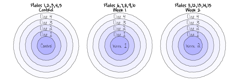
Split-plotIn an attempt to understand the effects on marine animals of short-term exposure to toxic substances, such as might occur following a spill, or a major increase in storm water flows, a it was decided to examine the toxicant in question, Copper, as part of a field experiment in Honk Kong. The experiment consisted of small sources of Cu (small, hemispherical plaster blocks, impregnated with copper), which released the metal into sea water over 4 or 5 days. The organism whose response to Cu was being measured was a small, polychaete worm, Hydroides, that attaches to hard surfaces in the sea, and is one of the first species to colonize any surface that is submerged. The biological questions focused on whether the timing of exposure to Cu affects the overall abundance of these worms. The time period of interest was the first or second week after a surface being available.
The experimental setup consisted of sheets of black perspex (settlement plates), which provided good surfaces for these worms. Each plate had a plaster block bolted to its centre, and the dissolving block would create a gradient of [Cu] across the plate. Over the two weeks of the experiment, a given plate would have pl ain plaster blocks (Control) or a block containing copper in the first week, followed by a plain block, or a plain block in the first week, followed by a dose of copper in the second week. After two weeks in the water, plates were removed and counted back in the laboratory. Without a clear idea of how sensitive these worms are to copper, an effect of the treatments might show up as an overall difference in the density of worms across a plate, or it could show up as a gradient in abundance across the plate, with a different gradient in different treatments. Therefore, on each plate, the density of worms (#/cm2) was recorded at each of four distances from the center of the plate.
Download Copper data set| Format of copper.csv data file | |||||||||||||||||
|---|---|---|---|---|---|---|---|---|---|---|---|---|---|---|---|---|---|
|
 |
copper <- read.table('../downloads/data/copper.csv', header=T, sep=',', strip.white=T)
head(copper)
   COPPER PLATE DIST WORMS
1 control   200    4 11.50
2 control   200    3 13.00
3 control   200    2 13.50
4 control   200    1 12.00
5 control    39    4 17.75
6 control    39    3 13.75
library(R2jags)
library(rstan)
library(coda)
The Plates are the "random" groups. Within each Plate, all levels of the Distance factor occur (this is a within group factor). Each Plate can only be of one of the three levels of the Copper treatment. This is therefore a within group (nested) factor. Traditionally, this mixture of nested and randomized block design would be called a partly nested or split-plot design.
In Bayesian (multilevel modeling) terms, this is a multi-level model with one hierarchical level the Plates means and another representing the Copper treatment means (based on the Plate means).
Exploratory data analysis has indicated that the response variable could be normalized via a forth-root transformation.
- Fit a model for Randomized Complete Block
- Effects parameterization - random intercepts model (JAGS)
number of lesionsi = βSite j(i) + εi where ε ∼ N(0,σ2)treating Distance as a factor
View full codemodelString= ## write the model to a text file (I suggest you alter the path to somewhere more relevant ## to your system!) writeLines(modelString,con="../downloads/BUGSscripts/ws9.9bQ2.1a.txt")
#sort the data set so that the copper treatments are in a more logical order
copper.sort <- copper[order(copper$COPPER),]
copper.sort$COPPER <- factor(copper.sort$COPPER, levels = c("control", "Week 1", "Week 2"))
copper.sort$PLATE <- factor(copper.sort$PLATE, levels=unique(copper.sort$PLATE))
cu <- with(copper.sort,COPPER[match(unique(PLATE),PLATE)])
cu <- factor(cu, levels=c("control", "Week 1", "Week 2"))
copper.list <- with(copper.sort,
                         list(worms=WORMS,
                           dist=as.numeric(DIST),
               plate=as.numeric(PLATE),
                           copper=factor(as.numeric(cu)),
               cu=as.numeric(COPPER),
                           nDist=length(levels(as.factor(DIST))),
                           nPlate=length(levels(as.factor(PLATE))),
                           nCopper=length(levels(cu)),
                           n=nrow(copper.sort)
                           )
                           )
params <- c("g0","gamma.copper",
                  "beta.plate",
          "beta.dist",
                  "beta.CopperDist",
                  "Copper.means","Dist.means","CopperDist.means",
                  "sd.Dist","sd.Copper","sd.Plate","sd.Resid","sd.CopperDist",
                  "sigma.res","sigma.plate","sigma.copper","sigma.dist","sigma.copperdist"
                  )
adaptSteps = 1000
burnInSteps = 2000
nChains = 3
numSavedSteps = 5000
thinSteps = 10
nIter = ceiling((numSavedSteps * thinSteps)/nChains)

library(R2jags)
##
copper.r2jags.a <- jags(data=copper.list,
                                 inits=NULL, # since there are three chains
          parameters.to.save=params,
          model.file="../downloads/BUGSscripts/ws9.9bQ2.1a.txt",
          n.chains=3,
          n.iter=nIter,
          n.burnin=burnInSteps,
      n.thin=thinSteps
          )
Compiling model graph
   Resolving undeclared variables
   Allocating nodes
   Graph Size: 458

Initializing model
print(copper.r2jags.a)
Inference for Bugs model at "../downloads/BUGSscripts/ws9.9bQ2.1a.txt", fit using jags, 3 chains, each with 16667 iterations (first 2000 discarded), n.thin = 10 n.sims = 4401 iterations saved mu.vect sd.vect 2.5% 25% 50% 75% 97.5% Rhat n.eff Copper.means[1] 10.853 0.720 9.410 10.381 10.859 11.321 12.235 1.001 3700 Copper.means[2] 6.966 0.684 5.671 6.517 6.967 7.412 8.318 1.001 3800 Copper.means[3] 0.493 0.690 -0.874 0.037 0.499 0.947 1.839 1.002 1500 CopperDist.means[1,1] 10.853 0.720 9.410 10.381 10.859 11.321 12.235 1.001 3700 CopperDist.means[2,1] 6.966 0.684 5.671 6.517 6.967 7.412 8.318 1.001 3800 CopperDist.means[3,1] 0.493 0.690 -0.874 0.037 0.499 0.947 1.839 1.002 1500 CopperDist.means[1,2] 12.008 0.676 10.668 11.563 12.018 12.459 13.309 1.001 3500 CopperDist.means[2,2] 8.405 0.674 7.055 7.963 8.406 8.854 9.687 1.001 4400 CopperDist.means[3,2] 1.579 0.679 0.255 1.121 1.584 2.026 2.908 1.001 4400 CopperDist.means[1,3] 12.428 0.642 11.152 12.018 12.414 12.838 13.708 1.001 2700 CopperDist.means[2,3] 8.591 0.683 7.245 8.135 8.586 9.052 9.951 1.001 4400 CopperDist.means[3,3] 3.932 0.681 2.586 3.485 3.920 4.380 5.298 1.001 4400 CopperDist.means[1,4] 13.523 0.708 12.190 13.032 13.531 13.989 14.896 1.001 2500 CopperDist.means[2,4] 10.088 0.676 8.750 9.641 10.078 10.546 11.434 1.001 4400 CopperDist.means[3,4] 7.543 0.720 6.117 7.056 7.557 8.034 8.912 1.001 4400 Dist.means[1] 6.107 0.366 5.367 5.869 6.115 6.340 6.827 1.002 4400 Dist.means[2] 7.262 0.798 5.725 6.724 7.267 7.800 8.811 1.001 4400 Dist.means[3] 7.682 0.779 6.113 7.172 7.691 8.187 9.228 1.001 4400 Dist.means[4] 8.777 0.826 7.159 8.223 8.754 9.324 10.417 1.001 3500 beta.CopperDist[1,1] 0.000 0.000 0.000 0.000 0.000 0.000 0.000 1.000 1 beta.CopperDist[2,1] 0.000 0.000 0.000 0.000 0.000 0.000 0.000 1.000 1 beta.CopperDist[3,1] 0.000 0.000 0.000 0.000 0.000 0.000 0.000 1.000 1 beta.CopperDist[1,2] 0.000 0.000 0.000 0.000 0.000 0.000 0.000 1.000 1 beta.CopperDist[2,2] 0.284 1.240 -2.158 -0.561 0.274 1.106 2.751 1.001 4400 beta.CopperDist[3,2] -0.068 1.207 -2.480 -0.874 -0.078 0.760 2.271 1.001 3700 beta.CopperDist[1,3] 0.000 0.000 0.000 0.000 0.000 0.000 0.000 1.000 1 beta.CopperDist[2,3] 0.050 1.214 -2.305 -0.756 0.051 0.841 2.413 1.001 3900 beta.CopperDist[3,3] 1.865 1.198 -0.556 1.074 1.873 2.670 4.279 1.001 3300 beta.CopperDist[1,4] 0.000 0.000 0.000 0.000 0.000 0.000 0.000 1.000 1 beta.CopperDist[2,4] 0.452 1.206 -1.862 -0.367 0.463 1.272 2.824 1.001 4100 beta.CopperDist[3,4] 4.381 1.332 1.695 3.507 4.404 5.274 6.975 1.002 1700 beta.dist[1] 0.000 0.000 0.000 0.000 0.000 0.000 0.000 1.000 1 beta.dist[2] 1.155 0.875 -0.570 0.573 1.158 1.737 2.857 1.001 4400 beta.dist[3] 1.575 0.874 -0.170 1.001 1.585 2.135 3.320 1.001 4400 beta.dist[4] 2.670 0.911 0.926 2.069 2.660 3.274 4.489 1.001 4400 beta.plate[1] 10.968 0.761 9.466 10.450 10.967 11.482 12.429 1.001 4400 beta.plate[2] 11.627 0.875 9.934 11.039 11.618 12.213 13.359 1.001 3400 beta.plate[3] 10.449 0.786 8.825 9.918 10.476 10.998 11.951 1.001 4400 beta.plate[4] 10.505 0.784 8.885 10.000 10.528 11.031 12.011 1.001 4400 beta.plate[5] 10.728 0.759 9.153 10.242 10.743 11.233 12.223 1.002 4400 beta.plate[6] 6.861 0.720 5.438 6.385 6.857 7.329 8.312 1.001 4400 beta.plate[7] 6.505 0.763 4.948 6.012 6.509 7.014 7.976 1.001 4400 beta.plate[8] 7.245 0.741 5.845 6.743 7.233 7.753 8.734 1.001 2900 beta.plate[9] 7.107 0.724 5.709 6.613 7.100 7.582 8.560 1.001 4400 beta.plate[10] 7.129 0.736 5.700 6.640 7.123 7.618 8.582 1.001 4400 beta.plate[11] 0.420 0.736 -1.026 -0.071 0.421 0.910 1.876 1.001 2500 beta.plate[12] 0.343 0.737 -1.091 -0.146 0.340 0.848 1.790 1.003 980 beta.plate[13] 0.387 0.737 -1.022 -0.108 0.393 0.879 1.808 1.002 1300 beta.plate[14] 0.707 0.738 -0.735 0.215 0.709 1.188 2.144 1.001 3500 beta.plate[15] 0.621 0.736 -0.835 0.135 0.623 1.109 2.066 1.002 1700 g0 10.853 0.720 9.410 10.381 10.859 11.321 12.235 1.001 3700 gamma.copper[1] 0.000 0.000 0.000 0.000 0.000 0.000 0.000 1.000 1 gamma.copper[2] -3.886 0.986 -5.802 -4.551 -3.875 -3.221 -1.907 1.002 1800 gamma.copper[3] -10.360 0.995 -12.307 -11.007 -10.357 -9.709 -8.362 1.001 3900 sd.Copper 5.256 0.495 4.244 4.936 5.251 5.578 6.246 1.001 2800 sd.CopperDist 1.484 0.351 0.817 1.248 1.477 1.714 2.202 1.001 3500 sd.Dist 1.208 0.360 0.511 0.962 1.205 1.448 1.937 1.001 4400 sd.Plate 0.528 0.271 0.045 0.326 0.528 0.724 1.048 1.004 1400 sd.Resid 4.304 0.000 4.304 4.304 4.304 4.304 4.304 1.000 1 sigma.copper 29.628 25.472 2.924 8.959 20.406 44.181 91.539 1.001 2800 sigma.copperdist 2.660 1.611 0.912 1.690 2.263 3.160 6.733 1.001 3200 sigma.dist 5.912 12.445 0.133 0.880 1.769 4.373 47.253 1.015 300 sigma.plate 0.587 0.334 0.050 0.343 0.560 0.795 1.318 1.003 1700 sigma.res 1.408 0.166 1.121 1.289 1.398 1.511 1.761 1.002 2300 deviance 209.192 8.606 193.679 203.023 208.938 214.934 226.967 1.002 1400 For each parameter, n.eff is a crude measure of effective sample size, and Rhat is the potential scale reduction factor (at convergence, Rhat=1). DIC info (using the rule, pD = var(deviance)/2) pD = 37.0 and DIC = 246.2 DIC is an estimate of expected predictive error (lower deviance is better). - Matrix parameterization - random intercepts model (JAGS)
number of lesionsi = βSite j(i) + εi where ε ∼ N(0,σ2)treating Distance as a factor
View full codeWe can perform generate the finite-population standard deviation posteriors within RmodelString=" model { #Likelihood for (i in 1:n) { y[i]~dnorm(mu[i],tau.res) mu[i] <- inprod(beta[],X[i,]) + inprod(gamma[],Z[i,]) y.err[i] <- y[i] - mu[1] } #Priors and derivatives for (i in 1:nZ) { gamma[i] ~ dnorm(0,tau.plate) } for (i in 1:nX) { beta[i] ~ dnorm(0,1.0E-06) } tau.res <- pow(sigma.res,-2) sigma.res <- z/sqrt(chSq) z ~ dnorm(0, .0016)I(0,) chSq ~ dgamma(0.5, 0.5) tau.plate <- pow(sigma.plate,-2) sigma.plate <- z.plate/sqrt(chSq.plate) z.plate ~ dnorm(0, .0016)I(0,) chSq.plate ~ dgamma(0.5, 0.5) } " ## write the model to a text file (I suggest you alter the path to somewhere more relevant ## to your system!) writeLines(modelString,con="../downloads/BUGSscripts/ws9.4bQ2.1b.txt") #sort the data set so that the copper treatments are in a more logical order library(dplyr) copper$DIST <- factor(copper$DIST) copper$PLATE <- factor(copper$PLATE) copper.sort <- arrange(copper,COPPER,PLATE,DIST) Xmat <- model.matrix(~COPPER*DIST, data=copper.sort) Zmat <- model.matrix(~-1+PLATE, data=copper.sort) copper.list <- list(y=copper.sort$WORMS, X=Xmat, nX=ncol(Xmat), Z=Zmat, nZ=ncol(Zmat), n=nrow(copper.sort) ) params <- c("beta","gamma", "sigma.res","sigma.plate") burnInSteps = 3000 nChains = 3 numSavedSteps = 3000 thinSteps = 100 nIter = ceiling((numSavedSteps * thinSteps)/nChains) library(R2jags) library(coda) ## copper.r2jags.b <- jags(data=copper.list, inits=NULL, # since there are three chains parameters.to.save=params, model.file="../downloads/BUGSscripts/ws9.4bQ2.1b.txt", n.chains=3, n.iter=nIter, n.burnin=burnInSteps, n.thin=thinSteps )
Compiling model graph
   Resolving undeclared variables
   Allocating nodes
   Graph Size: 1971

Initializing model
print(copper.r2jags.b)
Inference for Bugs model at "../downloads/BUGSscripts/ws9.4bQ2.1b.txt", fit using jags,
 3 chains, each with 1e+05 iterations (first 3000 discarded), n.thin = 100
 n.sims = 2910 iterations saved
            mu.vect sd.vect    2.5%     25%     50%     75%   97.5%  Rhat n.eff
beta[1]      10.849   0.684   9.531  10.377  10.857  11.304  12.152 1.002  1200
beta[2]      -3.617   0.977  -5.522  -4.272  -3.608  -2.979  -1.701 1.003   740
beta[3]     -10.573   0.976 -12.521 -11.215 -10.588  -9.909  -8.713 1.002  1900
beta[4]       1.161   0.877  -0.575   0.588   1.157   1.759   2.852 1.001  2900
beta[5]       1.552   0.885  -0.147   0.950   1.550   2.160   3.270 1.003   690
beta[6]       2.712   0.894   0.923   2.118   2.715   3.286   4.471 1.001  2900
beta[7]      -0.041   1.274  -2.579  -0.876  -0.004   0.828   2.370 1.001  2900
beta[8]       0.007   1.241  -2.452  -0.810  -0.007   0.831   2.453 1.001  2900
beta[9]      -0.264   1.237  -2.641  -1.084  -0.241   0.529   2.223 1.002  1300
beta[10]      2.175   1.244  -0.309   1.332   2.181   2.953   4.666 1.001  2900
beta[11]      0.066   1.279  -2.410  -0.760   0.080   0.889   2.605 1.001  2900
beta[12]      4.870   1.260   2.376   4.055   4.890   5.696   7.346 1.011  2900
gamma[1]      0.156   0.490  -0.774  -0.122   0.095   0.419   1.276 1.001  2900
gamma[2]     -0.140   0.492  -1.214  -0.407  -0.088   0.141   0.805 1.001  2900
gamma[3]      0.285   0.511  -0.606  -0.029   0.201   0.581   1.435 1.001  2900
gamma[4]     -0.423   0.547  -1.665  -0.732  -0.335  -0.030   0.469 1.001  2900
gamma[5]     -0.360   0.531  -1.518  -0.655  -0.275  -0.006   0.525 1.002  1300
gamma[6]      0.765   0.664  -0.170   0.217   0.677   1.193   2.238 1.001  2900
gamma[7]     -0.153   0.493  -1.219  -0.430  -0.091   0.117   0.781 1.003   850
gamma[8]     -0.491   0.558  -1.786  -0.829  -0.397  -0.067   0.370 1.001  2900
gamma[9]      0.138   0.497  -0.810  -0.145   0.082   0.412   1.255 1.001  2900
gamma[10]    -0.106   0.486  -1.120  -0.386  -0.061   0.160   0.877 1.002  1500
gamma[11]    -0.148   0.495  -1.204  -0.415  -0.096   0.128   0.816 1.002  1100
gamma[12]     0.213   0.503  -0.710  -0.076   0.152   0.488   1.308 1.003   760
gamma[13]     0.118   0.488  -0.886  -0.145   0.079   0.388   1.178 1.002  2200
gamma[14]     0.121   0.492  -0.871  -0.145   0.081   0.385   1.185 1.001  2900
gamma[15]    -0.092   0.502  -1.197  -0.359  -0.055   0.183   0.902 1.002  1800
sigma.plate   0.588   0.328   0.044   0.352   0.572   0.788   1.287 1.003  1600
sigma.res     1.397   0.164   1.102   1.284   1.386   1.502   1.745 1.001  2900
deviance    208.815   8.504 193.162 202.760 208.517 214.590 226.162 1.001  2300

For each parameter, n.eff is a crude measure of effective sample size,
and Rhat is the potential scale reduction factor (at convergence, Rhat=1).

DIC info (using the rule, pD = var(deviance)/2)
pD = 36.2 and DIC = 245.0
DIC is an estimate of expected predictive error (lower deviance is better).
copper.mcmc.b <- as.mcmc(copper.r2jags.b$BUGSoutput$sims.matrix)
View full codecopper.sort <- arrange(copper,COPPER,PLATE,DIST) nms <- colnames(copper.mcmc.b) pred <- grep('beta|gamma',nms) coefs <- copper.mcmc.b[,pred] newdata <- copper.sort #unique(subset(copper, select=c('COPPER','DIST','PLATE'))) Amat <- cbind(model.matrix(~COPPER*DIST, newdata),model.matrix(~-1+PLATE, newdata)) pred <- coefs %*% t(Amat) y.err <- t(copper.sort$WORMS - t(pred)) a<-apply(y.err, 1,sd) resid.sd <- data.frame(Source='Resid',Median=median(a), HPDinterval(as.mcmc(a)), HPDinterval(as.mcmc(a), p=0.68)) ## Fixed effects nms <- colnames(copper.mcmc.b) copper.mcmc.b.beta <- copper.mcmc.b[,grep('beta',nms)] assign <- attr(Xmat, 'assign') nms <- attr(terms(model.frame(~COPPER*DIST, copper.sort)),'term.labels') fixed.sd <- NULL for (i in 1:max(assign)) { w <- which(i==assign) fixed.sd<-cbind(fixed.sd, apply(copper.mcmc.b.beta[,w],1,sd)) } library(plyr) fixed.sd <-adply(fixed.sd,2,function(x) { data.frame(Median=median(x), HPDinterval(as.mcmc(x)), HPDinterval(as.mcmc(x), p=0.68)) }) fixed.sd<- cbind(Source=nms, fixed.sd) # Variances nms <- colnames(copper.mcmc.b) copper.mcmc.b.gamma <- copper.mcmc.b[,grep('gamma',nms)] assign <- attr(Zmat, 'assign') nms <- attr(terms(model.frame(~-1+PLATE, copper.sort)),'term.labels') random.sd <- NULL for (i in 1:max(assign)) { w <- which(i==assign) random.sd<-cbind(random.sd, apply(copper.mcmc.b.gamma[,w],1,sd)) } library(plyr) random.sd <-adply(random.sd,2,function(x) { data.frame(Median=median(x), HPDinterval(as.mcmc(x)), HPDinterval(as.mcmc(x), p=0.68)) }) random.sd<- cbind(Source=nms, random.sd) (copper.sd <- rbind(subset(fixed.sd, select=-X1), subset(random.sd, select=-X1), resid.sd))
          Source Median     lower  upper lower.1 upper.1
1         COPPER 4.9703 3.6177274 6.4345  4.2476  5.6256
2           DIST 0.9303 0.1402592 1.6415  0.5160  1.3082
3    COPPER:DIST 2.2198 1.3338084 3.1178  1.7949  2.6786
4          PLATE 0.5333 0.0002546 0.9595  0.2442  0.7985
var1       Resid 1.3648 1.1950027 1.5576  1.2624  1.4503
- Matrix parameterization - random intercepts model (STAN)
View full coderstanString=" data{ int n; int nZ; int nX; vector [n] y; matrix [n,nX] X; matrix [n,nZ] Z; vector [nX] a0; matrix [nX,nX] A0; } parameters{ vector [nX] beta; real<lower=0> sigma; vector [nZ] gamma; real<lower=0> sigma_Z; } transformed parameters { vector [n] mu; mu <- X*beta + Z*gamma; } model{ // Priors beta ~ multi_normal(a0,A0); gamma ~ normal( 0 , sigma_Z ); sigma_Z ~ cauchy(0,25); sigma ~ cauchy(0,25); y ~ normal( mu , sigma ); } generated quantities { vector [n] y_err; real<lower=0> sd_Resid; y_err <- y - mu; sd_Resid <- sd(y_err); } " #sort the data set so that the copper treatments are in a more logical order library(dplyr) copper$DIST <- factor(copper$DIST) copper$PLATE <- factor(copper$PLATE) copper.sort <- arrange(copper,COPPER,PLATE,DIST) Xmat <- model.matrix(~COPPER*DIST, data=copper.sort) Zmat <- model.matrix(~-1+PLATE, data=copper.sort) copper.list <- list(y=copper.sort$WORMS, X=Xmat, nX=ncol(Xmat), Z=Zmat, nZ=ncol(Zmat), n=nrow(copper.sort), a0=rep(0,ncol(Xmat)), A0=diag(100000,ncol(Xmat)) ) params <- c("beta","gamma", "sigma","sigma_Z") burnInSteps = 3000 nChains = 3 numSavedSteps = 3000 thinSteps = 100 nIter = ceiling((numSavedSteps * thinSteps)/nChains) library(rstan) library(coda) ## copper.rstan.a <- stan(data=copper.list, model_code=rstanString, pars=c("beta","gamma","sigma","sigma_Z"), chains=nChains, iter=nIter, warmup=burnInSteps, thin=thinSteps, save_dso=TRUE )
TRANSLATING MODEL 'rstanString' FROM Stan CODE TO C++ CODE NOW.
COMPILING THE C++ CODE FOR MODEL 'rstanString' NOW.

SAMPLING FOR MODEL 'rstanString' NOW (CHAIN 1).

Iteration:     1 / 100000 [  0%]  (Warmup)
Iteration:  3001 / 100000 [  3%]  (Sampling)
Iteration: 13000 / 100000 [ 13%]  (Sampling)
Iteration: 23000 / 100000 [ 23%]  (Sampling)
Iteration: 33000 / 100000 [ 33%]  (Sampling)
Iteration: 43000 / 100000 [ 43%]  (Sampling)
Iteration: 53000 / 100000 [ 53%]  (Sampling)
Iteration: 63000 / 100000 [ 63%]  (Sampling)
Iteration: 73000 / 100000 [ 73%]  (Sampling)
Iteration: 83000 / 100000 [ 83%]  (Sampling)
Iteration: 93000 / 100000 [ 93%]  (Sampling)
Iteration: 100000 / 100000 [100%]  (Sampling)
#  Elapsed Time: 1.58 seconds (Warm-up)
#                64.79 seconds (Sampling)
#                66.37 seconds (Total)


SAMPLING FOR MODEL 'rstanString' NOW (CHAIN 2).

Iteration:     1 / 100000 [  0%]  (Warmup)
Iteration:  3001 / 100000 [  3%]  (Sampling)
Iteration: 13000 / 100000 [ 13%]  (Sampling)
Iteration: 23000 / 100000 [ 23%]  (Sampling)
Iteration: 33000 / 100000 [ 33%]  (Sampling)
Iteration: 43000 / 100000 [ 43%]  (Sampling)
Iteration: 53000 / 100000 [ 53%]  (Sampling)
Iteration: 63000 / 100000 [ 63%]  (Sampling)
Iteration: 73000 / 100000 [ 73%]  (Sampling)
Iteration: 83000 / 100000 [ 83%]  (Sampling)
Iteration: 93000 / 100000 [ 93%]  (Sampling)
Iteration: 100000 / 100000 [100%]  (Sampling)
#  Elapsed Time: 1.52 seconds (Warm-up)
#                73.33 seconds (Sampling)
#                74.85 seconds (Total)


SAMPLING FOR MODEL 'rstanString' NOW (CHAIN 3).

Iteration:     1 / 100000 [  0%]  (Warmup)
Iteration:  3001 / 100000 [  3%]  (Sampling)
Iteration: 13000 / 100000 [ 13%]  (Sampling)
Iteration: 23000 / 100000 [ 23%]  (Sampling)
Iteration: 33000 / 100000 [ 33%]  (Sampling)
Iteration: 43000 / 100000 [ 43%]  (Sampling)
Iteration: 53000 / 100000 [ 53%]  (Sampling)
Iteration: 63000 / 100000 [ 63%]  (Sampling)
Iteration: 73000 / 100000 [ 73%]  (Sampling)
Iteration: 83000 / 100000 [ 83%]  (Sampling)
Iteration: 93000 / 100000 [ 93%]  (Sampling)
Iteration: 100000 / 100000 [100%]  (Sampling)
#  Elapsed Time: 2.35 seconds (Warm-up)
#                69.92 seconds (Sampling)
#                72.27 seconds (Total)
print(copper.rstan.a)
Inference for Stan model: rstanString.
3 chains, each with iter=1e+05; warmup=3000; thin=100;
post-warmup draws per chain=970, total post-warmup draws=2910.

            mean se_mean   sd   2.5%    25%    50%    75%  97.5% n_eff Rhat
beta[1]    10.86    0.01 0.69   9.49  10.40  10.86  11.34  12.21  2910    1
beta[2]    -3.59    0.02 0.98  -5.49  -4.28  -3.59  -2.93  -1.70  2670    1
beta[3]   -10.58    0.02 0.98 -12.51 -11.23 -10.58  -9.93  -8.63  2910    1
beta[4]     1.15    0.02 0.91  -0.66   0.54   1.16   1.75   2.95  2672    1
beta[5]     1.56    0.02 0.89  -0.22   0.96   1.56   2.12   3.35  2909    1
beta[6]     2.69    0.02 0.90   0.94   2.10   2.69   3.28   4.50  2807    1
beta[7]    -0.06    0.02 1.29  -2.58  -0.92  -0.08   0.80   2.47  2670    1
beta[8]     0.03    0.02 1.27  -2.52  -0.80   0.02   0.86   2.50  2910    1
beta[9]    -0.30    0.02 1.27  -2.74  -1.16  -0.31   0.54   2.24  2910    1
beta[10]    2.19    0.02 1.25  -0.26   1.37   2.20   3.03   4.60  2910    1
beta[11]    0.06    0.02 1.27  -2.49  -0.78   0.06   0.91   2.51  2892    1
beta[12]    4.88    0.02 1.25   2.32   4.06   4.92   5.70   7.26  2910    1
gamma[1]    0.15    0.01 0.49  -0.80  -0.12   0.11   0.39   1.21  2910    1
gamma[2]   -0.13    0.01 0.50  -1.23  -0.40  -0.09   0.14   0.85  2880    1
gamma[3]    0.27    0.01 0.51  -0.63  -0.05   0.19   0.54   1.43  2910    1
gamma[4]   -0.42    0.01 0.55  -1.66  -0.73  -0.32  -0.03   0.46  2910    1
gamma[5]   -0.36    0.01 0.55  -1.56  -0.68  -0.28   0.00   0.60  2910    1
gamma[6]    0.77    0.01 0.67  -0.18   0.23   0.69   1.19   2.26  2861    1
gamma[7]   -0.16    0.01 0.50  -1.29  -0.44  -0.10   0.13   0.79  2910    1
gamma[8]   -0.49    0.01 0.56  -1.78  -0.83  -0.40  -0.08   0.37  2910    1
gamma[9]    0.14    0.01 0.50  -0.82  -0.14   0.10   0.41   1.20  2910    1
gamma[10]  -0.12    0.01 0.50  -1.22  -0.38  -0.07   0.16   0.83  2910    1
gamma[11]  -0.13    0.01 0.50  -1.25  -0.39  -0.09   0.14   0.81  2910    1
gamma[12]   0.20    0.01 0.50  -0.71  -0.10   0.14   0.49   1.33  2910    1
gamma[13]   0.12    0.01 0.50  -0.86  -0.15   0.08   0.39   1.23  2648    1
gamma[14]   0.12    0.01 0.49  -0.85  -0.14   0.08   0.37   1.21  2895    1
gamma[15]  -0.08    0.01 0.51  -1.18  -0.34  -0.04   0.20   0.93  2884    1
sigma       1.40    0.00 0.16   1.13   1.29   1.39   1.50   1.75  2811    1
sigma_Z     0.59    0.01 0.33   0.07   0.35   0.57   0.79   1.32  2899    1
lp__      -45.79    0.16 8.69 -59.87 -51.27 -46.89 -41.98 -23.18  2910    1

Samples were drawn using NUTS(diag_e) at Fri Jan 30 14:27:46 2015.
For each parameter, n_eff is a crude measure of effective sample size,
and Rhat is the potential scale reduction factor on split chains (at
convergence, Rhat=1).
copper.mcmc.c <- rstan:::as.mcmc.list.stanfit(copper.rstan.a) copper.mcmc.df.c <- as.data.frame(extract(copper.rstan.a))
- Effects parameterization - random intercepts model (JAGS)
- Before fully exploring the parameters, it is prudent to examine the convergence and mixing diagnostics.
Chose either any of the parameterizations (they should yield much the same) - although it is sometimes useful to explore the
different performances of effects vs matrix and JAGS vs STAN.
- Effects parameterization - random intercepts model (JAGS)
Full effects parameterization JAGS code
library(coda)
plot(as.mcmc(copper.r2jags.a))


autocorr.diag(as.mcmc(copper.r2jags.a))
beta.CopperDist[1,1] beta.CopperDist[1,2] beta.CopperDist[1,3] beta.CopperDist[1,4] Lag 0 NaN NaN NaN NaN Lag 10 NaN NaN NaN NaN Lag 50 NaN NaN NaN NaN Lag 100 NaN NaN NaN NaN Lag 500 NaN NaN NaN NaN beta.CopperDist[2,1] beta.CopperDist[2,2] beta.CopperDist[2,3] beta.CopperDist[2,4] Lag 0 NaN 1.000000 1.000000 1.000000 Lag 10 NaN 0.253736 0.227276 0.203586 Lag 50 NaN 0.035243 0.040309 0.021789 Lag 100 NaN 0.004880 0.006712 0.006038 Lag 500 NaN -0.005862 0.009423 -0.019633 beta.CopperDist[3,1] beta.CopperDist[3,2] beta.CopperDist[3,3] beta.CopperDist[3,4] Lag 0 NaN 1.00000 1.000000 1.00000 Lag 10 NaN 0.23379 0.229879 0.23285 Lag 50 NaN 0.05883 0.068947 0.05358 Lag 100 NaN 0.01468 0.004564 0.01374 Lag 500 NaN -0.02168 0.009124 -0.00258 beta.dist[1] beta.dist[2] beta.dist[3] beta.dist[4] beta.plate[1] beta.plate[10] Lag 0 NaN 1.00000 1.000000 1.000000 1.0000000 1.000000 Lag 10 NaN 0.28216 0.270097 0.246958 0.2877373 0.245976 Lag 50 NaN 0.04596 0.062366 0.042753 0.0512777 0.013843 Lag 100 NaN 0.02506 -0.005532 0.043504 0.0160756 0.002873 Lag 500 NaN -0.01090 0.014212 0.004496 -0.0008968 -0.002487 beta.plate[11] beta.plate[12] beta.plate[13] beta.plate[14] beta.plate[15] beta.plate[2] Lag 0 1.000000 1.00000 1.0000000 1.00000 1.00000 1.000000 Lag 10 0.265392 0.26622 0.2627529 0.23865 0.26547 0.371823 Lag 50 0.058535 0.03400 0.0467393 0.04584 0.04345 0.047311 Lag 100 0.011697 0.01575 0.0076997 0.01527 0.03520 0.000455 Lag 500 -0.002267 0.01265 -0.0001311 0.03240 0.00446 -0.015496 beta.plate[3] beta.plate[4] beta.plate[5] beta.plate[6] beta.plate[7] beta.plate[8] Lag 0 1.000000 1.000000 1.000000 1.000000 1.000000 1.000000 Lag 10 0.346744 0.316141 0.298380 0.261183 0.274941 0.273801 Lag 50 0.073440 0.082624 0.073615 0.025826 0.033300 0.036737 Lag 100 0.034460 0.036281 0.041138 0.006353 0.027049 -0.026790 Lag 500 0.003324 0.003008 -0.008167 -0.017742 -0.005289 0.009593 beta.plate[9] CopperDist.means[1,1] CopperDist.means[1,2] CopperDist.means[1,3] Lag 0 1.000000 1.000000 1.000000 1.000000 Lag 10 0.250768 0.365289 0.023337 0.028161 Lag 50 0.027479 0.074439 0.021650 0.026946 Lag 100 -0.003263 0.028816 0.011464 -0.002759 Lag 500 -0.012326 -0.005242 0.005228 -0.003432 CopperDist.means[1,4] CopperDist.means[2,1] CopperDist.means[2,2] CopperDist.means[2,3] Lag 0 1.000000 1.000000 1.000000 1.000000 Lag 10 0.038681 0.306616 0.011700 0.004240 Lag 50 0.020680 0.031770 0.014968 -0.013660 Lag 100 0.024175 0.011743 -0.004706 -0.001578 Lag 500 -0.009238 0.004162 0.010357 -0.014052 CopperDist.means[2,4] CopperDist.means[3,1] CopperDist.means[3,2] CopperDist.means[3,3] Lag 0 1.00000 1.000000 1.00000 1.000000 Lag 10 0.03281 0.316645 0.02477 0.004322 Lag 50 0.01864 0.056475 0.01592 0.003629 Lag 100 0.01215 0.022872 -0.01715 0.017472 Lag 500 0.01278 0.006836 -0.01798 0.007568 CopperDist.means[3,4] Copper.means[1] Copper.means[2] Copper.means[3] deviance Lag 0 1.000000 1.000000 1.000000 1.000000 1.00000 Lag 10 -0.016148 0.365289 0.306616 0.316645 0.19209 Lag 50 0.010683 0.074439 0.031770 0.056475 0.05804 Lag 100 -0.017415 0.028816 0.011743 0.022872 -0.02862 Lag 500 0.004738 -0.005242 0.004162 0.006836 -0.01216 Dist.means[1] Dist.means[2] Dist.means[3] Dist.means[4] g0 gamma.copper[1] Lag 0 1.000000 1.00000 1.000000 1.000000 1.000000 NaN Lag 10 0.370254 0.23675 0.224412 0.199140 0.365289 NaN Lag 50 0.039525 0.04968 0.053600 0.037593 0.074439 NaN Lag 100 0.036857 0.01343 -0.011120 0.021074 0.028816 NaN Lag 500 -0.001278 -0.01687 0.003392 -0.007494 -0.005242 NaN gamma.copper[2] gamma.copper[3] sd.Copper sd.CopperDist sd.Dist sd.Plate sd.Resid Lag 0 1.000000 1.00000 1.00000 1.0000000 1.000000 1.000000 1.0000 Lag 10 0.338192 0.35908 0.35473 0.1967879 0.240357 0.499128 0.1724 Lag 50 0.041783 0.09064 0.09519 0.0425070 0.059514 0.098619 0.1536 Lag 100 0.015923 0.01055 0.01222 -0.0004626 0.042971 0.003585 0.1715 Lag 500 -0.004293 -0.01162 -0.00801 -0.0060531 0.006861 0.011242 0.1723 sigma.copper sigma.copperdist sigma.dist sigma.plate sigma.res Lag 0 1.000000 1.000000 1.00000 1.000000 1.000000 Lag 10 0.130953 0.199758 0.81922 0.483532 0.062755 Lag 50 0.001727 0.006590 0.46056 0.084524 0.005242 Lag 100 0.002638 -0.016696 0.31695 0.007884 -0.015005 Lag 500 0.016163 -0.005571 -0.03198 0.007846 0.014716raftery.diag(as.mcmc(copper.r2jags.a))
[[1]]

Quantile (q) = 0.025
Accuracy (r) = +/- 0.005
Probability (s) = 0.95

You need a sample size of at least 3746 with these values of q, r and s

[[2]]

Quantile (q) = 0.025
Accuracy (r) = +/- 0.005
Probability (s) = 0.95

You need a sample size of at least 3746 with these values of q, r and s

[[3]]

Quantile (q) = 0.025
Accuracy (r) = +/- 0.005
Probability (s) = 0.95

You need a sample size of at least 3746 with these values of q, r and s
- Matrix parameterization - random intercepts model (JAGS)
Matrix parameterization JAGS code
library(coda)
plot(as.mcmc(copper.r2jags.b))


autocorr.diag(as.mcmc(copper.r2jags.b))
beta[1] beta[10] beta[11] beta[12] beta[2] beta[3] beta[4] beta[5] beta[6] Lag 0 1.000000 1.0000000 1.000000 1.000000 1.000000 1.00000 1.000000 1.000000 1.000000 Lag 100 -0.041354 -0.0252548 -0.009905 -0.036309 -0.031895 -0.03063 -0.039075 -0.016456 -0.019011 Lag 500 0.002787 -0.0340955 -0.008254 -0.028329 -0.010151 -0.01609 -0.005723 -0.005079 -0.005222 Lag 1000 -0.003429 -0.0123915 0.029828 0.019994 -0.009102 0.02454 0.015020 -0.027414 0.004205 Lag 5000 0.004199 0.0002263 -0.012197 0.003203 0.017552 0.01796 -0.011300 -0.026634 -0.005805 beta[7] beta[8] beta[9] deviance gamma[1] gamma[10] gamma[11] gamma[12] Lag 0 1.000000 1.000000 1.0000000 1.0000000 1.000000 1.0000000 1.0000000 1.000000 Lag 100 -0.035416 -0.026834 -0.0004922 0.0009833 0.042959 0.0007665 0.0007544 0.003912 Lag 500 -0.004009 -0.004309 -0.0131333 0.0092935 0.008917 0.0045661 0.0135233 -0.026427 Lag 1000 0.019981 0.022475 -0.0063841 0.0218645 0.012665 0.0011814 -0.0002279 -0.013483 Lag 5000 -0.004554 0.007378 -0.0266814 -0.0034981 0.026812 0.0353201 0.0152535 0.020084 gamma[13] gamma[14] gamma[15] gamma[2] gamma[3] gamma[4] gamma[5] gamma[6] gamma[7] Lag 0 1.000000 1.000000 1.000000 1.000000 1.000000 1.000000 1.000000 1.000000 1.0000000 Lag 100 -0.001690 -0.002156 -0.038614 -0.033022 0.017332 -0.012765 0.036526 0.031150 0.0033998 Lag 500 -0.011793 0.002564 0.015016 -0.008493 0.012065 0.014507 0.007995 -0.030317 0.0051025 Lag 1000 -0.005823 -0.031693 -0.001809 0.009253 0.010989 -0.003850 -0.013820 -0.014619 0.0008797 Lag 5000 0.028246 -0.008923 0.003784 0.006556 -0.003794 -0.004509 0.032079 0.007891 -0.0097967 gamma[8] gamma[9] sigma.plate sigma.res Lag 0 1.000000 1.000000 1.000000 1.000000 Lag 100 -0.018342 -0.004544 0.066395 -0.001730 Lag 500 -0.012145 -0.003570 -0.009921 -0.014436 Lag 1000 0.002001 0.001041 -0.016111 -0.005767 Lag 5000 -0.025022 0.022340 0.010262 0.021442raftery.diag(as.mcmc(copper.r2jags.b))
[[1]]

Quantile (q) = 0.025
Accuracy (r) = +/- 0.005
Probability (s) = 0.95

You need a sample size of at least 3746 with these values of q, r and s

[[2]]

Quantile (q) = 0.025
Accuracy (r) = +/- 0.005
Probability (s) = 0.95

You need a sample size of at least 3746 with these values of q, r and s

[[3]]

Quantile (q) = 0.025
Accuracy (r) = +/- 0.005
Probability (s) = 0.95

You need a sample size of at least 3746 with these values of q, r and s
- Matrix parameterization - random intercepts model (STAN)
Matrix parameterization STAN code
library(coda)
plot(copper.mcmc.c)


autocorr.diag(copper.mcmc.c)
beta[1] beta[2] beta[3] beta[4] beta[5] beta[6] beta[7] beta[8] beta[9] Lag 0 1.0000000 1.000000 1.0000000 1.00000 1.000000 1.00000 1.000000 1.000000 1.000000 Lag 100 -0.0041836 0.026513 -0.0288361 0.02138 0.003487 0.01788 0.011714 -0.007848 -0.005847 Lag 500 0.0045595 0.001960 0.0117408 0.01542 -0.018840 -0.01943 0.010406 0.012094 0.006645 Lag 1000 -0.0378176 0.003465 -0.0109335 -0.02404 -0.037739 -0.00797 0.007708 -0.019307 0.004713 Lag 5000 0.0004615 0.004327 0.0004766 0.01608 -0.021629 0.01313 0.020188 0.046152 -0.026899 beta[10] beta[11] beta[12] gamma[1] gamma[2] gamma[3] gamma[4] gamma[5] gamma[6] Lag 0 1.000000 1.000000 1.0000000 1.000000 1.000000 1.000000 1.000000 1.0000000 1.000000 Lag 100 -0.011190 0.003055 0.0011763 -0.006273 0.004846 -0.009932 -0.001295 0.0007406 0.007216 Lag 500 -0.036970 0.011710 -0.0138174 -0.010697 -0.008571 -0.011807 -0.020430 0.0357357 0.016466 Lag 1000 -0.019349 0.022190 0.0184706 -0.007203 -0.025243 0.003653 -0.009460 -0.0399290 0.004868 Lag 5000 0.006422 0.021870 -0.0006324 0.010839 -0.014729 -0.014651 -0.003738 0.0020064 0.015387 gamma[7] gamma[8] gamma[9] gamma[10] gamma[11] gamma[12] gamma[13] gamma[14] gamma[15] Lag 0 1.000000 1.000000 1.000000 1.000000 1.00000 1.000000 1.000000 1.000000 1.000000 Lag 100 0.001514 -0.003081 -0.034034 -0.010140 -0.01579 -0.009395 0.022341 0.002294 0.004615 Lag 500 -0.008475 -0.033721 0.019650 -0.037465 -0.01685 -0.010390 0.007332 -0.017786 -0.005211 Lag 1000 0.070823 0.008980 0.006527 -0.008765 -0.03406 -0.006356 0.045294 0.001893 -0.024810 Lag 5000 0.026074 -0.010940 -0.033948 -0.004283 -0.02907 -0.003164 0.005681 0.015060 0.022194 sigma sigma_Z lp__ Lag 0 1.000000 1.000000 1.0000000 Lag 100 0.017216 0.002634 0.0004995 Lag 500 0.021892 -0.020506 -0.0003506 Lag 1000 -0.007311 -0.003676 -0.0276602 Lag 5000 -0.025705 0.013517 0.0240491raftery.diag(copper.mcmc.c)
[[1]]

Quantile (q) = 0.025
Accuracy (r) = +/- 0.005
Probability (s) = 0.95

You need a sample size of at least 3746 with these values of q, r and s

[[2]]

Quantile (q) = 0.025
Accuracy (r) = +/- 0.005
Probability (s) = 0.95

You need a sample size of at least 3746 with these values of q, r and s

[[3]]

Quantile (q) = 0.025
Accuracy (r) = +/- 0.005
Probability (s) = 0.95

You need a sample size of at least 3746 with these values of q, r and s
- Effects parameterization - random intercepts model (JAGS)
- Explore the parameter estimates
Full effects parameterization JAGS code
library(R2jags)
print(copper.r2jags.a)
Inference for Bugs model at "../downloads/BUGSscripts/ws9.9bQ2.1a.txt", fit using jags,
 3 chains, each with 16667 iterations (first 2000 discarded), n.thin = 10
 n.sims = 4401 iterations saved
                      mu.vect sd.vect    2.5%     25%     50%     75%   97.5%  Rhat n.eff
Copper.means[1]        10.853   0.720   9.410  10.381  10.859  11.321  12.235 1.001  3700
Copper.means[2]         6.966   0.684   5.671   6.517   6.967   7.412   8.318 1.001  3800
Copper.means[3]         0.493   0.690  -0.874   0.037   0.499   0.947   1.839 1.002  1500
CopperDist.means[1,1]  10.853   0.720   9.410  10.381  10.859  11.321  12.235 1.001  3700
CopperDist.means[2,1]   6.966   0.684   5.671   6.517   6.967   7.412   8.318 1.001  3800
CopperDist.means[3,1]   0.493   0.690  -0.874   0.037   0.499   0.947   1.839 1.002  1500
CopperDist.means[1,2]  12.008   0.676  10.668  11.563  12.018  12.459  13.309 1.001  3500
CopperDist.means[2,2]   8.405   0.674   7.055   7.963   8.406   8.854   9.687 1.001  4400
CopperDist.means[3,2]   1.579   0.679   0.255   1.121   1.584   2.026   2.908 1.001  4400
CopperDist.means[1,3]  12.428   0.642  11.152  12.018  12.414  12.838  13.708 1.001  2700
CopperDist.means[2,3]   8.591   0.683   7.245   8.135   8.586   9.052   9.951 1.001  4400
CopperDist.means[3,3]   3.932   0.681   2.586   3.485   3.920   4.380   5.298 1.001  4400
CopperDist.means[1,4]  13.523   0.708  12.190  13.032  13.531  13.989  14.896 1.001  2500
CopperDist.means[2,4]  10.088   0.676   8.750   9.641  10.078  10.546  11.434 1.001  4400
CopperDist.means[3,4]   7.543   0.720   6.117   7.056   7.557   8.034   8.912 1.001  4400
Dist.means[1]           6.107   0.366   5.367   5.869   6.115   6.340   6.827 1.002  4400
Dist.means[2]           7.262   0.798   5.725   6.724   7.267   7.800   8.811 1.001  4400
Dist.means[3]           7.682   0.779   6.113   7.172   7.691   8.187   9.228 1.001  4400
Dist.means[4]           8.777   0.826   7.159   8.223   8.754   9.324  10.417 1.001  3500
beta.CopperDist[1,1]    0.000   0.000   0.000   0.000   0.000   0.000   0.000 1.000     1
beta.CopperDist[2,1]    0.000   0.000   0.000   0.000   0.000   0.000   0.000 1.000     1
beta.CopperDist[3,1]    0.000   0.000   0.000   0.000   0.000   0.000   0.000 1.000     1
beta.CopperDist[1,2]    0.000   0.000   0.000   0.000   0.000   0.000   0.000 1.000     1
beta.CopperDist[2,2]    0.284   1.240  -2.158  -0.561   0.274   1.106   2.751 1.001  4400
beta.CopperDist[3,2]   -0.068   1.207  -2.480  -0.874  -0.078   0.760   2.271 1.001  3700
beta.CopperDist[1,3]    0.000   0.000   0.000   0.000   0.000   0.000   0.000 1.000     1
beta.CopperDist[2,3]    0.050   1.214  -2.305  -0.756   0.051   0.841   2.413 1.001  3900
beta.CopperDist[3,3]    1.865   1.198  -0.556   1.074   1.873   2.670   4.279 1.001  3300
beta.CopperDist[1,4]    0.000   0.000   0.000   0.000   0.000   0.000   0.000 1.000     1
beta.CopperDist[2,4]    0.452   1.206  -1.862  -0.367   0.463   1.272   2.824 1.001  4100
beta.CopperDist[3,4]    4.381   1.332   1.695   3.507   4.404   5.274   6.975 1.002  1700
beta.dist[1]            0.000   0.000   0.000   0.000   0.000   0.000   0.000 1.000     1
beta.dist[2]            1.155   0.875  -0.570   0.573   1.158   1.737   2.857 1.001  4400
beta.dist[3]            1.575   0.874  -0.170   1.001   1.585   2.135   3.320 1.001  4400
beta.dist[4]            2.670   0.911   0.926   2.069   2.660   3.274   4.489 1.001  4400
beta.plate[1]          10.968   0.761   9.466  10.450  10.967  11.482  12.429 1.001  4400
beta.plate[2]          11.627   0.875   9.934  11.039  11.618  12.213  13.359 1.001  3400
beta.plate[3]          10.449   0.786   8.825   9.918  10.476  10.998  11.951 1.001  4400
beta.plate[4]          10.505   0.784   8.885  10.000  10.528  11.031  12.011 1.001  4400
beta.plate[5]          10.728   0.759   9.153  10.242  10.743  11.233  12.223 1.002  4400
beta.plate[6]           6.861   0.720   5.438   6.385   6.857   7.329   8.312 1.001  4400
beta.plate[7]           6.505   0.763   4.948   6.012   6.509   7.014   7.976 1.001  4400
beta.plate[8]           7.245   0.741   5.845   6.743   7.233   7.753   8.734 1.001  2900
beta.plate[9]           7.107   0.724   5.709   6.613   7.100   7.582   8.560 1.001  4400
beta.plate[10]          7.129   0.736   5.700   6.640   7.123   7.618   8.582 1.001  4400
beta.plate[11]          0.420   0.736  -1.026  -0.071   0.421   0.910   1.876 1.001  2500
beta.plate[12]          0.343   0.737  -1.091  -0.146   0.340   0.848   1.790 1.003   980
beta.plate[13]          0.387   0.737  -1.022  -0.108   0.393   0.879   1.808 1.002  1300
beta.plate[14]          0.707   0.738  -0.735   0.215   0.709   1.188   2.144 1.001  3500
beta.plate[15]          0.621   0.736  -0.835   0.135   0.623   1.109   2.066 1.002  1700
g0                     10.853   0.720   9.410  10.381  10.859  11.321  12.235 1.001  3700
gamma.copper[1]         0.000   0.000   0.000   0.000   0.000   0.000   0.000 1.000     1
gamma.copper[2]        -3.886   0.986  -5.802  -4.551  -3.875  -3.221  -1.907 1.002  1800
gamma.copper[3]       -10.360   0.995 -12.307 -11.007 -10.357  -9.709  -8.362 1.001  3900
sd.Copper               5.256   0.495   4.244   4.936   5.251   5.578   6.246 1.001  2800
sd.CopperDist           1.484   0.351   0.817   1.248   1.477   1.714   2.202 1.001  3500
sd.Dist                 1.208   0.360   0.511   0.962   1.205   1.448   1.937 1.001  4400
sd.Plate                0.528   0.271   0.045   0.326   0.528   0.724   1.048 1.004  1400
sd.Resid                4.304   0.000   4.304   4.304   4.304   4.304   4.304 1.000     1
sigma.copper           29.628  25.472   2.924   8.959  20.406  44.181  91.539 1.001  2800
sigma.copperdist        2.660   1.611   0.912   1.690   2.263   3.160   6.733 1.001  3200
sigma.dist              5.912  12.445   0.133   0.880   1.769   4.373  47.253 1.015   300
sigma.plate             0.587   0.334   0.050   0.343   0.560   0.795   1.318 1.003  1700
sigma.res               1.408   0.166   1.121   1.289   1.398   1.511   1.761 1.002  2300
deviance              209.192   8.606 193.679 203.023 208.938 214.934 226.967 1.002  1400

For each parameter, n.eff is a crude measure of effective sample size,
and Rhat is the potential scale reduction factor (at convergence, Rhat=1).

DIC info (using the rule, pD = var(deviance)/2)
pD = 37.0 and DIC = 246.2
DIC is an estimate of expected predictive error (lower deviance is better).
Matrix parameterization JAGS codelibrary(R2jags) print(copper.r2jags.b)
Inference for Bugs model at "../downloads/BUGSscripts/ws9.4bQ2.1b.txt", fit using jags,
 3 chains, each with 1e+05 iterations (first 3000 discarded), n.thin = 100
 n.sims = 2910 iterations saved
            mu.vect sd.vect    2.5%     25%     50%     75%   97.5%  Rhat n.eff
beta[1]      10.849   0.684   9.531  10.377  10.857  11.304  12.152 1.002  1200
beta[2]      -3.617   0.977  -5.522  -4.272  -3.608  -2.979  -1.701 1.003   740
beta[3]     -10.573   0.976 -12.521 -11.215 -10.588  -9.909  -8.713 1.002  1900
beta[4]       1.161   0.877  -0.575   0.588   1.157   1.759   2.852 1.001  2900
beta[5]       1.552   0.885  -0.147   0.950   1.550   2.160   3.270 1.003   690
beta[6]       2.712   0.894   0.923   2.118   2.715   3.286   4.471 1.001  2900
beta[7]      -0.041   1.274  -2.579  -0.876  -0.004   0.828   2.370 1.001  2900
beta[8]       0.007   1.241  -2.452  -0.810  -0.007   0.831   2.453 1.001  2900
beta[9]      -0.264   1.237  -2.641  -1.084  -0.241   0.529   2.223 1.002  1300
beta[10]      2.175   1.244  -0.309   1.332   2.181   2.953   4.666 1.001  2900
beta[11]      0.066   1.279  -2.410  -0.760   0.080   0.889   2.605 1.001  2900
beta[12]      4.870   1.260   2.376   4.055   4.890   5.696   7.346 1.011  2900
gamma[1]      0.156   0.490  -0.774  -0.122   0.095   0.419   1.276 1.001  2900
gamma[2]     -0.140   0.492  -1.214  -0.407  -0.088   0.141   0.805 1.001  2900
gamma[3]      0.285   0.511  -0.606  -0.029   0.201   0.581   1.435 1.001  2900
gamma[4]     -0.423   0.547  -1.665  -0.732  -0.335  -0.030   0.469 1.001  2900
gamma[5]     -0.360   0.531  -1.518  -0.655  -0.275  -0.006   0.525 1.002  1300
gamma[6]      0.765   0.664  -0.170   0.217   0.677   1.193   2.238 1.001  2900
gamma[7]     -0.153   0.493  -1.219  -0.430  -0.091   0.117   0.781 1.003   850
gamma[8]     -0.491   0.558  -1.786  -0.829  -0.397  -0.067   0.370 1.001  2900
gamma[9]      0.138   0.497  -0.810  -0.145   0.082   0.412   1.255 1.001  2900
gamma[10]    -0.106   0.486  -1.120  -0.386  -0.061   0.160   0.877 1.002  1500
gamma[11]    -0.148   0.495  -1.204  -0.415  -0.096   0.128   0.816 1.002  1100
gamma[12]     0.213   0.503  -0.710  -0.076   0.152   0.488   1.308 1.003   760
gamma[13]     0.118   0.488  -0.886  -0.145   0.079   0.388   1.178 1.002  2200
gamma[14]     0.121   0.492  -0.871  -0.145   0.081   0.385   1.185 1.001  2900
gamma[15]    -0.092   0.502  -1.197  -0.359  -0.055   0.183   0.902 1.002  1800
sigma.plate   0.588   0.328   0.044   0.352   0.572   0.788   1.287 1.003  1600
sigma.res     1.397   0.164   1.102   1.284   1.386   1.502   1.745 1.001  2900
deviance    208.815   8.504 193.162 202.760 208.517 214.590 226.162 1.001  2300

For each parameter, n.eff is a crude measure of effective sample size,
and Rhat is the potential scale reduction factor (at convergence, Rhat=1).

DIC info (using the rule, pD = var(deviance)/2)
pD = 36.2 and DIC = 245.0
DIC is an estimate of expected predictive error (lower deviance is better).
Matrix parameterization STAN codelibrary(R2jags) print(copper.rstan.a)
Inference for Stan model: rstanString. 3 chains, each with iter=1e+05; warmup=3000; thin=100; post-warmup draws per chain=970, total post-warmup draws=2910. mean se_mean sd 2.5% 25% 50% 75% 97.5% n_eff Rhat beta[1] 10.86 0.01 0.69 9.49 10.40 10.86 11.34 12.21 2910 1 beta[2] -3.59 0.02 0.98 -5.49 -4.28 -3.59 -2.93 -1.70 2670 1 beta[3] -10.58 0.02 0.98 -12.51 -11.23 -10.58 -9.93 -8.63 2910 1 beta[4] 1.15 0.02 0.91 -0.66 0.54 1.16 1.75 2.95 2672 1 beta[5] 1.56 0.02 0.89 -0.22 0.96 1.56 2.12 3.35 2909 1 beta[6] 2.69 0.02 0.90 0.94 2.10 2.69 3.28 4.50 2807 1 beta[7] -0.06 0.02 1.29 -2.58 -0.92 -0.08 0.80 2.47 2670 1 beta[8] 0.03 0.02 1.27 -2.52 -0.80 0.02 0.86 2.50 2910 1 beta[9] -0.30 0.02 1.27 -2.74 -1.16 -0.31 0.54 2.24 2910 1 beta[10] 2.19 0.02 1.25 -0.26 1.37 2.20 3.03 4.60 2910 1 beta[11] 0.06 0.02 1.27 -2.49 -0.78 0.06 0.91 2.51 2892 1 beta[12] 4.88 0.02 1.25 2.32 4.06 4.92 5.70 7.26 2910 1 gamma[1] 0.15 0.01 0.49 -0.80 -0.12 0.11 0.39 1.21 2910 1 gamma[2] -0.13 0.01 0.50 -1.23 -0.40 -0.09 0.14 0.85 2880 1 gamma[3] 0.27 0.01 0.51 -0.63 -0.05 0.19 0.54 1.43 2910 1 gamma[4] -0.42 0.01 0.55 -1.66 -0.73 -0.32 -0.03 0.46 2910 1 gamma[5] -0.36 0.01 0.55 -1.56 -0.68 -0.28 0.00 0.60 2910 1 gamma[6] 0.77 0.01 0.67 -0.18 0.23 0.69 1.19 2.26 2861 1 gamma[7] -0.16 0.01 0.50 -1.29 -0.44 -0.10 0.13 0.79 2910 1 gamma[8] -0.49 0.01 0.56 -1.78 -0.83 -0.40 -0.08 0.37 2910 1 gamma[9] 0.14 0.01 0.50 -0.82 -0.14 0.10 0.41 1.20 2910 1 gamma[10] -0.12 0.01 0.50 -1.22 -0.38 -0.07 0.16 0.83 2910 1 gamma[11] -0.13 0.01 0.50 -1.25 -0.39 -0.09 0.14 0.81 2910 1 gamma[12] 0.20 0.01 0.50 -0.71 -0.10 0.14 0.49 1.33 2910 1 gamma[13] 0.12 0.01 0.50 -0.86 -0.15 0.08 0.39 1.23 2648 1 gamma[14] 0.12 0.01 0.49 -0.85 -0.14 0.08 0.37 1.21 2895 1 gamma[15] -0.08 0.01 0.51 -1.18 -0.34 -0.04 0.20 0.93 2884 1 sigma 1.40 0.00 0.16 1.13 1.29 1.39 1.50 1.75 2811 1 sigma_Z 0.59 0.01 0.33 0.07 0.35 0.57 0.79 1.32 2899 1 lp__ -45.79 0.16 8.69 -59.87 -51.27 -46.89 -41.98 -23.18 2910 1 Samples were drawn using NUTS(diag_e) at Fri Jan 30 14:27:46 2015. For each parameter, n_eff is a crude measure of effective sample size, and Rhat is the potential scale reduction factor on split chains (at convergence, Rhat=1). - Figure time
Matrix parameterization JAGS code
nms <- colnames(copper.mcmc.b)
pred <- grep('beta',nms)
coefs <- copper.mcmc.b[,pred]
newdata <- expand.grid(COPPER=levels(copper$COPPER), DIST=levels(copper$DIST))
Xmat <- model.matrix(~COPPER*DIST, newdata)
pred <- coefs %*% t(Xmat)
library(plyr)
newdata <- cbind(newdata, adply(pred, 2, function(x) {
   data.frame(Median=median(x), HPDinterval(as.mcmc(x)), HPDinterval(as.mcmc(x), p=0.68))
}))
newdata
    COPPER DIST X1  Median   lower  upper lower.1 upper.1
1  control    1  1 10.8509  9.5376 12.248 10.1278 11.4944
2   Week 1    1  2  7.2591  5.8871  8.671  6.5578  7.9453
3   Week 2    1  3  0.2291 -1.1643  1.498 -0.4237  0.9722
4  control    2  4 11.9848 10.6573 13.364 11.2657 12.6401
5   Week 1    2  5  8.3605  7.0515  9.756  7.7501  9.1005
6   Week 2    2  6  1.4535  0.0694  2.797  0.7798  2.1493
7  control    3  7 12.3968 11.0182 13.717 11.7202 13.0388
8   Week 1    3  8  8.5179  7.0922  9.879  7.7176  9.0942
9   Week 2    3  9  3.9899  2.5919  5.333  3.3647  4.7204
10 control    4 10 13.5628 12.2433 14.972 12.8406 14.1892
11  Week 1    4 11 10.0036  8.7669 11.485  9.3493 10.7208
12  Week 2    4 12  7.8471  6.5727  9.332  7.1806  8.5485
library(ggplot2)
p1 <-ggplot(newdata, aes(y=Median, x=as.integer(DIST), fill=COPPER)) +
  geom_line(aes(linetype=COPPER)) +
  #geom_line()+
  geom_linerange(aes(ymin=lower, ymax=upper), show_guide=FALSE)+
  geom_linerange(aes(ymin=lower.1, ymax=upper.1), size=2,show_guide=FALSE)+
  geom_point(size=3, shape=21)+
  scale_y_continuous(expression(Density~of~worms~(cm^2)))+
  scale_x_continuous('Distance from plate center')+
  scale_fill_manual('Treatment', breaks=c('control','Week 1', 'Week 2'), values=c('black','white','grey'),
                    labels=c('Control','Week 1','Week 2'))+
  scale_linetype_manual('Treatment', breaks=c('control','Week 1', 'Week 2'), values=c('solid','dashed','dotted'),
                    labels=c('Control','Week 1','Week 2'))+
  theme_classic() +
  theme(legend.justification=c(1,0), legend.position=c(1,0),
        legend.key.width=unit(3,'lines'),
        axis.title.y=element_text(vjust=2, size=rel(1.2)),
        axis.title.x=element_text(vjust=-1, size=rel(1.2)),
        plot.margin=unit(c(0.5,0.5,1,2),'lines'))

copper.sd$Source <- factor(copper.sd$Source, levels=c("Resid","COPPER:DIST","DIST","PLATE","COPPER"),
    labels=c("Residuals", "Copper:Dist", "Dist","Plates","Copper"))
copper.sd$Perc <- 100*copper.sd$Median/sum(copper.sd$Median)

p2<-ggplot(copper.sd,aes(y=Source, x=Median))+
  geom_vline(xintercept=0,linetype="dashed")+
  geom_hline(xintercept=0)+
  scale_x_continuous("Finite population \nvariance components (sd)")+
  geom_errorbarh(aes(xmin=lower.1, xmax=upper.1), height=0, size=1)+
  geom_errorbarh(aes(xmin=lower, xmax=upper), height=0, size=1.5)+
  geom_point(size=3)+
  geom_text(aes(label=sprintf("(%4.1f%%)",Perc),vjust=-1))+
  theme_classic()+
  theme(axis.line=element_blank(),axis.title.y=element_blank(),
       axis.text.y=element_text(size=12,hjust=1))

library(gridExtra)
grid.arrange(p1, p2, ncol=2)

Repeated Measures
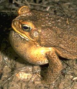
Repeated MeasuresIn an honours thesis from (1992), Mullens was investigating the ways that cane toads ( Bufo marinus ) respond to conditions of hypoxia. Toads show two different kinds of breathing patterns, lung or buccal, requiring them to be treated separately in the experiment. Her aim was to expose toads to a range of O2 concentrations, and record their breathing patterns, including parameters such as the expired volume for individual breaths. It was desirable to have around 8 replicates to compare the responses of the two breathing types, and the complication is that animals are expensive, and different individuals are likely to have different O2 profiles (leading to possibly reduced power). There are two main design options for this experiment;
- One animal per O2 treatment, 8 concentrations, 2 breathing types. With 8 replicates the experiment would require 128 animals, but that this could be analysed as a completely randomized design
- One O2 profile per animal, so that each animal would be used 8 times and only 16 animals are required (8 lung and 8 buccal breathers)
| Format of mullens.csv data file | |||||||||||||||||||||||||||||||||||||||||
|---|---|---|---|---|---|---|---|---|---|---|---|---|---|---|---|---|---|---|---|---|---|---|---|---|---|---|---|---|---|---|---|---|---|---|---|---|---|---|---|---|---|
|
 |
mullens <- read.table('../downloads/data/mullens.csv', header=T, sep=',', strip.white=T)
head(mullens)
  BREATH TOAD O2LEVEL FREQBUC SFREQBUC
1   lung    a       0    10.6    3.256
2   lung    a       5    18.8    4.336
3   lung    a      10    17.4    4.171
4   lung    a      15    16.6    4.074
5   lung    a      20     9.4    3.066
6   lung    a      30    11.4    3.376
Notice that the BREATH variable contains a categorical listing of the breathing type and that the first entries begin with "l" with comes after "b" in the alphabet (and therefore when BREATH is converted into a numeric, the first entry will be a 2. So we need to be careful that our codes reflect the order of the data.
Exploratory data analysis indicated that a square-root transformation of the FREQBUC (response variable) could normalize this variable and thereby address heterogeneity issues. Consequently, we too will apply a square-root transformation.
- Fit the JAGS model for the Randomized Complete Block
- Effects parameterization - random intercepts JAGS model
number of lesionsi = βSite j(i) + εi where ε ∼ N(0,σ2)
View full coderunif(1)
[1] 0.5659
modelString=


## write the model to a text file (I suggest you alter the path to somewhere more relevant
## to your system!)
writeLines(modelString,con="../downloads/BUGSscripts/ws9.4bQ4.1a.txt")


#sort the data set so that the breath treatments are in a more logical order
mullens.sort <- mullens[order(mullens$BREATH),]
mullens.sort$BREATH <- factor(mullens.sort$BREATH, levels = c("buccal", "lung"))
mullens.sort$TOAD <- factor(mullens.sort$TOAD, levels=unique(mullens.sort$TOAD))
br <- with(mullens.sort,BREATH[match(unique(TOAD),TOAD)])
br <- factor(br, levels=c("buccal", "lung"))
mullens.list <- with(mullens.sort,
                         list(freqbuc=FREQBUC,
                           o2level=as.numeric(O2LEVEL),
               cO2level=as.numeric(as.factor(O2LEVEL)),
               toad=as.numeric(TOAD),
                           br=factor(as.numeric(br)),
               breath=as.numeric(BREATH),
                           nO2level=length(levels(as.factor(O2LEVEL))),
                           nToad=length(levels(as.factor(TOAD))),
                           nBreath=length(levels(br)),
                           n=nrow(mullens.sort)
                           )
                           )
params <- c(
                  "g0","gamma.breath",
                  "beta.toad",
          "beta.o2level",
                  "beta.BreathO2level",
                  "Breath.means","O2level.means","BreathO2level.means",
                  "sd.O2level","sd.Breath","sd.Toad","sd.Resid","sd.BreathO2level",
                  "sigma.res","sigma.toad","sigma.breath","sigma.o2level","sigma.breatho2level"
                  )
adaptSteps = 1000
burnInSteps = 2000
nChains = 3
numSavedSteps = 5000
thinSteps = 10
nIter = ceiling((numSavedSteps * thinSteps)/nChains)

library(R2jags)
##
mullens.r2jags.a <- jags(data=mullens.list,
                                 inits=NULL, # since there are three chains
          parameters.to.save=params,
          model.file="../downloads/BUGSscripts/ws9.4bQ4.1a.txt",
          n.chains=3,
          n.iter=nIter,
          n.burnin=burnInSteps,
      n.thin=thinSteps
          )
Compiling data graph
   Resolving undeclared variables
   Allocating nodes
   Initializing
   Reading data back into data table
Compiling model graph
   Resolving undeclared variables
   Allocating nodes
   Graph Size: 1252

Initializing model
print(mullens.r2jags.a)
Inference for Bugs model at "../downloads/BUGSscripts/ws9.4bQ4.1a.txt", fit using jags, 3 chains, each with 16667 iterations (first 2000 discarded), n.thin = 10 n.sims = 4401 iterations saved mu.vect sd.vect 2.5% 25% 50% 75% 97.5% Rhat n.eff Breath.means[1] 4.937 0.357 4.213 4.699 4.940 5.181 5.625 1.001 3500 Breath.means[2] 1.541 0.463 0.645 1.236 1.539 1.851 2.436 1.001 4400 BreathO2level.means[1,1] 4.937 0.357 4.213 4.699 4.940 5.181 5.625 1.001 3500 BreathO2level.means[2,1] 1.541 0.463 0.645 1.236 1.539 1.851 2.436 1.001 4400 BreathO2level.means[1,2] 4.510 0.364 3.778 4.265 4.513 4.755 5.228 1.001 4400 BreathO2level.means[2,2] 2.555 0.474 1.614 2.240 2.555 2.869 3.472 1.001 4400 BreathO2level.means[1,3] 4.297 0.351 3.582 4.067 4.302 4.530 4.989 1.001 3600 BreathO2level.means[2,3] 3.367 0.460 2.463 3.056 3.372 3.671 4.255 1.001 4400 BreathO2level.means[1,4] 4.004 0.352 3.307 3.772 4.011 4.236 4.694 1.001 4400 BreathO2level.means[2,4] 3.085 0.452 2.190 2.779 3.094 3.380 3.953 1.001 4400 BreathO2level.means[1,5] 3.446 0.352 2.751 3.208 3.446 3.679 4.146 1.001 4400 BreathO2level.means[2,5] 3.225 0.462 2.325 2.912 3.210 3.531 4.132 1.001 4400 BreathO2level.means[1,6] 3.500 0.348 2.805 3.268 3.499 3.725 4.192 1.001 4400 BreathO2level.means[2,6] 3.030 0.455 2.146 2.730 3.037 3.335 3.905 1.001 4400 BreathO2level.means[1,7] 2.818 0.357 2.136 2.583 2.820 3.051 3.524 1.001 4400 BreathO2level.means[2,7] 2.817 0.460 1.900 2.509 2.819 3.117 3.739 1.001 4400 BreathO2level.means[1,8] 2.614 0.350 1.931 2.382 2.617 2.848 3.298 1.001 3300 BreathO2level.means[2,8] 2.461 0.465 1.529 2.162 2.453 2.777 3.363 1.001 4400 O2level.means[1] 3.650 0.189 3.270 3.525 3.652 3.778 4.023 1.001 4400 O2level.means[2] 3.223 0.294 2.653 3.025 3.220 3.424 3.778 1.002 1400 O2level.means[3] 3.010 0.275 2.471 2.822 3.010 3.194 3.544 1.001 4400 O2level.means[4] 2.717 0.273 2.179 2.535 2.717 2.900 3.262 1.001 3000 O2level.means[5] 2.159 0.277 1.629 1.967 2.161 2.346 2.696 1.002 2200 O2level.means[6] 2.213 0.275 1.668 2.030 2.216 2.393 2.739 1.001 4400 O2level.means[7] 1.531 0.280 0.989 1.341 1.529 1.725 2.080 1.002 1600 O2level.means[8] 1.327 0.280 0.775 1.140 1.330 1.518 1.873 1.001 2700 beta.BreathO2level[1,1] 0.000 0.000 0.000 0.000 0.000 0.000 0.000 1.000 1 beta.BreathO2level[2,1] 0.000 0.000 0.000 0.000 0.000 0.000 0.000 1.000 1 beta.BreathO2level[1,2] 0.000 0.000 0.000 0.000 0.000 0.000 0.000 1.000 1 beta.BreathO2level[2,2] 1.441 0.574 0.323 1.059 1.438 1.825 2.580 1.001 2500 beta.BreathO2level[1,3] 0.000 0.000 0.000 0.000 0.000 0.000 0.000 1.000 1 beta.BreathO2level[2,3] 2.466 0.532 1.420 2.109 2.471 2.807 3.515 1.001 4400 beta.BreathO2level[1,4] 0.000 0.000 0.000 0.000 0.000 0.000 0.000 1.000 1 beta.BreathO2level[2,4] 2.477 0.534 1.438 2.111 2.477 2.855 3.484 1.001 3400 beta.BreathO2level[1,5] 0.000 0.000 0.000 0.000 0.000 0.000 0.000 1.000 1 beta.BreathO2level[2,5] 3.176 0.533 2.130 2.812 3.179 3.543 4.211 1.002 1900 beta.BreathO2level[1,6] 0.000 0.000 0.000 0.000 0.000 0.000 0.000 1.000 1 beta.BreathO2level[2,6] 2.927 0.530 1.880 2.574 2.926 3.283 3.972 1.001 3500 beta.BreathO2level[1,7] 0.000 0.000 0.000 0.000 0.000 0.000 0.000 1.000 1 beta.BreathO2level[2,7] 3.396 0.542 2.340 3.038 3.391 3.757 4.468 1.001 3600 beta.BreathO2level[1,8] 0.000 0.000 0.000 0.000 0.000 0.000 0.000 1.000 1 beta.BreathO2level[2,8] 3.243 0.545 2.205 2.861 3.247 3.607 4.308 1.001 2400 beta.o2level[1] 0.000 0.000 0.000 0.000 0.000 0.000 0.000 1.000 1 beta.o2level[2] -0.427 0.355 -1.111 -0.668 -0.433 -0.187 0.278 1.002 2000 beta.o2level[3] -0.640 0.340 -1.292 -0.874 -0.646 -0.419 0.040 1.001 4400 beta.o2level[4] -0.934 0.334 -1.582 -1.159 -0.931 -0.706 -0.291 1.001 2900 beta.o2level[5] -1.492 0.337 -2.138 -1.723 -1.494 -1.267 -0.824 1.001 3100 beta.o2level[6] -1.438 0.333 -2.089 -1.663 -1.438 -1.217 -0.791 1.001 4400 beta.o2level[7] -2.120 0.339 -2.768 -2.345 -2.126 -1.893 -1.439 1.002 1600 beta.o2level[8] -2.324 0.340 -2.988 -2.557 -2.319 -2.092 -1.674 1.002 2200 beta.toad[1] 4.299 0.373 3.570 4.051 4.301 4.549 5.024 1.001 3200 beta.toad[2] 6.297 0.373 5.572 6.047 6.305 6.546 7.014 1.001 4400 beta.toad[3] 4.709 0.376 3.949 4.459 4.706 4.965 5.460 1.001 2900 beta.toad[4] 4.387 0.368 3.656 4.141 4.387 4.631 5.116 1.001 3300 beta.toad[5] 6.372 0.383 5.609 6.119 6.379 6.630 7.113 1.001 4400 beta.toad[6] 4.146 0.376 3.408 3.890 4.155 4.402 4.874 1.001 3400 beta.toad[7] 3.709 0.379 2.968 3.462 3.705 3.957 4.442 1.001 4400 beta.toad[8] 4.447 0.373 3.699 4.198 4.448 4.696 5.173 1.001 3000 beta.toad[9] 5.965 0.374 5.226 5.715 5.966 6.212 6.691 1.001 4400 beta.toad[10] 4.845 0.369 4.126 4.601 4.845 5.088 5.580 1.002 1700 beta.toad[11] 4.973 0.371 4.221 4.729 4.977 5.228 5.686 1.001 4400 beta.toad[12] 5.628 0.375 4.900 5.375 5.625 5.884 6.380 1.001 3900 beta.toad[13] 4.479 0.373 3.751 4.224 4.480 4.721 5.218 1.001 2600 beta.toad[14] 1.985 0.413 1.177 1.709 1.986 2.256 2.792 1.001 3700 beta.toad[15] 2.826 0.419 2.017 2.542 2.829 3.112 3.657 1.001 3500 beta.toad[16] 1.296 0.410 0.500 1.025 1.297 1.570 2.097 1.001 3300 beta.toad[17] 0.970 0.406 0.154 0.700 0.970 1.248 1.744 1.001 4400 beta.toad[18] 0.285 0.418 -0.532 0.004 0.289 0.560 1.084 1.001 4400 beta.toad[19] 2.189 0.413 1.375 1.909 2.194 2.465 2.993 1.001 4400 beta.toad[20] 1.590 0.418 0.772 1.310 1.587 1.870 2.406 1.001 4400 beta.toad[21] 1.259 0.411 0.451 0.992 1.251 1.539 2.061 1.001 3100 g0 4.937 0.357 4.213 4.699 4.940 5.181 5.625 1.001 3500 gamma.breath[1] 0.000 0.000 0.000 0.000 0.000 0.000 0.000 1.000 1 gamma.breath[2] -3.396 0.589 -4.548 -3.790 -3.399 -3.007 -2.237 1.001 4400 sd.Breath 2.402 0.416 1.582 2.126 2.404 2.680 3.216 1.001 4400 sd.BreathO2level 1.483 0.206 1.080 1.344 1.486 1.621 1.889 1.002 2000 sd.O2level 0.844 0.096 0.662 0.780 0.845 0.908 1.031 1.002 2100 sd.Resid 1.483 0.000 1.483 1.483 1.483 1.483 1.483 1.000 1 sd.Toad 0.883 0.083 0.729 0.828 0.880 0.934 1.057 1.002 1400 sigma.breath 49.572 28.985 2.350 24.101 49.438 74.781 97.415 1.001 4400 sigma.breatho2level 0.979 0.517 0.366 0.663 0.875 1.166 2.224 1.001 4400 sigma.o2level 0.969 0.430 0.465 0.695 0.868 1.123 2.018 1.001 3500 sigma.res 0.881 0.056 0.779 0.842 0.878 0.916 1.000 1.001 4400 sigma.toad 0.944 0.188 0.650 0.811 0.920 1.050 1.369 1.001 4400 deviance 432.451 10.234 414.872 425.254 431.611 438.804 454.837 1.001 4400 For each parameter, n.eff is a crude measure of effective sample size, and Rhat is the potential scale reduction factor (at convergence, Rhat=1). DIC info (using the rule, pD = var(deviance)/2) pD = 52.4 and DIC = 484.8 DIC is an estimate of expected predictive error (lower deviance is better). - Matrix parameterization - random intercepts model (JAGS)
number of lesionsi = βSite j(i) + εi where ε ∼ N(0,σ2)treating Distance as a factor
View full codeWe can perform generate the finite-population standard deviation posteriors within RmodelString=" model { #Likelihood for (i in 1:n) { y[i]~dnorm(mu[i],tau.res) mu[i] <- inprod(beta[],X[i,]) + inprod(gamma[],Z[i,]) y.err[i] <- y[i] - mu[1] } #Priors and derivatives for (i in 1:nZ) { gamma[i] ~ dnorm(0,tau.toad) } for (i in 1:nX) { beta[i] ~ dnorm(0,1.0E-06) } tau.res <- pow(sigma.res,-2) sigma.res <- z/sqrt(chSq) z ~ dnorm(0, .0016)I(0,) chSq ~ dgamma(0.5, 0.5) tau.toad <- pow(sigma.toad,-2) sigma.toad <- z.toad/sqrt(chSq.toad) z.toad ~ dnorm(0, .0016)I(0,) chSq.toad ~ dgamma(0.5, 0.5) } " ## write the model to a text file (I suggest you alter the path to somewhere more relevant ## to your system!) writeLines(modelString,con="../downloads/BUGSscripts/ws9.4bQ4.1b.txt") mullens$iO2LEVEL <- mullens$O2LEVEL mullens$O2LEVEL <- factor(mullens$O2LEVEL) Xmat <- model.matrix(~BREATH*O2LEVEL, data=mullens) Zmat <- model.matrix(~-1+TOAD, data=mullens) mullens.list <- list(y=mullens$SFREQBUC, X=Xmat, nX=ncol(Xmat), Z=Zmat, nZ=ncol(Zmat), n=nrow(mullens) ) params <- c("beta","gamma", "sigma.res","sigma.toad") burnInSteps = 3000 nChains = 3 numSavedSteps = 3000 thinSteps = 100 nIter = ceiling((numSavedSteps * thinSteps)/nChains) library(R2jags) library(coda) ## mullens.r2jags.b <- jags(data=mullens.list, inits=NULL, # since there are three chains parameters.to.save=params, model.file="../downloads/BUGSscripts/ws9.4bQ4.1b.txt", n.chains=3, n.iter=nIter, n.burnin=burnInSteps, n.thin=thinSteps )
Compiling model graph
   Resolving undeclared variables
   Allocating nodes
   Graph Size: 7073

Initializing model
print(mullens.r2jags.b)
Inference for Bugs model at "../downloads/BUGSscripts/ws9.4bQ4.1b.txt", fit using jags,
 3 chains, each with 1e+05 iterations (first 3000 discarded), n.thin = 100
 n.sims = 2910 iterations saved
           mu.vect sd.vect    2.5%     25%     50%     75%   97.5%  Rhat n.eff
beta[1]      4.948   0.359   4.258   4.707   4.943   5.186   5.655 1.001  2900
beta[2]     -3.405   0.571  -4.513  -3.784  -3.395  -3.035  -2.283 1.001  2900
beta[3]     -0.219   0.346  -0.910  -0.447  -0.219   0.019   0.466 1.001  2900
beta[4]     -0.549   0.349  -1.238  -0.783  -0.550  -0.315   0.143 1.001  2300
beta[5]     -0.868   0.348  -1.580  -1.105  -0.866  -0.628  -0.192 1.001  2900
beta[6]     -1.551   0.344  -2.226  -1.780  -1.549  -1.315  -0.886 1.001  2900
beta[7]     -1.472   0.351  -2.161  -1.703  -1.472  -1.240  -0.784 1.001  2900
beta[8]     -2.248   0.344  -2.920  -2.477  -2.248  -2.014  -1.585 1.001  2900
beta[9]     -2.466   0.344  -3.144  -2.701  -2.473  -2.226  -1.801 1.001  2900
beta[10]     1.050   0.545  -0.044   0.698   1.046   1.404   2.137 1.001  2400
beta[11]     2.337   0.550   1.257   1.968   2.340   2.721   3.440 1.002  1400
beta[12]     2.383   0.568   1.256   2.018   2.377   2.764   3.502 1.001  2900
beta[13]     3.307   0.552   2.221   2.950   3.297   3.672   4.382 1.001  2900
beta[14]     2.994   0.564   1.886   2.631   2.995   3.368   4.078 1.001  2900
beta[15]     3.637   0.559   2.573   3.263   3.635   4.014   4.724 1.001  2900
beta[16]     3.474   0.559   2.391   3.091   3.472   3.847   4.566 1.001  2900
gamma[1]     0.428   0.426  -0.370   0.146   0.425   0.705   1.270 1.001  2500
gamma[2]    -0.642   0.394  -1.442  -0.908  -0.641  -0.373   0.115 1.001  2900
gamma[3]     1.269   0.438   0.422   0.972   1.258   1.564   2.159 1.002  2600
gamma[4]     1.356   0.388   0.599   1.103   1.350   1.607   2.124 1.001  2900
gamma[5]    -0.253   0.392  -1.047  -0.506  -0.252   0.009   0.510 1.001  2900
gamma[6]    -0.551   0.392  -1.339  -0.814  -0.549  -0.282   0.196 1.001  2900
gamma[7]     1.419   0.399   0.640   1.149   1.418   1.685   2.202 1.001  2600
gamma[8]    -0.261   0.431  -1.119  -0.552  -0.256   0.036   0.561 1.001  2400
gamma[9]    -0.802   0.392  -1.554  -1.073  -0.802  -0.540  -0.031 1.001  2900
gamma[10]   -0.569   0.428  -1.415  -0.854  -0.563  -0.288   0.299 1.001  2900
gamma[11]   -1.253   0.391  -2.021  -1.510  -1.256  -0.984  -0.510 1.001  2200
gamma[12]   -0.489   0.384  -1.253  -0.752  -0.482  -0.225   0.250 1.002  1400
gamma[13]    1.010   0.397   0.219   0.741   1.012   1.265   1.807 1.001  2000
gamma[14]   -0.097   0.389  -0.868  -0.350  -0.096   0.165   0.650 1.000  2900
gamma[15]    0.029   0.379  -0.718  -0.224   0.028   0.289   0.772 1.001  2900
gamma[16]    0.677   0.381  -0.055   0.431   0.672   0.930   1.431 1.001  2900
gamma[17]   -1.261   0.437  -2.112  -1.559  -1.253  -0.964  -0.409 1.001  2900
gamma[18]   -0.464   0.386  -1.252  -0.713  -0.459  -0.205   0.286 1.001  2900
gamma[19]    0.642   0.430  -0.212   0.354   0.628   0.939   1.503 1.001  2900
gamma[20]    0.031   0.425  -0.817  -0.258   0.037   0.311   0.850 1.001  2900
gamma[21]   -0.281   0.434  -1.139  -0.573  -0.282  -0.012   0.611 1.001  2900
sigma.res    0.878   0.055   0.778   0.839   0.876   0.911   0.994 1.001  2900
sigma.toad   0.942   0.181   0.651   0.816   0.918   1.044   1.364 1.003   980
deviance   430.909   9.736 414.255 424.034 430.244 437.014 452.334 1.001  2900

For each parameter, n.eff is a crude measure of effective sample size,
and Rhat is the potential scale reduction factor (at convergence, Rhat=1).

DIC info (using the rule, pD = var(deviance)/2)
pD = 47.4 and DIC = 478.3
DIC is an estimate of expected predictive error (lower deviance is better).
mullens.mcmc.b <- as.mcmc(mullens.r2jags.b$BUGSoutput$sims.matrix)
View full codenms <- colnames(mullens.mcmc.b) pred <- grep('beta|gamma',nms) coefs <- mullens.mcmc.b[,pred] newdata <- mullens Amat <- cbind(model.matrix(~BREATH*O2LEVEL, newdata),model.matrix(~-1+TOAD, newdata)) pred <- coefs %*% t(Amat) y.err <- t(mullens$SFREQBUC - t(pred)) a<-apply(y.err, 1,sd) resid.sd <- data.frame(Source='Resid',Median=median(a), HPDinterval(as.mcmc(a)), HPDinterval(as.mcmc(a), p=0.68)) ## Fixed effects nms <- colnames(mullens.mcmc.b) mullens.mcmc.b.beta <- mullens.mcmc.b[,grep('beta',nms)] head(mullens.mcmc.b.beta)
Markov Chain Monte Carlo (MCMC) output:
Start = 1
End = 7
Thinning interval = 1
     beta[1] beta[2]  beta[3] beta[4] beta[5] beta[6] beta[7] beta[8] beta[9] beta[10] beta[11]
[1,]   4.880  -2.496 -0.05343 -0.7481 -0.5869  -1.303  -1.188  -2.697  -2.321   0.2640    1.960
[2,]   5.575  -4.377 -0.49387 -1.1872 -1.1980  -1.767  -2.255  -2.606  -3.232   1.7431    2.340
[3,]   4.713  -1.960  0.30678 -0.2729 -0.4483  -1.553  -1.069  -2.218  -1.847  -0.4305    1.920
[4,]   5.033  -3.070 -0.14523 -0.7453 -1.2370  -1.618  -1.541  -2.823  -2.764   0.5399    2.561
[5,]   5.207  -3.984 -0.31369 -0.3434 -0.8370  -1.739  -1.573  -2.461  -2.709   1.2610    2.792
[6,]   5.140  -3.714 -0.21333 -0.5883 -0.8169  -1.614  -1.250  -2.626  -2.566   1.5681    2.016
[7,]   5.242  -4.462 -0.20462 -0.9067 -0.4907  -1.488  -1.122  -2.258  -1.868   1.8402    3.712
     beta[12] beta[13] beta[14] beta[15] beta[16]
[1,]    2.088    2.270    2.255    3.151    2.693
[2,]    2.700    3.605    3.430    4.048    4.091
[3,]    1.969    2.808    1.580    2.820    2.129
[4,]    2.366    3.150    2.363    3.480    3.118
[5,]    2.947    3.921    2.883    3.865    3.885
[6,]    2.056    3.228    2.589    4.363    2.790
[7,]    2.583    3.699    3.751    4.453    3.467
assign <- attr(Xmat, 'assign') assign
[1] 0 1 2 2 2 2 2 2 2 3 3 3 3 3 3 3
nms <- attr(terms(model.frame(~BREATH*O2LEVEL, mullens)),'term.labels')
nms
[1] "BREATH" "O2LEVEL" "BREATH:O2LEVEL"
fixed.sd <- NULL
for (i in 1:max(assign)) {
   w <- which(i==assign)
   if (length(w)==1) fixed.sd<-cbind(fixed.sd, abs(mullens.mcmc.b.beta[,w])*sd(Xmat[,w]))
   else fixed.sd<-cbind(fixed.sd, apply(mullens.mcmc.b.beta[,w],1,sd))
}
library(plyr)
fixed.sd <-adply(fixed.sd,2,function(x) {
   data.frame(Median=median(x), HPDinterval(as.mcmc(x)), HPDinterval(as.mcmc(x), p=0.68))
})
fixed.sd<- cbind(Source=nms, fixed.sd)

# Variances
nms <- colnames(mullens.mcmc.b)
mullens.mcmc.b.gamma <- mullens.mcmc.b[,grep('gamma',nms)]
assign <- attr(Zmat, 'assign')
nms <- attr(terms(model.frame(~-1+TOAD, mullens)),'term.labels')
random.sd <- NULL
for (i in 1:max(assign)) {
   w <- which(i==assign)
   random.sd<-cbind(random.sd, apply(mullens.mcmc.b.gamma[,w],1,sd))
}
library(plyr)
random.sd <-adply(random.sd,2,function(x) {
   data.frame(Median=median(x), HPDinterval(as.mcmc(x)), HPDinterval(as.mcmc(x), p=0.68))
})
random.sd<- cbind(Source=nms, random.sd)

(mullens.sd <- rbind(subset(fixed.sd, select=-X1), subset(random.sd, select=-X1), resid.sd))
             Source Median  lower  upper lower.1 upper.1
1            BREATH 1.6535 1.1304 2.2066  1.3990  1.9352
2           O2LEVEL 0.8735 0.6746 1.0620  0.7710  0.9664
3    BREATH:O2LEVEL 0.9666 0.6726 1.2668  0.8278  1.1344
4              TOAD 0.8775 0.7264 1.0527  0.8048  0.9575
var1          Resid 0.8679 0.8246 0.9183  0.8400  0.8875
- Matrix parameterization - random intercepts model (STAN)
View full coderstanString=" data{ int n; int nZ; int nX; vector [n] y; matrix [n,nX] X; matrix [n,nZ] Z; vector [nX] a0; matrix [nX,nX] A0; } parameters{ vector [nX] beta; real<lower=0> sigma; vector [nZ] gamma; real<lower=0> sigma_Z; } transformed parameters { vector [n] mu; mu <- X*beta + Z*gamma; } model{ // Priors beta ~ multi_normal(a0,A0); gamma ~ normal( 0 , sigma_Z ); sigma_Z ~ cauchy(0,25); sigma ~ cauchy(0,25); y ~ normal( mu , sigma ); } generated quantities { vector [n] y_err; real<lower=0> sd_Resid; y_err <- y - mu; sd_Resid <- sd(y_err); } " #sort the data set so that the copper treatments are in a more logical order library(dplyr) mullens$O2LEVEL <- factor(mullens$O2LEVEL) Xmat <- model.matrix(~BREATH*O2LEVEL, data=mullens) Zmat <- model.matrix(~-1+TOAD, data=mullens) mullens.list <- list(y=mullens$SFREQBUC, X=Xmat, nX=ncol(Xmat), Z=Zmat, nZ=ncol(Zmat), n=nrow(mullens), a0=rep(0,ncol(Xmat)), A0=diag(100000,ncol(Xmat)) ) params <- c("beta","gamma", "sigma","sigma_Z") burnInSteps = 3000 nChains = 3 numSavedSteps = 3000 thinSteps = 10 nIter = ceiling((numSavedSteps * thinSteps)/nChains) library(rstan) library(coda) ## mullens.rstan.a <- stan(data=mullens.list, model_code=rstanString, pars=c("beta","gamma","sigma","sigma_Z"), chains=nChains, iter=nIter, warmup=burnInSteps, thin=thinSteps, save_dso=TRUE )
TRANSLATING MODEL 'rstanString' FROM Stan CODE TO C++ CODE NOW.
COMPILING THE C++ CODE FOR MODEL 'rstanString' NOW.

SAMPLING FOR MODEL 'rstanString' NOW (CHAIN 1).

Iteration:    1 / 10000 [  0%]  (Warmup)
Iteration: 1000 / 10000 [ 10%]  (Warmup)
Iteration: 2000 / 10000 [ 20%]  (Warmup)
Iteration: 3000 / 10000 [ 30%]  (Warmup)
Iteration: 3001 / 10000 [ 30%]  (Sampling)
Iteration: 4000 / 10000 [ 40%]  (Sampling)
Iteration: 5000 / 10000 [ 50%]  (Sampling)
Iteration: 6000 / 10000 [ 60%]  (Sampling)
Iteration: 7000 / 10000 [ 70%]  (Sampling)
Iteration: 8000 / 10000 [ 80%]  (Sampling)
Iteration: 9000 / 10000 [ 90%]  (Sampling)
Iteration: 10000 / 10000 [100%]  (Sampling)
#  Elapsed Time: 4.67 seconds (Warm-up)
#                13.17 seconds (Sampling)
#                17.84 seconds (Total)


SAMPLING FOR MODEL 'rstanString' NOW (CHAIN 2).

Iteration:    1 / 10000 [  0%]  (Warmup)
Iteration: 1000 / 10000 [ 10%]  (Warmup)
Iteration: 2000 / 10000 [ 20%]  (Warmup)
Iteration: 3000 / 10000 [ 30%]  (Warmup)
Iteration: 3001 / 10000 [ 30%]  (Sampling)
Iteration: 4000 / 10000 [ 40%]  (Sampling)
Iteration: 5000 / 10000 [ 50%]  (Sampling)
Iteration: 6000 / 10000 [ 60%]  (Sampling)
Iteration: 7000 / 10000 [ 70%]  (Sampling)
Iteration: 8000 / 10000 [ 80%]  (Sampling)
Iteration: 9000 / 10000 [ 90%]  (Sampling)
Iteration: 10000 / 10000 [100%]  (Sampling)
#  Elapsed Time: 4.56 seconds (Warm-up)
#                9.77 seconds (Sampling)
#                14.33 seconds (Total)


SAMPLING FOR MODEL 'rstanString' NOW (CHAIN 3).

Iteration:    1 / 10000 [  0%]  (Warmup)
Iteration: 1000 / 10000 [ 10%]  (Warmup)
Iteration: 2000 / 10000 [ 20%]  (Warmup)
Iteration: 3000 / 10000 [ 30%]  (Warmup)
Iteration: 3001 / 10000 [ 30%]  (Sampling)
Iteration: 4000 / 10000 [ 40%]  (Sampling)
Iteration: 5000 / 10000 [ 50%]  (Sampling)
Iteration: 6000 / 10000 [ 60%]  (Sampling)
Iteration: 7000 / 10000 [ 70%]  (Sampling)
Iteration: 8000 / 10000 [ 80%]  (Sampling)
Iteration: 9000 / 10000 [ 90%]  (Sampling)
Iteration: 10000 / 10000 [100%]  (Sampling)
#  Elapsed Time: 4.63 seconds (Warm-up)
#                15.57 seconds (Sampling)
#                20.2 seconds (Total)
print(mullens.rstan.a)
Inference for Stan model: rstanString.
3 chains, each with iter=10000; warmup=3000; thin=10;
post-warmup draws per chain=700, total post-warmup draws=2100.

            mean se_mean   sd   2.5%    25%    50%    75%  97.5% n_eff Rhat
beta[1]     4.94    0.01 0.36   4.23   4.70   4.94   5.18   5.62  1824    1
beta[2]    -3.40    0.01 0.57  -4.50  -3.79  -3.40  -3.02  -2.27  1878    1
beta[3]    -0.23    0.01 0.34  -0.89  -0.46  -0.23  -0.01   0.43  1814    1
beta[4]    -0.56    0.01 0.35  -1.22  -0.79  -0.56  -0.32   0.11  1956    1
beta[5]    -0.86    0.01 0.34  -1.52  -1.09  -0.87  -0.64  -0.18  1924    1
beta[6]    -1.55    0.01 0.34  -2.23  -1.78  -1.55  -1.32  -0.88  2100    1
beta[7]    -1.47    0.01 0.35  -2.13  -1.70  -1.46  -1.23  -0.79  2004    1
beta[8]    -2.26    0.01 0.34  -2.92  -2.47  -2.25  -2.03  -1.57  2041    1
beta[9]    -2.46    0.01 0.35  -3.11  -2.70  -2.46  -2.23  -1.78  1612    1
beta[10]    1.07    0.01 0.54   0.01   0.71   1.06   1.44   2.14  1856    1
beta[11]    2.35    0.01 0.55   1.28   1.97   2.35   2.74   3.46  1893    1
beta[12]    2.37    0.01 0.54   1.32   2.01   2.37   2.73   3.41  1989    1
beta[13]    3.31    0.01 0.54   2.27   2.93   3.31   3.69   4.39  2100    1
beta[14]    2.98    0.01 0.53   1.96   2.59   2.99   3.34   4.05  2100    1
beta[15]    3.64    0.01 0.55   2.54   3.25   3.63   4.01   4.70  2100    1
beta[16]    3.46    0.01 0.55   2.42   3.10   3.47   3.83   4.53  2100    1
gamma[1]    0.45    0.01 0.44  -0.39   0.16   0.45   0.74   1.29  1795    1
gamma[2]   -0.63    0.01 0.40  -1.46  -0.89  -0.64  -0.38   0.17  1540    1
gamma[3]    1.28    0.01 0.45   0.43   0.99   1.28   1.57   2.16  1806    1
gamma[4]    1.37    0.01 0.39   0.63   1.11   1.36   1.63   2.16  2094    1
gamma[5]   -0.22    0.01 0.39  -0.96  -0.49  -0.23   0.04   0.53  2003    1
gamma[6]   -0.54    0.01 0.39  -1.30  -0.80  -0.55  -0.28   0.23  1843    1
gamma[7]    1.43    0.01 0.38   0.67   1.17   1.43   1.68   2.16  2075    1
gamma[8]   -0.25    0.01 0.44  -1.10  -0.54  -0.24   0.04   0.62  2100    1
gamma[9]   -0.78    0.01 0.40  -1.58  -1.04  -0.77  -0.50  -0.02  1918    1
gamma[10]  -0.57    0.01 0.43  -1.44  -0.85  -0.57  -0.28   0.24  1888    1
gamma[11]  -1.23    0.01 0.38  -1.99  -1.48  -1.23  -0.97  -0.48  1878    1
gamma[12]  -0.48    0.01 0.38  -1.20  -0.74  -0.48  -0.21   0.26  1819    1
gamma[13]   1.02    0.01 0.40   0.27   0.76   1.02   1.29   1.81  1986    1
gamma[14]  -0.08    0.01 0.39  -0.84  -0.34  -0.07   0.17   0.64  1883    1
gamma[15]   0.03    0.01 0.38  -0.72  -0.23   0.03   0.29   0.82  1870    1
gamma[16]   0.68    0.01 0.39  -0.10   0.42   0.67   0.94   1.43  1861    1
gamma[17]  -1.25    0.01 0.45  -2.15  -1.54  -1.24  -0.95  -0.38  1987    1
gamma[18]  -0.45    0.01 0.39  -1.23  -0.69  -0.45  -0.19   0.29  1694    1
gamma[19]   0.65    0.01 0.45  -0.19   0.36   0.65   0.95   1.55  2011    1
gamma[20]   0.06    0.01 0.45  -0.81  -0.23   0.06   0.34   0.95  2042    1
gamma[21]  -0.28    0.01 0.43  -1.11  -0.56  -0.28   0.00   0.58  1975    1
sigma       0.88    0.00 0.05   0.78   0.84   0.88   0.91   1.00  2100    1
sigma_Z     0.94    0.00 0.19   0.65   0.81   0.91   1.05   1.40  2100    1
lp__      -69.80    0.11 4.97 -80.69 -72.81 -69.40 -66.24 -61.43  2080    1

Samples were drawn using NUTS(diag_e) at Sat Jan 31 08:07:18 2015.
For each parameter, n_eff is a crude measure of effective sample size,
and Rhat is the potential scale reduction factor on split chains (at
convergence, Rhat=1).
mullens.mcmc.c <- rstan:::as.mcmc.list.stanfit(mullens.rstan.a) mullens.mcmc.df.c <- as.data.frame(extract(mullens.rstan.a))
- Effects parameterization - random intercepts JAGS model
- Before fully exploring the parameters, it is prudent to examine the convergence and mixing diagnostics.
Chose either any of the parameterizations (they should yield much the same) - although it is sometimes useful to explore the
different performances of effects vs matrix and JAGS vs STAN.
- Effects parameterization - random intercepts model (JAGS)
Full effects parameterization JAGS code
library(coda)
plot(as.mcmc(mullens.r2jags.a))


autocorr.diag(as.mcmc(mullens.r2jags.a))
beta.BreathO2level[1,1] beta.BreathO2level[1,2] beta.BreathO2level[1,3] Lag 0 NaN NaN NaN Lag 10 NaN NaN NaN Lag 50 NaN NaN NaN Lag 100 NaN NaN NaN Lag 500 NaN NaN NaN beta.BreathO2level[1,4] beta.BreathO2level[1,5] beta.BreathO2level[1,6] Lag 0 NaN NaN NaN Lag 10 NaN NaN NaN Lag 50 NaN NaN NaN Lag 100 NaN NaN NaN Lag 500 NaN NaN NaN beta.BreathO2level[1,7] beta.BreathO2level[1,8] beta.BreathO2level[2,1] Lag 0 NaN NaN NaN Lag 10 NaN NaN NaN Lag 50 NaN NaN NaN Lag 100 NaN NaN NaN Lag 500 NaN NaN NaN beta.BreathO2level[2,2] beta.BreathO2level[2,3] beta.BreathO2level[2,4] Lag 0 1.000000 1.0000000 1.000000 Lag 10 0.047119 0.0506250 0.034635 Lag 50 -0.009087 -0.0149736 -0.012821 Lag 100 0.024438 0.0015708 -0.003077 Lag 500 0.014037 0.0008682 0.002473 beta.BreathO2level[2,5] beta.BreathO2level[2,6] beta.BreathO2level[2,7] Lag 0 1.000000 1.000000 1.000000 Lag 10 0.033593 0.030292 0.005748 Lag 50 -0.015182 -0.001415 -0.013241 Lag 100 0.002849 -0.016698 0.005768 Lag 500 0.007223 0.032042 -0.004683 beta.BreathO2level[2,8] beta.o2level[1] beta.o2level[2] beta.o2level[3] beta.o2level[4] Lag 0 1.000000 NaN 1.000000 1.000000 1.000000 Lag 10 0.042863 NaN 0.027329 0.025569 0.010036 Lag 50 -0.019776 NaN -0.005901 -0.008194 0.005864 Lag 100 -0.005399 NaN 0.008269 -0.023168 -0.005180 Lag 500 -0.012152 NaN -0.001524 -0.027353 0.003771 beta.o2level[5] beta.o2level[6] beta.o2level[7] beta.o2level[8] beta.toad[1] beta.toad[10] Lag 0 1.000000 1.0000000 1.000000 1.000000 1.000000 1.00000 Lag 10 0.036928 0.0185535 0.003299 0.028334 -0.001593 0.04462 Lag 50 -0.004048 0.0182058 -0.003061 0.006838 -0.002019 0.01890 Lag 100 -0.016865 0.0005485 -0.006426 -0.008995 -0.009017 -0.03212 Lag 500 -0.010894 0.0238321 -0.016793 -0.015019 0.007171 0.02463 beta.toad[11] beta.toad[12] beta.toad[13] beta.toad[14] beta.toad[15] beta.toad[16] Lag 0 1.000000 1.000000 1.000000 1.000000 1.000000 1.000000 Lag 10 0.005842 0.006679 0.003305 0.015319 0.025592 0.026067 Lag 50 -0.019360 -0.021964 0.004889 0.006421 -0.005712 -0.027088 Lag 100 -0.013033 -0.022123 -0.004888 0.020450 0.013593 0.029467 Lag 500 0.012187 0.003450 -0.015666 0.001582 0.009586 -0.002531 beta.toad[17] beta.toad[18] beta.toad[19] beta.toad[2] beta.toad[20] beta.toad[21] Lag 0 1.0000000 1.00000 1.000000 1.000000 1.000000 1.000000 Lag 10 0.0111070 0.00820 0.008287 0.001731 0.009009 0.015540 Lag 50 -0.0227707 -0.02585 -0.026784 0.004356 -0.003178 -0.013557 Lag 100 0.0004194 0.01487 0.023727 -0.034820 0.026590 0.018269 Lag 500 0.0017732 0.01014 -0.011858 0.021306 0.030587 -0.001805 beta.toad[3] beta.toad[4] beta.toad[5] beta.toad[6] beta.toad[7] beta.toad[8] beta.toad[9] Lag 0 1.000000 1.000000 1.000000 1.0000000 1.000000 1.000000 1.0000000 Lag 10 0.026248 0.033520 -0.002853 0.0079326 0.048105 0.014745 0.0070251 Lag 50 -0.006224 -0.018632 0.011086 0.0111348 -0.008393 -0.009974 -0.0037923 Lag 100 -0.017695 0.007070 0.009695 0.0214383 0.002776 0.005192 -0.0038539 Lag 500 -0.001430 0.003278 -0.010758 -0.0003823 -0.010444 -0.003600 -0.0001833 Breath.means[1] Breath.means[2] BreathO2level.means[1,1] BreathO2level.means[1,2] Lag 0 1.000000 1.000000 1.000000 1.0000000 Lag 10 0.036582 0.005327 0.036582 -0.0007928 Lag 50 0.019244 -0.023967 0.019244 -0.0002232 Lag 100 -0.026899 -0.013783 -0.026899 -0.0243188 Lag 500 0.009972 0.017985 0.009972 -0.0250686 BreathO2level.means[1,3] BreathO2level.means[1,4] BreathO2level.means[1,5] Lag 0 1.000000 1.000000 1.000e+00 Lag 10 -0.002974 -0.008895 1.080e-02 Lag 50 -0.017006 -0.003659 1.012e-03 Lag 100 -0.011183 -0.011478 8.337e-05 Lag 500 -0.041421 -0.011624 -5.894e-03 BreathO2level.means[1,6] BreathO2level.means[1,7] BreathO2level.means[1,8] Lag 0 1.000000 1.000000 1.000000 Lag 10 -0.010967 -0.004226 0.012048 Lag 50 0.019231 0.003087 0.006620 Lag 100 -0.008105 -0.006261 0.002103 Lag 500 0.005958 -0.015027 -0.001489 BreathO2level.means[2,1] BreathO2level.means[2,2] BreathO2level.means[2,3] Lag 0 1.000000 1.000000 1.000000 Lag 10 0.005327 0.004105 -0.023403 Lag 50 -0.023967 -0.003962 -0.001983 Lag 100 -0.013783 0.007083 0.005475 Lag 500 0.017985 0.017439 0.026444 BreathO2level.means[2,4] BreathO2level.means[2,5] BreathO2level.means[2,6] Lag 0 1.0000000 1.000000 1.000000 Lag 10 0.0024557 0.006148 -0.022192 Lag 50 0.0024848 -0.003669 0.001344 Lag 100 0.0006627 0.001880 -0.002367 Lag 500 -0.0074827 0.003152 0.025256 BreathO2level.means[2,7] BreathO2level.means[2,8] deviance g0 gamma.breath[1] Lag 0 1.0000000 1.000000 1.00000 1.000000 NaN Lag 10 0.0052862 0.014475 -0.01540 0.036582 NaN Lag 50 0.0015778 -0.004027 0.02459 0.019244 NaN Lag 100 0.0048619 -0.028792 0.01528 -0.026899 NaN Lag 500 0.0008909 -0.019027 0.02504 0.009972 NaN gamma.breath[2] O2level.means[1] O2level.means[2] O2level.means[3] O2level.means[4] Lag 0 1.000000 1.000000 1.000000 1.000000 1.000000 Lag 10 0.020644 0.020517 0.022473 0.018342 -0.001684 Lag 50 0.003897 -0.016476 0.001874 -0.012485 -0.002128 Lag 100 -0.036547 0.013658 0.026012 -0.004398 0.003771 Lag 500 0.008770 0.004398 0.009155 -0.024276 -0.009611 O2level.means[5] O2level.means[6] O2level.means[7] O2level.means[8] sd.Breath Lag 0 1.000000 1.000000 1.000000 1.000000 1.000000 Lag 10 0.021182 0.008326 -0.011953 0.027630 0.020644 Lag 50 -0.005484 0.008244 -0.001709 0.011116 0.003897 Lag 100 -0.008919 -0.005162 0.008085 0.005539 -0.036547 Lag 500 -0.007931 0.031386 -0.009182 -0.027264 0.008770 sd.BreathO2level sd.O2level sd.Resid sd.Toad sigma.breath sigma.breatho2level Lag 0 1.000000 1.000000 1.0000 1.000000 1.000000 1.000000 Lag 10 0.044683 0.023225 0.2341 0.003958 0.037212 0.175480 Lag 50 -0.017903 0.004359 0.2440 0.016063 0.022793 0.005456 Lag 100 -0.002324 -0.008736 0.2556 -0.008825 -0.007311 -0.019007 Lag 500 0.006114 -0.005205 0.2381 0.002690 0.010779 -0.002027 sigma.o2level sigma.res sigma.toad Lag 0 1.000000 1.0000000 1.0000000 Lag 10 0.083060 0.0002203 -0.0109140 Lag 50 0.007404 -0.0080565 0.0241421 Lag 100 0.005133 0.0241417 -0.0097403 Lag 500 0.016259 0.0070571 -0.0002376raftery.diag(as.mcmc(mullens.r2jags.a))
[[1]]

Quantile (q) = 0.025
Accuracy (r) = +/- 0.005
Probability (s) = 0.95

You need a sample size of at least 3746 with these values of q, r and s

[[2]]

Quantile (q) = 0.025
Accuracy (r) = +/- 0.005
Probability (s) = 0.95

You need a sample size of at least 3746 with these values of q, r and s

[[3]]

Quantile (q) = 0.025
Accuracy (r) = +/- 0.005
Probability (s) = 0.95

You need a sample size of at least 3746 with these values of q, r and s
- Matrix parameterization - random intercepts model (JAGS)
Matrix parameterization JAGS code
library(coda)
plot(as.mcmc(mullens.r2jags.b))


autocorr.diag(as.mcmc(mullens.r2jags.b))
beta[1] beta[10] beta[11] beta[12] beta[13] beta[14] beta[15] beta[16] beta[2] Lag 0 1.000000 1.000000 1.00000 1.000000 1.000000 1.000000 1.000000 1.000000 1.000000 Lag 100 -0.009529 0.020223 -0.01507 -0.005496 0.007946 0.008634 -0.022852 0.019268 0.002062 Lag 500 -0.021294 -0.001715 -0.02737 -0.002556 -0.031182 0.032546 0.014163 0.005448 -0.016038 Lag 1000 -0.014413 -0.006683 -0.01883 -0.015051 0.011445 0.023777 -0.006589 -0.015876 -0.026373 Lag 5000 0.015900 -0.006645 -0.00128 0.021914 -0.005969 -0.018341 -0.019482 0.003436 0.014180 beta[3] beta[4] beta[5] beta[6] beta[7] beta[8] beta[9] deviance gamma[1] Lag 0 1.0000000 1.000000 1.000000 1.000000 1.000000 1.000000 1.000000 1.000000 1.000000 Lag 100 0.0177713 0.014628 0.023477 0.011826 0.011188 -0.006122 0.039054 -0.007053 0.008715 Lag 500 0.0005351 -0.016122 -0.003339 -0.047636 0.002797 -0.009193 0.016943 0.005741 -0.015718 Lag 1000 0.0103756 0.001527 0.004306 0.038051 0.021410 0.017733 0.002051 0.006209 -0.023921 Lag 5000 -0.0061523 -0.002581 -0.008062 -0.003869 0.012019 0.001681 0.017883 0.029000 0.010628 gamma[10] gamma[11] gamma[12] gamma[13] gamma[14] gamma[15] gamma[16] gamma[17] gamma[18] Lag 0 1.000000 1.00000 1.000000 1.000000 1.000000 1.000000 1.000000 1.0000000 1.000000 Lag 100 0.005849 -0.01002 -0.003408 -0.005112 -0.010012 0.003537 -0.029072 0.0004839 -0.027524 Lag 500 -0.006139 0.02423 -0.003666 -0.015927 -0.008195 0.011496 -0.014997 0.0003654 -0.018112 Lag 1000 -0.005874 -0.02346 0.012999 -0.008720 0.010156 -0.030790 0.004532 -0.0124708 -0.012201 Lag 5000 0.020177 0.03262 -0.011651 0.001316 -0.006537 -0.001419 -0.011827 -0.0303006 -0.006169 gamma[19] gamma[2] gamma[20] gamma[21] gamma[3] gamma[4] gamma[5] gamma[6] gamma[7] Lag 0 1.000000 1.000000 1.0000000 1.000000 1.000000 1.000000 1.000000 1.000000 1.000000 Lag 100 -0.031045 -0.025773 -0.0007922 0.001488 -0.007735 -0.047942 -0.003091 -0.002262 -0.013798 Lag 500 -0.033347 -0.013008 -0.0282856 -0.013552 -0.032657 -0.012294 0.014231 -0.006998 0.015697 Lag 1000 -0.013012 -0.013592 -0.0015750 -0.020833 -0.032480 -0.004777 -0.021094 -0.007831 -0.016426 Lag 5000 -0.001349 0.008919 0.0141712 0.028123 0.031898 0.013191 0.003711 -0.013612 0.002735 gamma[8] gamma[9] sigma.res sigma.toad Lag 0 1.000000 1.000000 1.000000 1.000000 Lag 100 0.014759 -0.003898 0.013504 0.018135 Lag 500 -0.015630 -0.012040 0.006071 -0.034862 Lag 1000 -0.012948 -0.028001 -0.021278 -0.008229 Lag 5000 0.003267 0.019840 0.028059 -0.002177raftery.diag(as.mcmc(mullens.r2jags.b))
[[1]]

Quantile (q) = 0.025
Accuracy (r) = +/- 0.005
Probability (s) = 0.95

You need a sample size of at least 3746 with these values of q, r and s

[[2]]

Quantile (q) = 0.025
Accuracy (r) = +/- 0.005
Probability (s) = 0.95

You need a sample size of at least 3746 with these values of q, r and s

[[3]]

Quantile (q) = 0.025
Accuracy (r) = +/- 0.005
Probability (s) = 0.95

You need a sample size of at least 3746 with these values of q, r and s
- Matrix parameterization - random intercepts model (STAN)
Matrix parameterization STAN code
library(coda)
plot(mullens.mcmc.c)


autocorr.diag(mullens.mcmc.c)
beta[1] beta[2] beta[3] beta[4] beta[5] beta[6] beta[7] beta[8] beta[9] Lag 0 1.000000 1.00000 1.000000 1.00000 1.000000 1.00000 1.000000 1.000000 1.000000 Lag 10 0.075323 0.05882 0.038002 0.02209 0.030796 -0.01069 0.019391 0.013870 0.022758 Lag 50 -0.013816 -0.04673 -0.009117 -0.01837 0.006764 -0.03159 -0.006329 -0.003814 0.003805 Lag 100 0.007330 0.02789 -0.013747 -0.01304 0.017891 -0.01109 -0.033803 0.006073 -0.013934 Lag 500 0.002964 -0.01910 -0.009464 0.03431 0.046690 -0.02060 0.009052 0.036231 -0.015621 beta[10] beta[11] beta[12] beta[13] beta[14] beta[15] beta[16] gamma[1] gamma[2] Lag 0 1.00000 1.000000 1.00000 1.000000 1.000000 1.000000 1.000000 1.000000 1.000000 Lag 10 0.02094 0.021178 0.01595 -0.014799 -0.011231 -0.007213 -0.017970 0.003187 0.041076 Lag 50 -0.01304 -0.005547 0.01283 -0.042134 -0.021393 -0.023010 -0.004467 -0.008687 0.016969 Lag 100 0.03751 -0.012920 -0.01418 0.002542 0.012572 0.012367 0.002395 -0.018293 -0.009459 Lag 500 -0.02503 0.015152 0.01160 0.017864 -0.009359 0.044098 -0.002677 -0.043487 0.010978 gamma[3] gamma[4] gamma[5] gamma[6] gamma[7] gamma[8] gamma[9] gamma[10] gamma[11] Lag 0 1.000000 1.000000 1.000000 1.0000000 1.000000 1.000000 1.000000 1.000000 1.000000 Lag 10 0.031684 0.003337 0.014156 0.0309748 0.004975 -0.001067 0.047593 0.025183 0.048205 Lag 50 -0.009988 0.002532 0.022725 -0.0123910 0.009996 -0.063657 -0.006269 -0.022206 0.023040 Lag 100 -0.010721 0.005699 -0.008436 0.0054938 0.013723 0.013245 0.016127 0.004204 -0.003023 Lag 500 -0.029727 0.017845 -0.011151 -0.0007758 0.029995 -0.018522 0.012526 0.002633 0.024268 gamma[12] gamma[13] gamma[14] gamma[15] gamma[16] gamma[17] gamma[18] gamma[19] gamma[20] Lag 0 1.000000 1.000000 1.000000 1.000000 1.000000 1.000000 1.000000 1.000000 1.000000 Lag 10 0.066862 0.019748 0.058467 0.028520 0.065383 0.028599 0.066035 0.017727 0.012536 Lag 50 -0.011024 -0.010280 0.001222 -0.018740 0.009927 0.009400 0.006587 0.004028 -0.003746 Lag 100 -0.002287 0.048915 -0.020575 0.027193 -0.014911 -0.005238 -0.027403 -0.005643 -0.031967 Lag 500 0.002627 -0.001318 0.023401 0.004948 -0.023742 -0.009744 0.020779 -0.026538 -0.004190 gamma[21] sigma sigma_Z lp__ Lag 0 1.00000 1.00000 1.000000 1.000000 Lag 10 0.02849 -0.01214 -0.013233 0.001738 Lag 50 -0.01725 -0.03108 0.009673 -0.015617 Lag 100 -0.04150 -0.02959 -0.015358 -0.024548 Lag 500 -0.02824 0.01531 0.018352 -0.004852raftery.diag(mullens.mcmc.c)
[[1]]

Quantile (q) = 0.025
Accuracy (r) = +/- 0.005
Probability (s) = 0.95

You need a sample size of at least 3746 with these values of q, r and s

[[2]]

Quantile (q) = 0.025
Accuracy (r) = +/- 0.005
Probability (s) = 0.95

You need a sample size of at least 3746 with these values of q, r and s

[[3]]

Quantile (q) = 0.025
Accuracy (r) = +/- 0.005
Probability (s) = 0.95

You need a sample size of at least 3746 with these values of q, r and s
- Effects parameterization - random intercepts model (JAGS)
- Explore the parameter estimates
Full effects parameterization JAGS code
library(R2jags)
print(mullens.r2jags.a)
Inference for Bugs model at "../downloads/BUGSscripts/ws9.4bQ4.1a.txt", fit using jags,
 3 chains, each with 16667 iterations (first 2000 discarded), n.thin = 10
 n.sims = 4401 iterations saved
                         mu.vect sd.vect    2.5%     25%     50%     75%   97.5%  Rhat n.eff
Breath.means[1]            4.937   0.357   4.213   4.699   4.940   5.181   5.625 1.001  3500
Breath.means[2]            1.541   0.463   0.645   1.236   1.539   1.851   2.436 1.001  4400
BreathO2level.means[1,1]   4.937   0.357   4.213   4.699   4.940   5.181   5.625 1.001  3500
BreathO2level.means[2,1]   1.541   0.463   0.645   1.236   1.539   1.851   2.436 1.001  4400
BreathO2level.means[1,2]   4.510   0.364   3.778   4.265   4.513   4.755   5.228 1.001  4400
BreathO2level.means[2,2]   2.555   0.474   1.614   2.240   2.555   2.869   3.472 1.001  4400
BreathO2level.means[1,3]   4.297   0.351   3.582   4.067   4.302   4.530   4.989 1.001  3600
BreathO2level.means[2,3]   3.367   0.460   2.463   3.056   3.372   3.671   4.255 1.001  4400
BreathO2level.means[1,4]   4.004   0.352   3.307   3.772   4.011   4.236   4.694 1.001  4400
BreathO2level.means[2,4]   3.085   0.452   2.190   2.779   3.094   3.380   3.953 1.001  4400
BreathO2level.means[1,5]   3.446   0.352   2.751   3.208   3.446   3.679   4.146 1.001  4400
BreathO2level.means[2,5]   3.225   0.462   2.325   2.912   3.210   3.531   4.132 1.001  4400
BreathO2level.means[1,6]   3.500   0.348   2.805   3.268   3.499   3.725   4.192 1.001  4400
BreathO2level.means[2,6]   3.030   0.455   2.146   2.730   3.037   3.335   3.905 1.001  4400
BreathO2level.means[1,7]   2.818   0.357   2.136   2.583   2.820   3.051   3.524 1.001  4400
BreathO2level.means[2,7]   2.817   0.460   1.900   2.509   2.819   3.117   3.739 1.001  4400
BreathO2level.means[1,8]   2.614   0.350   1.931   2.382   2.617   2.848   3.298 1.001  3300
BreathO2level.means[2,8]   2.461   0.465   1.529   2.162   2.453   2.777   3.363 1.001  4400
O2level.means[1]           3.650   0.189   3.270   3.525   3.652   3.778   4.023 1.001  4400
O2level.means[2]           3.223   0.294   2.653   3.025   3.220   3.424   3.778 1.002  1400
O2level.means[3]           3.010   0.275   2.471   2.822   3.010   3.194   3.544 1.001  4400
O2level.means[4]           2.717   0.273   2.179   2.535   2.717   2.900   3.262 1.001  3000
O2level.means[5]           2.159   0.277   1.629   1.967   2.161   2.346   2.696 1.002  2200
O2level.means[6]           2.213   0.275   1.668   2.030   2.216   2.393   2.739 1.001  4400
O2level.means[7]           1.531   0.280   0.989   1.341   1.529   1.725   2.080 1.002  1600
O2level.means[8]           1.327   0.280   0.775   1.140   1.330   1.518   1.873 1.001  2700
beta.BreathO2level[1,1]    0.000   0.000   0.000   0.000   0.000   0.000   0.000 1.000     1
beta.BreathO2level[2,1]    0.000   0.000   0.000   0.000   0.000   0.000   0.000 1.000     1
beta.BreathO2level[1,2]    0.000   0.000   0.000   0.000   0.000   0.000   0.000 1.000     1
beta.BreathO2level[2,2]    1.441   0.574   0.323   1.059   1.438   1.825   2.580 1.001  2500
beta.BreathO2level[1,3]    0.000   0.000   0.000   0.000   0.000   0.000   0.000 1.000     1
beta.BreathO2level[2,3]    2.466   0.532   1.420   2.109   2.471   2.807   3.515 1.001  4400
beta.BreathO2level[1,4]    0.000   0.000   0.000   0.000   0.000   0.000   0.000 1.000     1
beta.BreathO2level[2,4]    2.477   0.534   1.438   2.111   2.477   2.855   3.484 1.001  3400
beta.BreathO2level[1,5]    0.000   0.000   0.000   0.000   0.000   0.000   0.000 1.000     1
beta.BreathO2level[2,5]    3.176   0.533   2.130   2.812   3.179   3.543   4.211 1.002  1900
beta.BreathO2level[1,6]    0.000   0.000   0.000   0.000   0.000   0.000   0.000 1.000     1
beta.BreathO2level[2,6]    2.927   0.530   1.880   2.574   2.926   3.283   3.972 1.001  3500
beta.BreathO2level[1,7]    0.000   0.000   0.000   0.000   0.000   0.000   0.000 1.000     1
beta.BreathO2level[2,7]    3.396   0.542   2.340   3.038   3.391   3.757   4.468 1.001  3600
beta.BreathO2level[1,8]    0.000   0.000   0.000   0.000   0.000   0.000   0.000 1.000     1
beta.BreathO2level[2,8]    3.243   0.545   2.205   2.861   3.247   3.607   4.308 1.001  2400
beta.o2level[1]            0.000   0.000   0.000   0.000   0.000   0.000   0.000 1.000     1
beta.o2level[2]           -0.427   0.355  -1.111  -0.668  -0.433  -0.187   0.278 1.002  2000
beta.o2level[3]           -0.640   0.340  -1.292  -0.874  -0.646  -0.419   0.040 1.001  4400
beta.o2level[4]           -0.934   0.334  -1.582  -1.159  -0.931  -0.706  -0.291 1.001  2900
beta.o2level[5]           -1.492   0.337  -2.138  -1.723  -1.494  -1.267  -0.824 1.001  3100
beta.o2level[6]           -1.438   0.333  -2.089  -1.663  -1.438  -1.217  -0.791 1.001  4400
beta.o2level[7]           -2.120   0.339  -2.768  -2.345  -2.126  -1.893  -1.439 1.002  1600
beta.o2level[8]           -2.324   0.340  -2.988  -2.557  -2.319  -2.092  -1.674 1.002  2200
beta.toad[1]               4.299   0.373   3.570   4.051   4.301   4.549   5.024 1.001  3200
beta.toad[2]               6.297   0.373   5.572   6.047   6.305   6.546   7.014 1.001  4400
beta.toad[3]               4.709   0.376   3.949   4.459   4.706   4.965   5.460 1.001  2900
beta.toad[4]               4.387   0.368   3.656   4.141   4.387   4.631   5.116 1.001  3300
beta.toad[5]               6.372   0.383   5.609   6.119   6.379   6.630   7.113 1.001  4400
beta.toad[6]               4.146   0.376   3.408   3.890   4.155   4.402   4.874 1.001  3400
beta.toad[7]               3.709   0.379   2.968   3.462   3.705   3.957   4.442 1.001  4400
beta.toad[8]               4.447   0.373   3.699   4.198   4.448   4.696   5.173 1.001  3000
beta.toad[9]               5.965   0.374   5.226   5.715   5.966   6.212   6.691 1.001  4400
beta.toad[10]              4.845   0.369   4.126   4.601   4.845   5.088   5.580 1.002  1700
beta.toad[11]              4.973   0.371   4.221   4.729   4.977   5.228   5.686 1.001  4400
beta.toad[12]              5.628   0.375   4.900   5.375   5.625   5.884   6.380 1.001  3900
beta.toad[13]              4.479   0.373   3.751   4.224   4.480   4.721   5.218 1.001  2600
beta.toad[14]              1.985   0.413   1.177   1.709   1.986   2.256   2.792 1.001  3700
beta.toad[15]              2.826   0.419   2.017   2.542   2.829   3.112   3.657 1.001  3500
beta.toad[16]              1.296   0.410   0.500   1.025   1.297   1.570   2.097 1.001  3300
beta.toad[17]              0.970   0.406   0.154   0.700   0.970   1.248   1.744 1.001  4400
beta.toad[18]              0.285   0.418  -0.532   0.004   0.289   0.560   1.084 1.001  4400
beta.toad[19]              2.189   0.413   1.375   1.909   2.194   2.465   2.993 1.001  4400
beta.toad[20]              1.590   0.418   0.772   1.310   1.587   1.870   2.406 1.001  4400
beta.toad[21]              1.259   0.411   0.451   0.992   1.251   1.539   2.061 1.001  3100
g0                         4.937   0.357   4.213   4.699   4.940   5.181   5.625 1.001  3500
gamma.breath[1]            0.000   0.000   0.000   0.000   0.000   0.000   0.000 1.000     1
gamma.breath[2]           -3.396   0.589  -4.548  -3.790  -3.399  -3.007  -2.237 1.001  4400
sd.Breath                  2.402   0.416   1.582   2.126   2.404   2.680   3.216 1.001  4400
sd.BreathO2level           1.483   0.206   1.080   1.344   1.486   1.621   1.889 1.002  2000
sd.O2level                 0.844   0.096   0.662   0.780   0.845   0.908   1.031 1.002  2100
sd.Resid                   1.483   0.000   1.483   1.483   1.483   1.483   1.483 1.000     1
sd.Toad                    0.883   0.083   0.729   0.828   0.880   0.934   1.057 1.002  1400
sigma.breath              49.572  28.985   2.350  24.101  49.438  74.781  97.415 1.001  4400
sigma.breatho2level        0.979   0.517   0.366   0.663   0.875   1.166   2.224 1.001  4400
sigma.o2level              0.969   0.430   0.465   0.695   0.868   1.123   2.018 1.001  3500
sigma.res                  0.881   0.056   0.779   0.842   0.878   0.916   1.000 1.001  4400
sigma.toad                 0.944   0.188   0.650   0.811   0.920   1.050   1.369 1.001  4400
deviance                 432.451  10.234 414.872 425.254 431.611 438.804 454.837 1.001  4400

For each parameter, n.eff is a crude measure of effective sample size,
and Rhat is the potential scale reduction factor (at convergence, Rhat=1).

DIC info (using the rule, pD = var(deviance)/2)
pD = 52.4 and DIC = 484.8
DIC is an estimate of expected predictive error (lower deviance is better).
Matrix parameterization JAGS codelibrary(R2jags) print(mullens.r2jags.b)
Inference for Bugs model at "../downloads/BUGSscripts/ws9.4bQ4.1b.txt", fit using jags,
 3 chains, each with 1e+05 iterations (first 3000 discarded), n.thin = 100
 n.sims = 2910 iterations saved
           mu.vect sd.vect    2.5%     25%     50%     75%   97.5%  Rhat n.eff
beta[1]      4.948   0.359   4.258   4.707   4.943   5.186   5.655 1.001  2900
beta[2]     -3.405   0.571  -4.513  -3.784  -3.395  -3.035  -2.283 1.001  2900
beta[3]     -0.219   0.346  -0.910  -0.447  -0.219   0.019   0.466 1.001  2900
beta[4]     -0.549   0.349  -1.238  -0.783  -0.550  -0.315   0.143 1.001  2300
beta[5]     -0.868   0.348  -1.580  -1.105  -0.866  -0.628  -0.192 1.001  2900
beta[6]     -1.551   0.344  -2.226  -1.780  -1.549  -1.315  -0.886 1.001  2900
beta[7]     -1.472   0.351  -2.161  -1.703  -1.472  -1.240  -0.784 1.001  2900
beta[8]     -2.248   0.344  -2.920  -2.477  -2.248  -2.014  -1.585 1.001  2900
beta[9]     -2.466   0.344  -3.144  -2.701  -2.473  -2.226  -1.801 1.001  2900
beta[10]     1.050   0.545  -0.044   0.698   1.046   1.404   2.137 1.001  2400
beta[11]     2.337   0.550   1.257   1.968   2.340   2.721   3.440 1.002  1400
beta[12]     2.383   0.568   1.256   2.018   2.377   2.764   3.502 1.001  2900
beta[13]     3.307   0.552   2.221   2.950   3.297   3.672   4.382 1.001  2900
beta[14]     2.994   0.564   1.886   2.631   2.995   3.368   4.078 1.001  2900
beta[15]     3.637   0.559   2.573   3.263   3.635   4.014   4.724 1.001  2900
beta[16]     3.474   0.559   2.391   3.091   3.472   3.847   4.566 1.001  2900
gamma[1]     0.428   0.426  -0.370   0.146   0.425   0.705   1.270 1.001  2500
gamma[2]    -0.642   0.394  -1.442  -0.908  -0.641  -0.373   0.115 1.001  2900
gamma[3]     1.269   0.438   0.422   0.972   1.258   1.564   2.159 1.002  2600
gamma[4]     1.356   0.388   0.599   1.103   1.350   1.607   2.124 1.001  2900
gamma[5]    -0.253   0.392  -1.047  -0.506  -0.252   0.009   0.510 1.001  2900
gamma[6]    -0.551   0.392  -1.339  -0.814  -0.549  -0.282   0.196 1.001  2900
gamma[7]     1.419   0.399   0.640   1.149   1.418   1.685   2.202 1.001  2600
gamma[8]    -0.261   0.431  -1.119  -0.552  -0.256   0.036   0.561 1.001  2400
gamma[9]    -0.802   0.392  -1.554  -1.073  -0.802  -0.540  -0.031 1.001  2900
gamma[10]   -0.569   0.428  -1.415  -0.854  -0.563  -0.288   0.299 1.001  2900
gamma[11]   -1.253   0.391  -2.021  -1.510  -1.256  -0.984  -0.510 1.001  2200
gamma[12]   -0.489   0.384  -1.253  -0.752  -0.482  -0.225   0.250 1.002  1400
gamma[13]    1.010   0.397   0.219   0.741   1.012   1.265   1.807 1.001  2000
gamma[14]   -0.097   0.389  -0.868  -0.350  -0.096   0.165   0.650 1.000  2900
gamma[15]    0.029   0.379  -0.718  -0.224   0.028   0.289   0.772 1.001  2900
gamma[16]    0.677   0.381  -0.055   0.431   0.672   0.930   1.431 1.001  2900
gamma[17]   -1.261   0.437  -2.112  -1.559  -1.253  -0.964  -0.409 1.001  2900
gamma[18]   -0.464   0.386  -1.252  -0.713  -0.459  -0.205   0.286 1.001  2900
gamma[19]    0.642   0.430  -0.212   0.354   0.628   0.939   1.503 1.001  2900
gamma[20]    0.031   0.425  -0.817  -0.258   0.037   0.311   0.850 1.001  2900
gamma[21]   -0.281   0.434  -1.139  -0.573  -0.282  -0.012   0.611 1.001  2900
sigma.res    0.878   0.055   0.778   0.839   0.876   0.911   0.994 1.001  2900
sigma.toad   0.942   0.181   0.651   0.816   0.918   1.044   1.364 1.003   980
deviance   430.909   9.736 414.255 424.034 430.244 437.014 452.334 1.001  2900

For each parameter, n.eff is a crude measure of effective sample size,
and Rhat is the potential scale reduction factor (at convergence, Rhat=1).

DIC info (using the rule, pD = var(deviance)/2)
pD = 47.4 and DIC = 478.3
DIC is an estimate of expected predictive error (lower deviance is better).
Matrix parameterization STAN codelibrary(R2jags) print(mullens.rstan.a)
Inference for Stan model: rstanString. 3 chains, each with iter=10000; warmup=3000; thin=10; post-warmup draws per chain=700, total post-warmup draws=2100. mean se_mean sd 2.5% 25% 50% 75% 97.5% n_eff Rhat beta[1] 4.94 0.01 0.36 4.23 4.70 4.94 5.18 5.62 1824 1 beta[2] -3.40 0.01 0.57 -4.50 -3.79 -3.40 -3.02 -2.27 1878 1 beta[3] -0.23 0.01 0.34 -0.89 -0.46 -0.23 -0.01 0.43 1814 1 beta[4] -0.56 0.01 0.35 -1.22 -0.79 -0.56 -0.32 0.11 1956 1 beta[5] -0.86 0.01 0.34 -1.52 -1.09 -0.87 -0.64 -0.18 1924 1 beta[6] -1.55 0.01 0.34 -2.23 -1.78 -1.55 -1.32 -0.88 2100 1 beta[7] -1.47 0.01 0.35 -2.13 -1.70 -1.46 -1.23 -0.79 2004 1 beta[8] -2.26 0.01 0.34 -2.92 -2.47 -2.25 -2.03 -1.57 2041 1 beta[9] -2.46 0.01 0.35 -3.11 -2.70 -2.46 -2.23 -1.78 1612 1 beta[10] 1.07 0.01 0.54 0.01 0.71 1.06 1.44 2.14 1856 1 beta[11] 2.35 0.01 0.55 1.28 1.97 2.35 2.74 3.46 1893 1 beta[12] 2.37 0.01 0.54 1.32 2.01 2.37 2.73 3.41 1989 1 beta[13] 3.31 0.01 0.54 2.27 2.93 3.31 3.69 4.39 2100 1 beta[14] 2.98 0.01 0.53 1.96 2.59 2.99 3.34 4.05 2100 1 beta[15] 3.64 0.01 0.55 2.54 3.25 3.63 4.01 4.70 2100 1 beta[16] 3.46 0.01 0.55 2.42 3.10 3.47 3.83 4.53 2100 1 gamma[1] 0.45 0.01 0.44 -0.39 0.16 0.45 0.74 1.29 1795 1 gamma[2] -0.63 0.01 0.40 -1.46 -0.89 -0.64 -0.38 0.17 1540 1 gamma[3] 1.28 0.01 0.45 0.43 0.99 1.28 1.57 2.16 1806 1 gamma[4] 1.37 0.01 0.39 0.63 1.11 1.36 1.63 2.16 2094 1 gamma[5] -0.22 0.01 0.39 -0.96 -0.49 -0.23 0.04 0.53 2003 1 gamma[6] -0.54 0.01 0.39 -1.30 -0.80 -0.55 -0.28 0.23 1843 1 gamma[7] 1.43 0.01 0.38 0.67 1.17 1.43 1.68 2.16 2075 1 gamma[8] -0.25 0.01 0.44 -1.10 -0.54 -0.24 0.04 0.62 2100 1 gamma[9] -0.78 0.01 0.40 -1.58 -1.04 -0.77 -0.50 -0.02 1918 1 gamma[10] -0.57 0.01 0.43 -1.44 -0.85 -0.57 -0.28 0.24 1888 1 gamma[11] -1.23 0.01 0.38 -1.99 -1.48 -1.23 -0.97 -0.48 1878 1 gamma[12] -0.48 0.01 0.38 -1.20 -0.74 -0.48 -0.21 0.26 1819 1 gamma[13] 1.02 0.01 0.40 0.27 0.76 1.02 1.29 1.81 1986 1 gamma[14] -0.08 0.01 0.39 -0.84 -0.34 -0.07 0.17 0.64 1883 1 gamma[15] 0.03 0.01 0.38 -0.72 -0.23 0.03 0.29 0.82 1870 1 gamma[16] 0.68 0.01 0.39 -0.10 0.42 0.67 0.94 1.43 1861 1 gamma[17] -1.25 0.01 0.45 -2.15 -1.54 -1.24 -0.95 -0.38 1987 1 gamma[18] -0.45 0.01 0.39 -1.23 -0.69 -0.45 -0.19 0.29 1694 1 gamma[19] 0.65 0.01 0.45 -0.19 0.36 0.65 0.95 1.55 2011 1 gamma[20] 0.06 0.01 0.45 -0.81 -0.23 0.06 0.34 0.95 2042 1 gamma[21] -0.28 0.01 0.43 -1.11 -0.56 -0.28 0.00 0.58 1975 1 sigma 0.88 0.00 0.05 0.78 0.84 0.88 0.91 1.00 2100 1 sigma_Z 0.94 0.00 0.19 0.65 0.81 0.91 1.05 1.40 2100 1 lp__ -69.80 0.11 4.97 -80.69 -72.81 -69.40 -66.24 -61.43 2080 1 Samples were drawn using NUTS(diag_e) at Sat Jan 31 08:07:18 2015. For each parameter, n_eff is a crude measure of effective sample size, and Rhat is the potential scale reduction factor on split chains (at convergence, Rhat=1). - Figure time
Matrix parameterization JAGS code
nms <- colnames(mullens.mcmc.b)
pred <- grep('beta',nms)
coefs <- mullens.mcmc.b[,pred]
newdata <- expand.grid(BREATH=levels(mullens$BREATH), O2LEVEL=levels(mullens$O2LEVEL))
Xmat <- model.matrix(~BREATH*O2LEVEL, newdata)
pred <- coefs %*% t(Xmat)
library(plyr)
newdata <- cbind(newdata, adply(pred, 2, function(x) {
   data.frame(Median=median(x), HPDinterval(as.mcmc(x)), HPDinterval(as.mcmc(x), p=0.68))
}))
newdata
   BREATH O2LEVEL X1 Median  lower upper lower.1 upper.1
1  buccal       0  1  4.943 4.2389 5.618   4.561   5.269
2    lung       0  2  1.550 0.6998 2.466   1.132   2.001
3  buccal       5  3  4.728 4.0285 5.432   4.371   5.082
4    lung       5  4  2.375 1.5123 3.301   1.848   2.747
5  buccal      10  5  4.395 3.7066 5.086   4.007   4.726
6    lung      10  6  3.325 2.4879 4.218   2.871   3.765
7  buccal      15  7  4.085 3.3682 4.791   3.682   4.406
8    lung      15  8  3.059 2.1765 3.968   2.571   3.469
9  buccal      20  9  3.389 2.6788 4.076   3.011   3.718
10   lung      20 10  3.301 2.3525 4.161   2.842   3.722
11 buccal      30 11  3.480 2.7380 4.156   3.168   3.891
12   lung      30 12  3.066 2.1262 3.906   2.615   3.502
13 buccal      40 13  2.698 2.0185 3.435   2.332   3.018
14   lung      40 14  2.923 2.0682 3.855   2.511   3.384
15 buccal      50 15  2.470 1.7995 3.203   2.113   2.827
16   lung      50 16  2.548 1.7116 3.480   2.104   3.005
library(ggplot2)
p1 <-ggplot(newdata, aes(y=Median, x=as.integer(O2LEVEL), fill=BREATH)) +
  geom_line(aes(linetype=BREATH)) +
  #geom_line()+
  geom_linerange(aes(ymin=lower, ymax=upper), show_guide=FALSE)+
  geom_linerange(aes(ymin=lower.1, ymax=upper.1), size=2,show_guide=FALSE)+
  geom_point(size=3, shape=21)+
  scale_y_continuous(expression(Frequency~of~buccal~breathing))+
  scale_x_continuous('Oxygen concentration')+
  scale_fill_manual('Breath type', breaks=c('buccal','lung'), values=c('black','white'),
                    labels=c('Buccal','Lung'))+
  scale_linetype_manual('Breath type', breaks=c('buccal','lung'), values=c('solid','dashed'),
                    labels=c('Buccal','Lung'))+
  theme_classic() +
  theme(legend.justification=c(1,0), legend.position=c(1,0),
        legend.key.width=unit(3,'lines'),
        axis.title.y=element_text(vjust=2, size=rel(1.2)),
        axis.title.x=element_text(vjust=-1, size=rel(1.2)),
        plot.margin=unit(c(0.5,0.5,1,2),'lines'))

mullens.sd$Source <- factor(mullens.sd$Source, levels=c("Resid","BREATH:O2LEVEL","O2LEVEL","TOAD","BREATH"),
    labels=c("Residuals", "Breath:O2", "O2","Toad","Breath"))
mullens.sd$Perc <- 100*mullens.sd$Median/sum(mullens.sd$Median)

p2<-ggplot(mullens.sd,aes(y=Source, x=Median))+
  geom_vline(xintercept=0,linetype="dashed")+
  geom_hline(xintercept=0)+
  scale_x_continuous("Finite population \nvariance components (sd)")+
  geom_errorbarh(aes(xmin=lower.1, xmax=upper.1), height=0, size=1)+
  geom_errorbarh(aes(xmin=lower, xmax=upper), height=0, size=1.5)+
  geom_point(size=3)+
  geom_text(aes(label=sprintf("(%4.1f%%)",Perc),vjust=-1))+
  theme_classic()+
  theme(axis.line=element_blank(),axis.title.y=element_blank(),
       axis.text.y=element_text(size=12,hjust=1))

library(gridExtra)
grid.arrange(p1, p2, ncol=2)

- As an alternative, we could model oxygen concentration as a numeric...
Matrix parameterization JAGS codeWe can perform generate the finite-population standard deviation posteriors within R
modelString="
model {
   #Likelihood
   for (i in 1:n) {
      y[i]~dnorm(mu[i],tau.res)
      mu[i] <- inprod(beta[],X[i,]) + inprod(gamma[],Z[i,])
      y.err[i] <- y[i] - mu[1]
   }

   #Priors and derivatives
   for (i in 1:nZ) {
      gamma[i] ~ dnorm(0,tau.toad)
   }
   for (i in 1:nX) {
      beta[i] ~ dnorm(0,1.0E-06)
   }

   tau.res <- pow(sigma.res,-2)
   sigma.res <- z/sqrt(chSq)
   z ~ dnorm(0, .0016)I(0,)
   chSq ~ dgamma(0.5, 0.5)

   tau.toad <- pow(sigma.toad,-2)
   sigma.toad <- z.toad/sqrt(chSq.toad)
   z.toad ~ dnorm(0, .0016)I(0,)
   chSq.toad ~ dgamma(0.5, 0.5)

 }
"

## write the model to a text file (I suggest you alter the path to somewhere more relevant
## to your system!)
writeLines(modelString,con="../downloads/BUGSscripts/ws9.4bQ4.6a.txt")

Xmat <- model.matrix(~BREATH*iO2LEVEL, data=mullens)
Zmat <- model.matrix(~-1+TOAD, data=mullens)
mullens.list <- list(y=mullens$SFREQBUC,
               X=Xmat, nX=ncol(Xmat),
                           Z=Zmat, nZ=ncol(Zmat),
                           n=nrow(mullens)
                           )
params <- c("beta","gamma",
                  "sigma.res","sigma.toad")
burnInSteps = 3000
nChains = 3
numSavedSteps = 3000
thinSteps = 100
nIter = ceiling((numSavedSteps * thinSteps)/nChains)

library(R2jags)
library(coda)
##
mullens.r2jags.d <- jags(data=mullens.list,
                                 inits=NULL, # since there are three chains
          parameters.to.save=params,
          model.file="../downloads/BUGSscripts/ws9.4bQ4.6a.txt",
          n.chains=3,
          n.iter=nIter,
          n.burnin=burnInSteps,
      n.thin=thinSteps
          )
Compiling model graph
   Resolving undeclared variables
   Allocating nodes
   Graph Size: 5045

Initializing model
print(mullens.r2jags.d)
Inference for Bugs model at "../downloads/BUGSscripts/ws9.4bQ4.6a.txt", fit using jags,
 3 chains, each with 1e+05 iterations (first 3000 discarded), n.thin = 100
 n.sims = 2910 iterations saved
           mu.vect sd.vect    2.5%     25%     50%     75%   97.5%  Rhat n.eff
beta[1]      4.848   0.308   4.234   4.641   4.850   5.059   5.445 1.001  2900
beta[2]     -2.296   0.503  -3.254  -2.639  -2.288  -1.982  -1.287 1.001  2900
beta[3]     -0.051   0.006  -0.062  -0.054  -0.051  -0.047  -0.040 1.002  1900
beta[4]      0.062   0.009   0.043   0.055   0.062   0.067   0.080 1.003  1400
gamma[1]     0.417   0.445  -0.482   0.115   0.424   0.719   1.277 1.001  2900
gamma[2]    -0.636   0.397  -1.417  -0.895  -0.642  -0.369   0.130 1.001  2900
gamma[3]     1.252   0.449   0.365   0.957   1.244   1.548   2.158 1.001  2900
gamma[4]     1.342   0.402   0.573   1.075   1.336   1.602   2.170 1.001  2900
gamma[5]    -0.233   0.403  -1.034  -0.494  -0.229   0.038   0.558 1.001  2900
gamma[6]    -0.538   0.398  -1.297  -0.803  -0.543  -0.278   0.224 1.001  2900
gamma[7]     1.418   0.410   0.624   1.131   1.416   1.684   2.258 1.001  2900
gamma[8]    -0.272   0.439  -1.148  -0.568  -0.267   0.021   0.587 1.002  1100
gamma[9]    -0.778   0.398  -1.567  -1.040  -0.769  -0.513   0.000 1.001  2900
gamma[10]   -0.584   0.445  -1.473  -0.880  -0.585  -0.277   0.264 1.001  2200
gamma[11]   -1.226   0.403  -2.025  -1.504  -1.219  -0.949  -0.449 1.001  2900
gamma[12]   -0.487   0.392  -1.236  -0.758  -0.487  -0.221   0.270 1.001  2900
gamma[13]    1.012   0.399   0.253   0.747   1.000   1.270   1.802 1.001  2900
gamma[14]   -0.085   0.399  -0.875  -0.342  -0.083   0.185   0.717 1.001  2900
gamma[15]    0.031   0.396  -0.744  -0.232   0.030   0.289   0.810 1.001  2900
gamma[16]    0.673   0.403  -0.067   0.401   0.664   0.931   1.490 1.001  2900
gamma[17]   -1.263   0.456  -2.202  -1.568  -1.257  -0.952  -0.383 1.001  2900
gamma[18]   -0.457   0.404  -1.275  -0.728  -0.457  -0.186   0.322 1.001  2900
gamma[19]    0.624   0.443  -0.238   0.333   0.627   0.919   1.503 1.001  2900
gamma[20]    0.030   0.442  -0.849  -0.257   0.030   0.329   0.911 1.001  2900
gamma[21]   -0.295   0.448  -1.187  -0.593  -0.298   0.004   0.583 1.001  2900
sigma.res    0.925   0.054   0.824   0.888   0.922   0.961   1.038 1.002  1000
sigma.toad   0.938   0.188   0.638   0.804   0.919   1.046   1.366 1.001  2900
deviance   449.164   7.815 436.212 443.536 448.455 454.081 466.831 1.001  2900

For each parameter, n.eff is a crude measure of effective sample size,
and Rhat is the potential scale reduction factor (at convergence, Rhat=1).

DIC info (using the rule, pD = var(deviance)/2)
pD = 30.6 and DIC = 479.7
DIC is an estimate of expected predictive error (lower deviance is better).
mullens.mcmc.d <- as.mcmc(mullens.r2jags.d$BUGSoutput$sims.matrix)
View full codenms <- colnames(mullens.mcmc.d) pred <- grep('beta|gamma',nms) coefs <- mullens.mcmc.d[,pred] newdata <- mullens Amat <- cbind(model.matrix(~BREATH*iO2LEVEL, newdata),model.matrix(~-1+TOAD, newdata)) pred <- coefs %*% t(Amat) y.err <- t(mullens$SFREQBUC - t(pred)) a<-apply(y.err, 1,sd) resid.sd <- data.frame(Source='Resid',Median=median(a), HPDinterval(as.mcmc(a)), HPDinterval(as.mcmc(a), p=0.68)) ## Fixed effects nms <- colnames(mullens.mcmc.d) mullens.mcmc.d.beta <- mullens.mcmc.d[,grep('beta',nms)] head(mullens.mcmc.d.beta)
Markov Chain Monte Carlo (MCMC) output:
Start = 1
End = 7
Thinning interval = 1
     beta[1] beta[2]  beta[3] beta[4]
[1,]   4.674  -2.208 -0.05177 0.06361
[2,]   5.172  -2.802 -0.06305 0.06144
[3,]   5.563  -2.930 -0.06357 0.06296
[4,]   4.651  -2.148 -0.04643 0.05753
[5,]   5.183  -2.749 -0.05130 0.06486
[6,]   4.836  -1.440 -0.05132 0.06433
[7,]   4.938  -2.385 -0.04854 0.06522
assign <- attr(Xmat, 'assign') assign
[1] 0 1 2 3
nms <- attr(terms(model.frame(~BREATH*iO2LEVEL, mullens)),'term.labels')
nms
[1] "BREATH" "iO2LEVEL" "BREATH:iO2LEVEL"
fixed.sd <- NULL
for (i in 1:max(assign)) {
   w <- which(i==assign)
   if (length(w)==1) fixed.sd<-cbind(fixed.sd, abs(mullens.mcmc.d.beta[,w])*sd(Xmat[,w]))
   else fixed.sd<-cbind(fixed.sd, apply(mullens.mcmc.d.beta[,w],1,sd))
}
library(plyr)
fixed.sd <-adply(fixed.sd,2,function(x) {
   data.frame(Median=median(x), HPDinterval(as.mcmc(x)), HPDinterval(as.mcmc(x), p=0.68))
})
fixed.sd<- cbind(Source=nms, fixed.sd)

# Variances
nms <- colnames(mullens.mcmc.d)
mullens.mcmc.d.gamma <- mullens.mcmc.d[,grep('gamma',nms)]
assign <- attr(Zmat, 'assign')
nms <- attr(terms(model.frame(~-1+TOAD, mullens)),'term.labels')
random.sd <- NULL
for (i in 1:max(assign)) {
   w <- which(i==assign)
   random.sd<-cbind(random.sd, apply(mullens.mcmc.d.gamma[,w],1,sd))
}
library(plyr)
random.sd <-adply(random.sd,2,function(x) {
   data.frame(Median=median(x), HPDinterval(as.mcmc(x)), HPDinterval(as.mcmc(x), p=0.68))
})
random.sd<- cbind(Source=nms, random.sd)

(mullens.sd <- rbind(subset(fixed.sd, select=-X1), subset(random.sd, select=-X1), resid.sd))
              Source Median  lower  upper lower.1 upper.1
1             BREATH 1.1145 0.6544 1.6077  0.9031  1.3725
2           iO2LEVEL 0.8339 0.6455 1.0092  0.7504  0.9291
3    BREATH:iO2LEVEL 0.8914 0.6501 1.1791  0.7742  1.0314
4               TOAD 0.8740 0.6970 1.0544  0.7874  0.9527
var1           Resid 0.9164 0.8814 0.9603  0.8941  0.9336
- Better still, what about a polynomial (2nd order: rather than simple linear).
Matrix parameterization JAGS codeWe can perform generate the finite-population standard deviation posteriors within R
modelString="
model {
   #Likelihood
   for (i in 1:n) {
      y[i]~dnorm(mu[i],tau.res)
      mu[i] <- inprod(beta[],X[i,]) + inprod(gamma[],Z[i,])
      y.err[i] <- y[i] - mu[1]
   }

   #Priors and derivatives
   for (i in 1:nZ) {
      gamma[i] ~ dnorm(0,tau.toad)
   }
   for (i in 1:nX) {
      beta[i] ~ dnorm(0,1.0E-06)
   }

   tau.res <- pow(sigma.res,-2)
   sigma.res <- z/sqrt(chSq)
   z ~ dnorm(0, .0016)I(0,)
   chSq ~ dgamma(0.5, 0.5)

   tau.toad <- pow(sigma.toad,-2)
   sigma.toad <- z.toad/sqrt(chSq.toad)
   z.toad ~ dnorm(0, .0016)I(0,)
   chSq.toad ~ dgamma(0.5, 0.5)

 }
"

## write the model to a text file (I suggest you alter the path to somewhere more relevant
## to your system!)
writeLines(modelString,con="../downloads/BUGSscripts/ws9.4bQ4.7a.txt")

Xmat <- model.matrix(~BREATH*poly(iO2LEVEL,2), data=mullens)
Zmat <- model.matrix(~-1+TOAD, data=mullens)
mullens.list <- list(y=mullens$SFREQBUC,
               X=Xmat, nX=ncol(Xmat),
                           Z=Zmat, nZ=ncol(Zmat),
                           n=nrow(mullens)
                           )
params <- c("beta","gamma",
                  "sigma.res","sigma.toad")
burnInSteps = 3000
nChains = 3
numSavedSteps = 3000
thinSteps = 100
nIter = ceiling((numSavedSteps * thinSteps)/nChains)

library(R2jags)
library(coda)
##
mullens.r2jags.f <- jags(data=mullens.list,
                                 inits=NULL, # since there are three chains
          parameters.to.save=params,
          model.file="../downloads/BUGSscripts/ws9.4bQ4.7a.txt",
          n.chains=3,
          n.iter=nIter,
          n.burnin=burnInSteps,
      n.thin=thinSteps
          )
Compiling model graph
   Resolving undeclared variables
   Allocating nodes
   Graph Size: 5383

Initializing model
print(mullens.r2jags.f)
Inference for Bugs model at "../downloads/BUGSscripts/ws9.4bQ4.7a.txt", fit using jags,
 3 chains, each with 1e+05 iterations (first 3000 discarded), n.thin = 100
 n.sims = 2910 iterations saved
           mu.vect sd.vect    2.5%     25%     50%     75%   97.5%  Rhat n.eff
beta[1]      3.779   0.280   3.222   3.599   3.776   3.961   4.343 1.001  2900
beta[2]     -1.010   0.453  -1.892  -1.294  -1.022  -0.722  -0.119 1.001  2900
beta[3]    -10.777   1.122 -12.936 -11.514 -10.766 -10.037  -8.550 1.002  1100
beta[4]      1.296   1.115  -0.934   0.551   1.318   2.056   3.475 1.001  2900
beta[5]     13.044   1.813   9.489  11.802  13.101  14.257  16.499 1.001  2900
beta[6]     -7.228   1.792 -10.737  -8.416  -7.236  -6.051  -3.586 1.001  2900
gamma[1]     0.443   0.429  -0.390   0.157   0.453   0.731   1.295 1.001  2900
gamma[2]    -0.636   0.392  -1.433  -0.896  -0.635  -0.374   0.133 1.001  2900
gamma[3]     1.282   0.431   0.453   0.981   1.276   1.565   2.138 1.001  2900
gamma[4]     1.353   0.383   0.599   1.094   1.356   1.609   2.095 1.001  2900
gamma[5]    -0.252   0.388  -1.005  -0.505  -0.246   0.001   0.521 1.001  2900
gamma[6]    -0.556   0.386  -1.307  -0.807  -0.566  -0.298   0.221 1.001  2900
gamma[7]     1.418   0.384   0.675   1.168   1.409   1.664   2.198 1.001  2900
gamma[8]    -0.255   0.440  -1.130  -0.539  -0.250   0.036   0.585 1.001  2900
gamma[9]    -0.804   0.393  -1.560  -1.062  -0.793  -0.538  -0.057 1.001  2900
gamma[10]   -0.586   0.438  -1.440  -0.864  -0.589  -0.294   0.269 1.002  1400
gamma[11]   -1.242   0.397  -2.038  -1.510  -1.239  -0.972  -0.479 1.001  2900
gamma[12]   -0.499   0.386  -1.281  -0.761  -0.492  -0.248   0.254 1.001  2900
gamma[13]    1.012   0.384   0.284   0.753   1.006   1.263   1.793 1.001  2900
gamma[14]   -0.102   0.397  -0.895  -0.362  -0.100   0.160   0.688 1.001  2900
gamma[15]    0.013   0.383  -0.731  -0.232   0.008   0.268   0.780 1.002  1600
gamma[16]    0.678   0.385  -0.101   0.421   0.676   0.928   1.441 1.001  2900
gamma[17]   -1.270   0.434  -2.146  -1.550  -1.261  -0.983  -0.422 1.001  2600
gamma[18]   -0.466   0.389  -1.253  -0.717  -0.459  -0.211   0.294 1.001  2900
gamma[19]    0.643   0.433  -0.196   0.347   0.640   0.934   1.496 1.001  2900
gamma[20]    0.046   0.430  -0.812  -0.247   0.046   0.342   0.879 1.001  2500
gamma[21]   -0.281   0.438  -1.139  -0.569  -0.281   0.022   0.541 1.001  2900
sigma.res    0.873   0.052   0.782   0.837   0.870   0.906   0.984 1.001  2900
sigma.toad   0.939   0.184   0.652   0.809   0.914   1.043   1.366 1.001  2900
deviance   430.191   7.965 416.104 424.602 429.731 435.046 447.182 1.001  2000

For each parameter, n.eff is a crude measure of effective sample size,
and Rhat is the potential scale reduction factor (at convergence, Rhat=1).

DIC info (using the rule, pD = var(deviance)/2)
pD = 31.7 and DIC = 461.9
DIC is an estimate of expected predictive error (lower deviance is better).
mullens.mcmc.f <- as.mcmc(mullens.r2jags.f$BUGSoutput$sims.matrix)
View full codenms <- colnames(mullens.mcmc.f) pred <- grep('beta|gamma',nms) coefs <- mullens.mcmc.f[,pred] newdata <- mullens Amat <- cbind(model.matrix(~BREATH*poly(iO2LEVEL,2), newdata),model.matrix(~-1+TOAD, newdata)) pred <- coefs %*% t(Amat) y.err <- t(mullens$SFREQBUC - t(pred)) a<-apply(y.err, 1,sd) resid.sd <- data.frame(Source='Resid',Median=median(a), HPDinterval(as.mcmc(a)), HPDinterval(as.mcmc(a), p=0.68)) ## Fixed effects nms <- colnames(mullens.mcmc.f) mullens.mcmc.f.beta <- mullens.mcmc.f[,grep('beta',nms)] head(mullens.mcmc.f.beta)
Markov Chain Monte Carlo (MCMC) output:
Start = 1
End = 7
Thinning interval = 1
     beta[1] beta[2] beta[3] beta[4] beta[5] beta[6]
[1,]   3.543 -0.5386  -9.886  0.9750  12.133  -5.675
[2,]   3.868 -0.6460 -10.644  0.2724  13.265  -4.126
[3,]   3.840 -0.6493  -8.714  1.5150   9.811 -10.104
[4,]   3.772 -1.0448 -10.627  2.7407  12.849  -8.501
[5,]   3.674 -1.3568 -10.291  1.2977   9.863  -9.403
[6,]   3.880 -0.8706 -10.255  0.4072  12.889  -4.371
[7,]   4.048 -1.4604 -11.777  1.0588  13.864  -9.134
assign <- attr(Xmat, 'assign') assign
[1] 0 1 2 2 3 3
nms <- attr(terms(model.frame(~BREATH*poly(iO2LEVEL,2), mullens)),'term.labels')
nms
[1] "BREATH" "poly(iO2LEVEL, 2)" "BREATH:poly(iO2LEVEL, 2)"
fixed.sd <- NULL
for (i in 1:max(assign)) {
   w <- which(i==assign)
   if (length(w)==1) fixed.sd<-cbind(fixed.sd, abs(mullens.mcmc.f.beta[,w])*sd(Xmat[,w]))
   else fixed.sd<-cbind(fixed.sd, apply(mullens.mcmc.f.beta[,w],1,sd))
}
library(plyr)
fixed.sd <-adply(fixed.sd,2,function(x) {
   data.frame(Median=median(x), HPDinterval(as.mcmc(x)), HPDinterval(as.mcmc(x), p=0.68))
})
fixed.sd<- cbind(Source=nms, fixed.sd)

# Variances
nms <- colnames(mullens.mcmc.f)
mullens.mcmc.f.gamma <- mullens.mcmc.f[,grep('gamma',nms)]
assign <- attr(Zmat, 'assign')
nms <- attr(terms(model.frame(~-1+TOAD, mullens)),'term.labels')
random.sd <- NULL
for (i in 1:max(assign)) {
   w <- which(i==assign)
   random.sd<-cbind(random.sd, apply(mullens.mcmc.f.gamma[,w],1,sd))
}
library(plyr)
random.sd <-adply(random.sd,2,function(x) {
   data.frame(Median=median(x), HPDinterval(as.mcmc(x)), HPDinterval(as.mcmc(x), p=0.68))
})
random.sd<- cbind(Source=nms, random.sd)

(mullens.sd <- rbind(subset(fixed.sd, select=-X1), subset(random.sd, select=-X1), resid.sd))
                       Source  Median    lower   upper lower.1 upper.1
1                      BREATH  0.4977  0.05243  0.8759  0.2554  0.6765
2           poly(iO2LEVEL, 2)  8.5430  6.33552 10.7267  7.5627  9.8334
3    BREATH:poly(iO2LEVEL, 2) 14.3771 10.92213 17.9611 12.7608 16.3635
4                        TOAD  0.8794  0.72207  1.0400  0.7985  0.9510
var1                    Resid  0.8663  0.82980  0.9053  0.8450  0.8828
- Matrix parameterization - random intercepts model (STAN)
Matrix parameterization STAN coderstanString=" data{ int n; int nZ; int nX; vector [n] y; matrix [n,nX] X; matrix [n,nZ] Z; vector [nX] a0; matrix [nX,nX] A0; } parameters{ vector [nX] beta; real<lower=0> sigma; vector [nZ] gamma; real<lower=0> sigma_Z; } transformed parameters { vector [n] mu; mu <- X*beta + Z*gamma; } model{ // Priors beta ~ multi_normal(a0,A0); gamma ~ normal( 0 , sigma_Z ); sigma_Z ~ cauchy(0,25); sigma ~ cauchy(0,25); y ~ normal( mu , sigma ); } generated quantities { vector [n] y_err; real<lower=0> sd_Resid; y_err <- y - mu; sd_Resid <- sd(y_err); } " #sort the data set so that the copper treatments are in a more logical order Xmat <- model.matrix(~BREATH*poly(iO2LEVEL,2), data=mullens) Zmat <- model.matrix(~-1+TOAD, data=mullens) mullens.list <- list(y=mullens$SFREQBUC, X=Xmat, nX=ncol(Xmat), Z=Zmat, nZ=ncol(Zmat), n=nrow(mullens), a0=rep(0,ncol(Xmat)), A0=diag(100000,ncol(Xmat)) ) params <- c("beta","gamma", "sigma","sigma_Z") burnInSteps = 3000 nChains = 3 numSavedSteps = 3000 thinSteps = 10 nIter = ceiling((numSavedSteps * thinSteps)/nChains) library(rstan) library(coda) ## mullens.rstan.g <- stan(data=mullens.list, model_code=rstanString, pars=c("beta","gamma","sigma","sigma_Z"), chains=nChains, iter=nIter, warmup=burnInSteps, thin=thinSteps, save_dso=TRUE )
TRANSLATING MODEL 'rstanString' FROM Stan CODE TO C++ CODE NOW.
COMPILING THE C++ CODE FOR MODEL 'rstanString' NOW.

SAMPLING FOR MODEL 'rstanString' NOW (CHAIN 1).

Iteration:    1 / 10000 [  0%]  (Warmup)
Iteration: 1000 / 10000 [ 10%]  (Warmup)
Iteration: 2000 / 10000 [ 20%]  (Warmup)
Iteration: 3000 / 10000 [ 30%]  (Warmup)
Iteration: 3001 / 10000 [ 30%]  (Sampling)
Iteration: 4000 / 10000 [ 40%]  (Sampling)
Iteration: 5000 / 10000 [ 50%]  (Sampling)
Iteration: 6000 / 10000 [ 60%]  (Sampling)
Iteration: 7000 / 10000 [ 70%]  (Sampling)
Iteration: 8000 / 10000 [ 80%]  (Sampling)
Iteration: 9000 / 10000 [ 90%]  (Sampling)
Iteration: 10000 / 10000 [100%]  (Sampling)
#  Elapsed Time: 3.58 seconds (Warm-up)
#                8.76 seconds (Sampling)
#                12.34 seconds (Total)


SAMPLING FOR MODEL 'rstanString' NOW (CHAIN 2).

Iteration:    1 / 10000 [  0%]  (Warmup)
Iteration: 1000 / 10000 [ 10%]  (Warmup)
Iteration: 2000 / 10000 [ 20%]  (Warmup)
Iteration: 3000 / 10000 [ 30%]  (Warmup)
Iteration: 3001 / 10000 [ 30%]  (Sampling)
Iteration: 4000 / 10000 [ 40%]  (Sampling)
Iteration: 5000 / 10000 [ 50%]  (Sampling)
Iteration: 6000 / 10000 [ 60%]  (Sampling)
Iteration: 7000 / 10000 [ 70%]  (Sampling)
Iteration: 8000 / 10000 [ 80%]  (Sampling)
Iteration: 9000 / 10000 [ 90%]  (Sampling)
Iteration: 10000 / 10000 [100%]  (Sampling)
#  Elapsed Time: 3.73 seconds (Warm-up)
#                7.78 seconds (Sampling)
#                11.51 seconds (Total)


SAMPLING FOR MODEL 'rstanString' NOW (CHAIN 3).

Iteration:    1 / 10000 [  0%]  (Warmup)
Iteration: 1000 / 10000 [ 10%]  (Warmup)
Iteration: 2000 / 10000 [ 20%]  (Warmup)
Iteration: 3000 / 10000 [ 30%]  (Warmup)
Iteration: 3001 / 10000 [ 30%]  (Sampling)
Iteration: 4000 / 10000 [ 40%]  (Sampling)
Iteration: 5000 / 10000 [ 50%]  (Sampling)
Iteration: 6000 / 10000 [ 60%]  (Sampling)
Iteration: 7000 / 10000 [ 70%]  (Sampling)
Iteration: 8000 / 10000 [ 80%]  (Sampling)
Iteration: 9000 / 10000 [ 90%]  (Sampling)
Iteration: 10000 / 10000 [100%]  (Sampling)
#  Elapsed Time: 3.19 seconds (Warm-up)
#                7.28 seconds (Sampling)
#                10.47 seconds (Total)
print(mullens.rstan.g)
Inference for Stan model: rstanString.
3 chains, each with iter=10000; warmup=3000; thin=10;
post-warmup draws per chain=700, total post-warmup draws=2100.

            mean se_mean   sd   2.5%    25%    50%    75%  97.5% n_eff Rhat
beta[1]     3.76    0.01 0.28   3.21   3.58   3.76   3.94   4.34  1759    1
beta[2]    -1.00    0.01 0.45  -1.90  -1.28  -1.00  -0.71  -0.12  1700    1
beta[3]   -10.76    0.03 1.15 -13.07 -11.52 -10.74  -9.98  -8.57  1914    1
beta[4]     1.32    0.02 1.13  -0.89   0.56   1.31   2.06   3.57  2062    1
beta[5]    13.06    0.04 1.83   9.54  11.82  13.04  14.27  16.82  2100    1
beta[6]    -7.21    0.04 1.76 -10.61  -8.42  -7.26  -6.02  -3.81  1973    1
gamma[1]    0.44    0.01 0.44  -0.42   0.15   0.43   0.72   1.35  1868    1
gamma[2]   -0.62    0.01 0.37  -1.36  -0.87  -0.61  -0.38   0.08  1847    1
gamma[3]    1.28    0.01 0.45   0.41   0.98   1.28   1.56   2.18  1822    1
gamma[4]    1.37    0.01 0.39   0.61   1.10   1.38   1.64   2.12  1955    1
gamma[5]   -0.23    0.01 0.38  -0.98  -0.49  -0.24   0.03   0.51  1933    1
gamma[6]   -0.53    0.01 0.39  -1.33  -0.78  -0.52  -0.28   0.21  1881    1
gamma[7]    1.44    0.01 0.39   0.65   1.18   1.45   1.70   2.19  1901    1
gamma[8]   -0.25    0.01 0.45  -1.13  -0.54  -0.25   0.02   0.65  1991    1
gamma[9]   -0.78    0.01 0.37  -1.52  -1.03  -0.79  -0.53  -0.05  1910    1
gamma[10]  -0.57    0.01 0.44  -1.43  -0.85  -0.59  -0.29   0.31  1933    1
gamma[11]  -1.22    0.01 0.37  -1.96  -1.47  -1.20  -0.97  -0.51  1959    1
gamma[12]  -0.49    0.01 0.38  -1.23  -0.75  -0.48  -0.23   0.25  1727    1
gamma[13]   1.03    0.01 0.38   0.28   0.78   1.02   1.28   1.79  1973    1
gamma[14]  -0.09    0.01 0.39  -0.87  -0.34  -0.08   0.18   0.68  1899    1
gamma[15]   0.02    0.01 0.38  -0.71  -0.24   0.03   0.27   0.79  1921    1
gamma[16]   0.69    0.01 0.39  -0.11   0.45   0.70   0.95   1.43  1977    1
gamma[17]  -1.27    0.01 0.45  -2.16  -1.56  -1.26  -0.98  -0.39  2013    1
gamma[18]  -0.45    0.01 0.39  -1.24  -0.71  -0.45  -0.19   0.30  1801    1
gamma[19]   0.63    0.01 0.45  -0.24   0.33   0.63   0.93   1.56  1925    1
gamma[20]   0.05    0.01 0.44  -0.82  -0.23   0.04   0.34   0.88  1952    1
gamma[21]  -0.28    0.01 0.44  -1.12  -0.57  -0.29   0.00   0.59  1950    1
sigma       0.87    0.00 0.05   0.78   0.84   0.87   0.91   0.98  1981    1
sigma_Z     0.93    0.00 0.18   0.64   0.81   0.91   1.04   1.36  2100    1
lp__      -69.37    0.09 4.18 -78.42 -72.00 -69.14 -66.51 -61.89  2001    1

Samples were drawn using NUTS(diag_e) at Sat Jan 31 14:46:33 2015.
For each parameter, n_eff is a crude measure of effective sample size,
and Rhat is the potential scale reduction factor on split chains (at
convergence, Rhat=1).
mullens.mcmc.g <- rstan:::as.mcmc.list.stanfit(mullens.rstan.g) mullens.mcmc.df.g <- as.data.frame(extract(mullens.rstan.g))