Workshop 9.5a - Analysis of covariance (ANCOVA)

23 April 2011

ANCOVA references

McCarthy (2007) - Chpt 6
Kery (2010) - Chpt 10
Gelman & Hill (2007) - Chpt 4
Logan (2010) - Chpt 12
Quinn & Keough (2002) - Chpt 9

View R code for preliminaries.

library(R2jags)

## Loading required package: coda

## Loading required package: lattice

## Loading required package: R2WinBUGS

## Loading required package: boot

## Attaching package: 'boot'

## The following object is masked from
## 'package:lattice':
## 
## melanoma

## Loading required package: rjags

## Linked to JAGS 3.2.0

## Loaded modules: basemod,bugs

## Loading required package: abind

## Loading required package: parallel

## Attaching package: 'R2jags'

## The following object is masked from
## 'package:coda':
## 
## traceplot

library(ggplot2)
library(grid)
#define my common ggplot options
murray_opts <- opts(panel.grid.major=theme_blank(),
			   panel.grid.minor=theme_blank(),
			   panel.border = theme_blank(),
			   panel.background = theme_blank(),
			   axis.title.y=theme_text(size=15, vjust=0,angle=90),
			   axis.text.y=theme_text(size=12),
			   axis.title.x=theme_text(size=15, vjust=-1),
			   axis.text.x=theme_text(size=12),
			   axis.line = theme_segment(),
			   legend.position=c(1,0.1),legend.justification=c(1,0),
			   legend.key=theme_blank(),
			   plot.margin=unit(c(0.5,0.5,1,2),"lines")
)

## 'opts' is deprecated. Use 'theme' instead.
## (Deprecated; last used in version 0.9.1)

## 'theme_blank' is deprecated. Use 'element_blank'
## instead. (Deprecated; last used in version 0.9.1)

## 'theme_blank' is deprecated. Use 'element_blank'
## instead. (Deprecated; last used in version 0.9.1)

## 'theme_blank' is deprecated. Use 'element_blank'
## instead. (Deprecated; last used in version 0.9.1)

## 'theme_blank' is deprecated. Use 'element_blank'
## instead. (Deprecated; last used in version 0.9.1)

## theme_text is deprecated. Use 'element_text'
## instead. (Deprecated; last used in version 0.9.1)

## theme_text is deprecated. Use 'element_text'
## instead. (Deprecated; last used in version 0.9.1)

## theme_text is deprecated. Use 'element_text'
## instead. (Deprecated; last used in version 0.9.1)

## theme_text is deprecated. Use 'element_text'
## instead. (Deprecated; last used in version 0.9.1)

## theme_segment is deprecated. Use 'element_line'
## instead. (Deprecated; last used in version 0.9.1)

## 'theme_blank' is deprecated. Use 'element_blank'
## instead. (Deprecated; last used in version 0.9.1)

#create a convenience function for predicting from mcmc objects
predict.mcmc <- function(mcmc, terms=NULL, mmat, trans="identity") {
  library(plyr)
  library(coda)			
  if(is.null(terms)) mcmc.coefs <- mcmc 
  else 	{
     iCol<-match(terms, colnames(mcmc))
	 mcmc.coefs <- mcmc[,iCol]		
  }
  t2=")"
  if (trans=="identity") {
	t1 <- ""
	t2=""
  }else if (trans=="log") {
	t1="exp("
  }else if (trans=="log10") {
	t1="10^("
  }else if (trans=="sqrt") {
	t1="("
	t2=")^2"
  }
  eval(parse(text=paste("mcmc.sum <-adply(mcmc.coefs %*% t(mmat),2,function(x) {
	data.frame(mean=",t1,"mean(x)",t2,",
    median=",t1,"median(x)",t2,",									  
	",t1,"coda:::HPDinterval(as.mcmc(x), p=0.68)",t2,",
	",t1,"coda:::HPDinterval(as.mcmc(x))",t2,"
    )})", sep="")))

  mcmc.sum
}


#create a convenience function for summarizing mcmc objects
summary.mcmc <- function(mcmc, terms=NULL, trans="identity") {
  library(plyr)
  library(coda)			
  if(is.null(terms)) mcmc.coefs <- mcmc 
  else 	{
     iCol<-grep(terms, colnames(mcmc))
	 mcmc.coefs <- mcmc[,iCol]		
  }
  t2=")"
  if (trans=="identity") {
	t1 <- ""
	t2=""
  }else if (trans=="log") {
	t1="exp("
  }else if (trans=="log10") {
	t1="10^("
  }else if (trans=="sqrt") {
	t1="("
	t2=")^2"
  }
  eval(parse(text=paste("mcmc.sum <-adply(mcmc.coefs,2,function(x) {
	data.frame(mean=",t1,"mean(x)",t2,",
    median=",t1,"median(x)",t2,",									  
	",t1,"coda:::HPDinterval(as.mcmc(x), p=0.68)",t2,",
	",t1,"coda:::HPDinterval(as.mcmc(x))",t2,"
    )})", sep="")))

  mcmc.sum$Perc <-100*mcmc.sum$median/sum(mcmc.sum$median)
  mcmc.sum
}

Homogeneous slopes

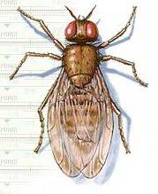
To investigate the impacts of sexual activity on the fruitfly longevity, Partridge and Farquhar (1981), measured the longevity of male fruitflies with access to either one virgin female (potential mate), eight virgin females, one pregnant female (not a potential mate), eight pregnant females or no females. The pool of available male fruitflies varied in size and since size is known to impact longevity, the researchers also measured thorax length as a covariate.

Download Partridge1 data set

Format of partridge1.csv data file

TREATMENT	THORAX	LONGEV
Preg8	0.64	35
Preg8	0.68	37
Preg8	0.68	49
..	..	..

TREATMENT	Categorical listing of the number and sort of female partners(None - no female partners, Preg1 - one pregnant female partner, Preg8 - eight pregnant partners, Virg1 - one virgin female, Virg8 - eight virgin females)
THORAX	Continuous covariate, the length of the thorax (mm)
LONGEV	Longevity of male fruitflies. Response variable.

Open the partridge1 data file. HINT.

Show code

partridge <- read.table("../downloads/data/partridge1.csv", 
    header = T, sep = ",", strip.white = T)
head(partridge)

##   TREATMENT THORAX LONGEV
## 1     Preg8   0.64     35
## 2     Preg8   0.68     37
## 3     Preg8   0.68     49
## 4     Preg8   0.72     46
## 5     Preg8   0.72     63
## 6     Preg8   0.76     39

In the table below, list the assumptions of nested ANOVA along with how violations of each assumption are diagnosed and/or the risks of violations are minimized.

Assumption	Diagnostic/Risk Minimization
I.
II.
III.
IV.
V.

Check the assumptions of normality and homogeneity of variances (HINT). Is there any evidence of violations of the assumptions? (Y or N)
If so, assess whether a transformation will address the violations (HINT).
View full code
plot(aov(LONGEV ~ THORAX + TREATMENT, partridge), which = 1)

Check these assumptions of linearity and homogeneity of slopes EMPIRICALLY (HINT). Is there any evidence of violations of the assumptions? (Y or N)

View full code

anova(aov(log10(LONGEV) ~ THORAX * TREATMENT, partridge))

## Analysis of Variance Table
## 
## Response: log10(LONGEV)
##                   Df Sum Sq Mean Sq F value Pr(>F)    
## THORAX             1  1.212   1.212  176.50 <2e-16 ***
## TREATMENT          4  0.783   0.196   28.50 <2e-16 ***
## THORAX:TREATMENT   4  0.043   0.011    1.56   0.19    
## Residuals        115  0.790   0.007                   
## ---
## Signif. codes:  0 '***' 0.001 '**' 0.01 '*' 0.05 '.' 0.1 ' ' 1

Finally, check that the ranges of the covariate are similar for each level of the categorical variable (HINT). Is there any evidence that the ranges of the covariate differ between the different levels of the categorical variable? (Y or N)

View full code
anova(aov(THORAX ~ TREATMENT, partridge))
## Analysis of Variance Table ## ## Response: THORAX ## Df Sum Sq Mean Sq F value Pr(>F) ## TREATMENT 4 0.030 0.00750 1.26 0.29 ## Residuals 120 0.714 0.00595

Fit the linear model and produce an ANOVA table to test the null hypotheses that there no effects of treatment (female type) on the (log transformed) longevity of male fruitflies adjusted for thorax length. Note that as the design is inherently imbalanced (since there is a different series of thorax lengths within each treatment type), Type I sums of squares are inappropriate. Therefore Type III sums of squares will be used.

In addition to the global Ancova, the researchers likely to have been interested in examining a set of specific planned comparisons. Two such contrasts could be:
1. "pregnant versus virgin partners (to investigate the impacts of any sexual activity)?" (contrast coefficients: 0, .5, .5, -.5, -.5)
2. "one virgin versus eight virgin partners (to investigate the impacts of sexual frequency)?" (contrast coefficients: 0, 0, 0, 1, -1)

Before we fit the linear model (perform the ANOVA), we need to define the contrast coefficients (and thus comparisons) that we wish to perform in addition to the global ANOVA. Define the contrasts for the TREATMENT variable (HINT)

View full code

contrasts(partridge$TREATMENT) <- cbind(c(0, 0.5, 0.5, -0.5, -0.5), c(0, 0, 0, 1, -1))
round(crossprod(contrasts(partridge$TREATMENT)), 1)

##      [,1] [,2] [,3] [,4]
## [1,]    1    0    0    0
## [2,]    0    2    0    0
## [3,]    0    0    1    0
## [4,]    0    0    0    1

If there is no evidence that the assumptions have been violated and the contrasts were successfully defined, run the linear model, check residuals and examine the ANOVA table

View full code

library(biology)
AnovaM(aov(log10(LONGEV) ~ THORAX + TREATMENT, partridge), split = list(TREATMENT = list(`Preg vs Virg` = 1, 
    `1 Virg vs * Virg` = 2)), type = "III")

## Warning: number of items to replace is not a multiple of replacement length

##                                Df Sum Sq Mean Sq F value  Pr(>F)    
## THORAX                          1  1.017   1.017   145.4 < 2e-16 ***
## TREATMENT                       4  0.783   0.196    28.0 2.2e-16 ***
##   TREATMENT: Preg vs Virg       1  0.542   0.542    77.5 1.3e-14 ***
##   TREATMENT: 1 Virg vs * Virg   1  0.199   0.199    28.5 4.6e-07 ***
## Residuals                     119  0.833   0.007                    
## ---
## Signif. codes:  0 '***' 0.001 '**' 0.01 '*' 0.05 '.' 0.1 ' ' 1

View full code for gls

library(nlme)
partridge.lme <- gls(log10(LONGEV) ~ THORAX + TREATMENT, partridge)
anova(partridge.lme, type = "marginal")

## Denom. DF: 119 
##             numDF F-value p-value
## (Intercept)     1   85.73  <.0001
## THORAX          1  145.43  <.0001
## TREATMENT       4   27.97  <.0001

summary(partridge.lme)

## Generalized least squares fit by REML
##   Model: log10(LONGEV) ~ THORAX + TREATMENT 
##   Data: partridge 
##      AIC    BIC logLik
##   -220.8 -201.3  117.4
## 
## Coefficients:
##               Value Std.Error t-value p-value
## (Intercept)  0.7557   0.08162   9.259  0.0000
## THORAX       1.1939   0.09900  12.060  0.0000
## TREATMENT1   0.1473   0.01673   8.802  0.0000
## TREATMENT2   0.0639   0.01197   5.338  0.0000
## TREATMENT3  -0.0259   0.01674  -1.545  0.1250
## TREATMENT4  -0.0314   0.01686  -1.860  0.0654
## 
##  Correlation: 
##            (Intr) THORAX TREATMENT1 TREATMENT2 TREATMENT3
## THORAX     -0.996                                        
## TREATMENT1 -0.019  0.019                                 
## TREATMENT2  0.155 -0.155 -0.003                          
## TREATMENT3  0.032 -0.033 -0.001      0.005               
## TREATMENT4 -0.124  0.125  0.002     -0.019     -0.004    
## 
## Standardized residuals:
##      Min       Q1      Med       Q3      Max 
## -2.71075 -0.69874 -0.04147  0.71687  2.03709 
## 
## Residual standard error: 0.08364 
## Degrees of freedom: 125 total; 119 residual

Present the results of the planned comparisons as part of the following ANOVA table:

Source of Variation	SS	df	MS	F-ratio	Pvalue
THORAX
TREATMENT
Preg vs Virg
1 Virg vs 8 Virg
Residual (within groups)

Heterogeneous slopes

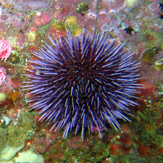
Constable (1993) compared the inter-radial suture widths of urchins maintained on one of three food regimes (Initial: no additional food supplied above what was in the initial sample, low: food supplied periodically and high: food supplied ad libitum. In an attempt to control for substantial variability in urchin sizes, the initial body volume of each urchin was measured as a covariate.

Download Partridge1 data set

Format of constable.csv data file

TREAT	IV	SUTW
Initial	3.5	0.010
Initial	5.0	0.020
Initial	8.0	0.061
..	..	..

TREAT	Categorical listing of the foot treatment (Initial: no additional food supplied above what was in the initial sample, low: food supplied periodically and high: food supplied ad libium)
IV	Continuous covariate, the initial volume of the urchin
SUTW	Width of the suture. Response variable.

Open the constable data file. HINT.

Show code

constable <- read.table("../downloads/data/constable.csv", header = T, sep = ",", strip.white = T)
head(constable)

##     TREAT   IV  SUTW
## 1 Initial  3.5 0.010
## 2 Initial  5.0 0.020
## 3 Initial  8.0 0.061
## 4 Initial 10.0 0.051
## 5 Initial 13.0 0.041
## 6 Initial 13.0 0.061

In the table below, list the assumptions of nested ANOVA along with how violations of each assumption are diagnosed and/or the risks of violations are minimized.

Assumption	Diagnostic/Risk Minimization
I.
II.
III.
IV.
V.

Check the assumptions of normality and homogeneity of variances (HINT). Is there any evidence of violations of the assumptions? (Y or N)
View full code
plot(aov(SUTW ~ I(IV^(1/3)) + TREAT, constable), which = 1)
Check these assumptions of linearity and homogeneity of slopes GRAPHICALLY (HINT). Is there any evidence of violations of the assumptions? (Y or N)
View full code
library(car) scatterplot(SUTW ~ I(IV^(1/3)) | TREAT, constable)

Check these assumptions of linearity and homogeneity of slopes EMPIRICALLY (HINT). Is there any evidence of violations of the assumptions? (Y or N)

View full code

anova(aov(SUTW ~ I(IV^(1/3)) * TREAT, constable))

## Analysis of Variance Table
## 
## Response: SUTW
##                   Df  Sum Sq Mean Sq F value  Pr(>F)    
## I(IV^(1/3))        1 0.00654 0.00654    15.6 0.00019 ***
## TREAT              2 0.01675 0.00838    20.0 1.7e-07 ***
## I(IV^(1/3)):TREAT  2 0.00394 0.00197     4.7 0.01234 *  
## Residuals         66 0.02769 0.00042                    
## ---
## Signif. codes:  0 '***' 0.001 '**' 0.01 '*' 0.05 '.' 0.1 ' ' 1

Finally, check that the ranges of the covariate are similar for each level of the categorical variable (HINT). Is there any evidence that the ranges of the covariate differ between the different levels of the categorical variable? (Y or N)
View full code
anova(aov(I(IV^(1/3)) ~ TREAT, constable))
## Analysis of Variance Table ## ## Response: I(IV^(1/3)) ## Df Sum Sq Mean Sq F value Pr(>F) ## TREAT 2 0.66 0.328 1.36 0.26 ## Residuals 69 16.59 0.240

There is clear evidence that the relationships between suture width and initial volume differ between the three food regimes (slopes are not parallel and a significant interaction between food treatment and initial volume). Regular Ancova is not appropriate.

Determine the regions of difference between each of the food regimes pairwise using the Wilcox modification of the Johnson-Newman procedure (with Games-Howell critical value approximation).

View full code

library(biology)
constable.lm <- lm(SUTW ~ I(IV^(1/3)) * TREAT, constable)
wilcox.JN(constable.lm, type = "H")

##                 df critical value  lower upper
## High vs Initial 37          3.868  3.261 2.187
## High vs Low     34          3.885  6.596 2.264
## Initial vs Low  43          3.839 -1.547 2.939

Present the results of the Wilcox modification of the Johnson-Newman procedure in the following table:>

Comparison df Critical value lower upper
Initial vs low

Initial vs High

Low vs High

How about we finish with a summary graphic?

View full code

# fit the model and Wilcox modification of the Johnson-Newman
library(biology)
constable.lm <- lm(SUTW ~ I(IV^(1/3)) * TREAT, constable)
WJN <- wilcox.JN(constable.lm, type = "H")
# create base plot
plot(SUTW ~ I(IV^(1/3)), constable, type = "n", ylim = c(0, 0.2), xlim = c(3, 50)^(1/3), axes = F, xlab = "", 
    ylab = "")
points(SUTW ~ I(IV^(1/3)), constable[constable$TREAT == "Initial", ], col = "black", pch = 22)
lm1 <- lm(SUTW ~ I(IV^(1/3)), constable, subset = TREAT == "Initial")
abline(lm1, col = "black", lty = 1)
points(SUTW ~ I(IV^(1/3)), constable[constable$TREAT == "Low", ], col = "black", pch = 17)
lm2 <- lm(SUTW ~ I(IV^(1/3)), constable, subset = TREAT == "Low")
abline(lm2, col = "black", lty = 4)
text(SUTW ~ I(IV^(1/3)), "\\#H0844", data = constable[constable$TREAT == "High", ], vfont = c("serif", 
    "plain"))
lm3 <- lm(SUTW ~ I(IV^(1/3)), constable, subset = TREAT == "High")
abline(lm3, col = "black", lty = 2)
axis(1, lab = c(10, 20, 30, 40, 50), at = c(10, 20, 30, 40, 50)^(1/3))
axis(2, las = 1)
mtext("Initial body volume (ml)", 1, line = 3)
mtext("Suture width (mm)", 2, line = 3)
Mpar <- par(family = "HersheySans", font = 2)
library(biology)
# the legend.vfont function facilitates Hershey fonts
legend.vfont("topleft", c("\\#H0841 Initial", "\\#H0844 High", "\\#H0852 Low"), bty = "n", lty = c(1, 
    2, 3), merge = F, title = "Food regime", vfont = c("serif", "plain"))
par(Mpar)
box(bty = "l")
mn <- min(constable$IV^(1/3))
mx <- max(constable$IV^(1/3))
# since lower<upper (lines cross within the range - two regions # of significance (although one is
# outside data range)) region capped to the data range
arrows(WJN[3, 4], 0, mx, 0, ang = 90, length = 0.05, code = 3)
text(mean(c(WJN[3, 4], mx)), 0.003, rownames(WJN)[3])
# since lower>upper (lines cross outside data range region capped to the data range if necessary
arrows(min(WJN[2, 3], mx), 0.01, max(WJN[2, 4], mn), 0.01, ang = 90, length = 0.05, code = 3)
text(mean(c(min(WJN[2, 3], mx), max(WJN[2, 4], mn))), 0.013, rownames(WJN)[2])
# since lower>upper (lines cross outside data range region capped to the data range if necessary
arrows(min(WJN[1, 3], mx), 0.02, max(WJN[1, 4], mn), 0.02, ang = 90, length = 0.05, code = 3)
text(mean(c(min(WJN[1, 3], mx), max(WJN[1, 4], mn))), 0.023, rownames(WJN)[1])