Workshop 9.7b - Mixed effects (multilevel models): Nested designs (Bayesian)
23 April 2011
Nested ANOVA (Mixed effects) references
- McCarthy (2007) - Chpt ?
- Kery (2010) - Chpt ?
- Gelman & Hill (2007) - Chpt ?
- Logan (2010) - Chpt 12
- Quinn & Keough (2002) - Chpt 9
> library(R2jags)
> library(ggplot2)
> library(grid)
> #define my common ggplot options
> murray_opts <- opts(panel.grid.major=theme_blank(),
+ 			   panel.grid.minor=theme_blank(),
+ 			   panel.border = theme_blank(),
+ 			   panel.background = theme_blank(),
+ 			   axis.title.y=theme_text(size=15, vjust=0,angle=90),
+ 			   axis.text.y=theme_text(size=12),
+ 			   axis.title.x=theme_text(size=15, vjust=-1),
+ 			   axis.text.x=theme_text(size=12),
+ 			   axis.line = theme_segment(),
+ 			   legend.position=c(1,0.1),legend.justification=c(1,0),
+ 			   legend.key=theme_blank(),
+ 			   plot.margin=unit(c(0.5,0.5,1,2),"lines")
+ )
>
> #create a convenience function for predicting from mcmc objects
> predict.mcmc <- function(mcmc, terms=NULL, mmat, trans="identity") {
+   library(plyr)
+   library(coda)
+   if(is.null(terms)) mcmc.coefs <- mcmc
+   else 	{
+      iCol<-match(terms, colnames(mcmc))
+ 	 mcmc.coefs <- mcmc[,iCol]
+   }
+   t2=")"
+   if (trans=="identity") {
+ 	t1 <- ""
+ 	t2=""
+   }else if (trans=="log") {
+ 	t1="exp("
+   }else if (trans=="log10") {
+ 	t1="10^("
+   }else if (trans=="sqrt") {
+ 	t1="("
+ 	t2=")^2"
+   }
+   eval(parse(text=paste("mcmc.sum <-adply(mcmc.coefs %*% t(mmat),2,function(x) {
+ 	data.frame(mean=",t1,"mean(x)",t2,",
+     median=",t1,"median(x)",t2,",
+ 	",t1,"coda:::HPDinterval(as.mcmc(x), p=0.68)",t2,",
+ 	",t1,"coda:::HPDinterval(as.mcmc(x))",t2,"
+     )})", sep="")))
+
+   mcmc.sum
+ }
>
>
> #create a convenience function for summarizing mcmc objects
> summary.mcmc <- function(mcmc, terms=NULL, trans="identity") {
+   library(plyr)
+   library(coda)
+   if(is.null(terms)) mcmc.coefs <- mcmc
+   else 	{
+      iCol<-grep(terms, colnames(mcmc))
+ 	 mcmc.coefs <- mcmc[,iCol]
+   }
+   t2=")"
+   if (trans=="identity") {
+ 	t1 <- ""
+ 	t2=""
+   }else if (trans=="log") {
+ 	t1="exp("
+   }else if (trans=="log10") {
+ 	t1="10^("
+   }else if (trans=="sqrt") {
+ 	t1="("
+ 	t2=")^2"
+   }
+   eval(parse(text=paste("mcmc.sum <-adply(mcmc.coefs,2,function(x) {
+ 	data.frame(mean=",t1,"mean(x)",t2,",
+     median=",t1,"median(x)",t2,",
+ 	",t1,"coda:::HPDinterval(as.mcmc(x), p=0.68)",t2,",
+ 	",t1,"coda:::HPDinterval(as.mcmc(x))",t2,"
+     )})", sep="")))
+
+   mcmc.sum$Perc <-100*mcmc.sum$median/sum(mcmc.sum$median)
+   mcmc.sum
+ }
Nested ANOVA
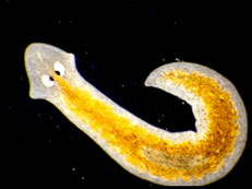
In an unusually detailed preparation for an Environmental Effects Statement for a proposed discharge of dairy wastes into the Curdies River, in western Victoria, a team of stream ecologists wanted to describe the basic patterns of variation in a stream invertebrate thought to be sensitive to nutrient enrichment. As an indicator species, they focused on a small flatworm, Dugesia, and started by sampling populations of this worm at a range of scales. They sampled in two seasons, representing different flow regimes of the river - Winter and Summer. Within each season, they sampled three randomly chosen (well, haphazardly, because sites are nearly always chosen to be close to road access) sites. A total of six sites in all were visited, 3 in each season. At each site, they sampled six stones, and counted the number of flatworms on each stone.
Download Curdies data set| Format of curdies.csv data files | |||||||||||||||||||||||||||||||||||||||||||||
|---|---|---|---|---|---|---|---|---|---|---|---|---|---|---|---|---|---|---|---|---|---|---|---|---|---|---|---|---|---|---|---|---|---|---|---|---|---|---|---|---|---|---|---|---|---|
|
 |
||||||||||||||||||||||||||||||||||||||||||||
> curdies <- read.table("../downloads/data/curdies.csv",
+     header = T, sep = ",", strip.white = T)
> head(curdies)
  SEASON SITE DUGESIA S4DUGES
1 WINTER    1  0.6477  0.8971
2 WINTER    1  6.0962  1.5713
3 WINTER    1  1.3106  1.0700
4 WINTER    1  1.7253  1.1461
5 WINTER    1  1.4594  1.0991
6 WINTER    1  1.0576  1.0141
The hierarchical nature of this design can be appreciated when we examine an illustration of the spatial and temporal scale of the measurements.
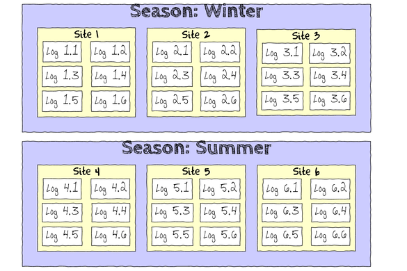
- Within each of the two Seasons, there were three separate Sites (Sites not repeatidly measured across Seasons).
- Within each of the Sites, six logs were selected (haphazardly) from which the number of flatworms were counted.
We construct the model in much the same way. That is:
- The observed number of flatworm per log (for a given Site) is equal to (modelled against) the mean number for that Site
plus a random amount drawn from a normal distribution with a mean of zero and a certain degree of variability (precision).
Number of flatwormlog i = βSite j,i + εi where ε ∼ N(0,σ2)
- The mean number of flatworm per Site (within a given Season) is equal to (modelled against) the mean number for that Season
plus a random amount drawn from a normal distribution with a means of zero and a certain degree of variability (precision).
μSite j = γSeason j + εj where ε ∼ N(0,σ2)
The SITE variable is conveniently already coded as a numeric series (starting at 1).
Exploratory data analysis has indicated that the response variable could be normalized via a forth-root transformation.
- Fit the JAGS model including all pairwise comparisons AND (just because we can), compare the bare surfaces to the surfaces with an algal biofilm. Use with either effects or means parameterization for the 'fixed effects' and means parameterization for the 'random effects'.
Note the following points:
- Non-informative priors for residual precision (standard deviations) should be defined as vague uniform distributions rather than gamma distributions. This prevents the chains from walking to close to parameter estimates of 0.
- Finite-population standard deviation for Site (the within group factor) should reflect standard deviation between Sites within season (not standard deviation between all Sites). Unfortunately, the BUGS language does not offer a mechanism to determine which indexes match certain criteria (for example which Sites correspond to which Season), nor does it allow variables to be redefined. One way to allow us to generate multiple standard deviations is to create an offset vector that can be used to indicate the range of Site numbers that are within which Season.
- As this is a multi-level design in which the Season 'replicates' are determined by the Site means.
It is therefore important that firstly, the number of levels of the within Group factor (Season) reflects
this, and secondly that the
factor levels of the within group factor (Season) correspond to the factor levels of the group factor (Site).
In this case, the Sites are labeled 1-6, but the first three Sites are in Winter. R will naturally label Winter as the second level (as alphabetically W comes after S for summer).
Thus without intervention or careful awareness, it will appear that the Winter means are higher than the Summer means, when it is actually the other way around.
One way to check this, is create the data list and check that all the factor levels are listed in increasing numerical order.
View full code
>
> curdies.list <- with(curdies, list(dugesia = DUGESIA, season = as.numeric(SEASON),
+     site = as.numeric(SITE), n = nrow(curdies), nSeason = length(levels(as.factor(SEASON))),
+     nSite = length(levels(as.factor(SITE))), SiteOffset = c(2, 4, 7)))
> curdies.list
$dugesia
 [1]  0.6477  6.0962  1.3106  1.7253  1.4594  1.0576  1.0163 16.1968  1.1681  1.0243  2.0113  3.6746
[13]  0.6891  1.2191  1.1131  0.6569  0.1361  0.2547  0.0000  0.0000  0.9411  0.0000  0.0000  1.5735
[25]  1.3745  0.0000  0.0000  0.0000  0.0000  0.0000  0.0000  0.0000  0.1329  0.0000  0.6580  0.3745

$season
 [1] 2 2 2 2 2 2 2 2 2 2 2 2 2 2 2 2 2 2 1 1 1 1 1 1 1 1 1 1 1 1 1 1 1 1 1 1

$site
 [1] 1 1 1 1 1 1 2 2 2 2 2 2 3 3 3 3 3 3 4 4 4 4 4 4 5 5 5 5 5 5 6 6 6 6 6 6

$n
[1] 36

$nSeason
[1] 2

$nSite
[1] 6

$SiteOffset
[1] 2 4 7
> ## notice that The Season variable has as many entries as there were plots
> ## rather than having as many as there were Sites.
> ## Also notice that Winter is the second Season according to the factor
> #   levels
>
> season <- with(curdies, SEASON[match(unique(SITE), SITE)])
> season <- factor(season, levels = unique(season))
>
> curdies.list <- with(curdies, list(dugesia = DUGESIA, season = as.numeric(factor(SEASON,
+     levels = c("WINTER", "SUMMER"))), site = as.numeric(SITE), n = nrow(curdies),
+     nSeason = length(levels(as.factor(SEASON))), nSite = length(levels(as.factor(SITE))),
+     SiteOffset = c(2, 4, 7)))
> curdies.list
$dugesia
 [1]  0.6477  6.0962  1.3106  1.7253  1.4594  1.0576  1.0163 16.1968  1.1681  1.0243  2.0113  3.6746
[13]  0.6891  1.2191  1.1131  0.6569  0.1361  0.2547  0.0000  0.0000  0.9411  0.0000  0.0000  1.5735
[25]  1.3745  0.0000  0.0000  0.0000  0.0000  0.0000  0.0000  0.0000  0.1329  0.0000  0.6580  0.3745

$season
 [1] 1 1 1 1 1 1 1 1 1 1 1 1 1 1 1 1 1 1 2 2 2 2 2 2 2 2 2 2 2 2 2 2 2 2 2 2

$site
 [1] 1 1 1 1 1 1 2 2 2 2 2 2 3 3 3 3 3 3 4 4 4 4 4 4 5 5 5 5 5 5 6 6 6 6 6 6

$n
[1] 36

$nSeason
[1] 2

$nSite
[1] 6

$SiteOffset
[1] 2 4 7
> ## That is better
- Effects parameterization
∜dugesiai = βSite j(i) + εi where ε ∼ N(0,σ2)
View full code> > modelString=" + data { + s4dugesia <- sqrt(sqrt(dugesia)) + } + model { + #Likelihood + for (i in 1:n) { + s4dugesia[i]~dnorm(mean[i],tau.res) + mean[i] <- beta.site[site[i]] + y.err[i] <- s4dugesia[i] - mean[1] + } + + #Priors and derivatives + for (j in 1:nSite) { + beta.site[j] ~ dnorm(mean.site[j],tau.site) + mean.site[j] <- gamma0 + gamma.season[season[j]] + } + gamma0 ~ dnorm(0,1.0E-6) + gamma.season[1] <- 0 + for (i in 2:nSeason) { + gamma.season[i] ~ dnorm(0, 1.0E-6) + } + + tau.site <- pow(sigma.site,2) + sigma.site ~ dunif(0,100) + tau.res <- pow(sigma.res,2) + sigma.res ~ dunif(0,100) + + #Season means + Season[1] <- gamma0 + Season[2] <- gamma0+gamma.season[2] + + for (i in 1:nSeason) { + SD.Site[i] <- sd(beta.site[SiteOffset[i]:SiteOffset[i+1]-1]) + } + + + sd.Season <- sd(gamma.season) + sd.Site <- mean(SD.Site) #sd(beta.site) + sd.Resid <- sd(y.err) + } + " > ## write the model to a text file (I suggest you alter the path to somewhere more relevant > ## to your system!) > writeLines(modelString,con="../downloads/BUGSscripts/ws9.7bQ1.1a.txt") > season <- with(curdies,SEASON[match(unique(SITE),SITE)]) > season <- factor(season, levels=unique(season)) > curdies.list <- with(curdies, + list(dugesia=DUGESIA, + season=as.numeric(season),#as.vector(tapply(SEASON,SITE,unique)), + site=as.numeric(SITE), + n=nrow(curdies), nSeason=length(levels(as.factor(SEASON))), + nSite=length(levels(as.factor(SITE))), + SiteOffset=c(2,4,7) + ) + ) > params <- c("beta.site","gamma0","gamma.season","sigma.res","sd.Site","sd.Season","sd.Resid","Season","SD.Site") > adaptSteps = 1000 > burnInSteps = 200 > nChains = 3 > numSavedSteps = 5000 > thinSteps = 10 > nIter = ceiling((numSavedSteps * thinSteps)/nChains) > > library(R2jags) > ## > inits <- list(beta.site=rep(1,6), gamma.season=c(1,1), sigma.res=5, sigma.season=5) > curdies.r2jags <- jags(data=curdies.list, + inits=NULL,#inits=list(inits,inits,inits), # since there are three chains + parameters.to.save=params, + model.file="../downloads/BUGSscripts/ws9.7bQ1.1a.txt", + n.chains=3, + n.iter=nIter, + n.burnin=burnInSteps, + n.thin=thinSteps + )Compiling data graph Resolving undeclared variables Allocating nodes Initializing Reading data back into data table Compiling model graph Resolving undeclared variables Allocating nodes Graph Size: 174 Initializing model
> print(curdies.r2jags)Inference for Bugs model at "../downloads/BUGSscripts/ws9.7bQ1.1a.txt", fit using jags, 3 chains, each with 16667 iterations (first 200 discarded), n.thin = 10 n.sims = 4941 iterations saved mu.vect sd.vect 2.5% 25% 50% 75% 97.5% Rhat n.eff SD.Site[1] 0.020 0.031 0.000 0.005 0.010 0.021 0.107 1.001 3600 SD.Site[2] 0.021 0.024 0.002 0.008 0.013 0.025 0.091 1.001 3700 Season[1] 1.090 0.097 0.903 1.027 1.091 1.152 1.276 1.002 1700 Season[2] 0.293 0.098 0.099 0.230 0.294 0.358 0.477 1.002 1800 beta.site[1] 1.092 0.096 0.902 1.029 1.092 1.154 1.277 1.004 2100 beta.site[2] 1.100 0.099 0.906 1.034 1.098 1.163 1.293 1.003 1200 beta.site[3] 1.077 0.100 0.869 1.013 1.081 1.144 1.261 1.002 1300 beta.site[4] 0.297 0.098 0.099 0.231 0.297 0.361 0.488 1.001 2900 beta.site[5] 0.287 0.098 0.094 0.223 0.288 0.352 0.474 1.002 2300 beta.site[6] 0.298 0.098 0.107 0.234 0.299 0.363 0.489 1.002 1300 gamma.season[1] 0.000 0.000 0.000 0.000 0.000 0.000 0.000 1.000 1 gamma.season[2] -0.797 0.134 -1.055 -0.882 -0.798 -0.712 -0.537 1.004 1500 gamma0 1.090 0.097 0.903 1.027 1.091 1.152 1.276 1.002 1700 sd.Resid 0.547 0.000 0.547 0.547 0.547 0.547 0.547 1.000 1 sd.Season 0.398 0.067 0.269 0.356 0.399 0.441 0.527 1.005 2400 sd.Site 0.021 0.025 0.003 0.008 0.012 0.022 0.092 1.002 2300 sigma.res 2.585 0.311 1.989 2.366 2.591 2.792 3.188 1.001 4900 deviance 35.323 2.670 31.604 33.488 34.753 36.555 42.107 1.003 810 For each parameter, n.eff is a crude measure of effective sample size, and Rhat is the potential scale reduction factor (at convergence, Rhat=1). DIC info (using the rule, pD = var(deviance)/2) pD = 3.6 and DIC = 38.9 DIC is an estimate of expected predictive error (lower deviance is better). - Means parameterization
∜dugesiai = β0 + β1j(i)*phi + β2j(i)*healthi + β3j(i)*phi*healthi + εi where ε ∼ N(0,σ2)View full code> > modelString=" + data { + s4dugesia <- sqrt(sqrt(dugesia)) + } + model { + #Likelihood + for (i in 1:n) { + s4dugesia[i]~dnorm(mean[i],tau.res) + mean[i] <- beta.site[site[i]] + y.err[i] <- s4dugesia[i] - mean[1] + } + + #Priors and derivatives + for (j in 1:nSite) { + beta.site[j] ~ dnorm(mean.site[j],tau.site) + mean.site[j] <- gamma.season[season[j]] + } + for (i in 1:nSeason) { + gamma.season[i] ~ dnorm(0, 1.0E-6) + } + + tau.site <- pow(sigma.site,2) + sigma.site ~ dunif(0,100) + tau.res <- pow(sigma.res,2) + sigma.res ~ dunif(0,100) + + for (i in 1:nSeason) { + SD.Site[i] <- sd(beta.site[SiteOffset[i]:SiteOffset[i+1]-1]) + } + + + sd.Season <- sd(gamma.season) + sd.Site <- mean(SD.Site) #sd(beta.site) + sd.Resid <- sd(y.err) + } + " > ## write the model to a text file (I suggest you alter the path to somewhere more relevant > ## to your system!) > writeLines(modelString,con="../downloads/BUGSscripts/ws9.7bQ1.1b.txt") > > season <- with(curdies,SEASON[match(unique(SITE),SITE)]) > season <- factor(season, levels=unique(season)) > curdies.list <- with(curdies, + list(dugesia=DUGESIA, + season=as.numeric(season),#as.vector(tapply(SEASON,SITE,unique)), + site=as.numeric(SITE), + n=nrow(curdies), nSeason=length(levels(as.factor(SEASON))), + nSite=length(levels(as.factor(SITE))), + SiteOffset=c(2,4,7) + ) + ) > > params <- c("beta.site","gamma.season","sigma.res","sd.Site","sd.Season","sd.Resid") > adaptSteps = 1000 > burnInSteps = 200 > nChains = 3 > numSavedSteps = 5000 > thinSteps = 10 > nIter = ceiling((numSavedSteps * thinSteps)/nChains) > > library(R2jags) > ## > inits <- list(beta.site=rep(1,6), gamma.season=c(1,1), sigma.res=5, sigma.season=5) > curdies.r2jags2 <- jags(data=curdies.list, + inits=NULL,#inits=list(inits,inits,inits), # since there are three chains + parameters.to.save=params, + model.file="../downloads/BUGSscripts/ws9.7bQ1.1b.txt", + n.chains=3, + n.iter=nIter, + n.burnin=burnInSteps, + n.thin=thinSteps + )Compiling data graph Resolving undeclared variables Allocating nodes Initializing Reading data back into data table Compiling model graph Resolving undeclared variables Allocating nodes Graph Size: 171 Initializing model
> print(curdies.r2jags2)Inference for Bugs model at "../downloads/BUGSscripts/ws9.7bQ1.1b.txt", fit using jags, 3 chains, each with 16667 iterations (first 200 discarded), n.thin = 10 n.sims = 4941 iterations saved mu.vect sd.vect 2.5% 25% 50% 75% 97.5% Rhat n.eff beta.site[1] 1.091 0.100 0.896 1.024 1.093 1.158 1.288 1.004 810 beta.site[2] 1.100 0.102 0.907 1.033 1.101 1.168 1.304 1.004 680 beta.site[3] 1.075 0.103 0.863 1.009 1.079 1.145 1.273 1.003 1400 beta.site[4] 0.314 0.095 0.131 0.254 0.313 0.374 0.506 1.001 4900 beta.site[5] 0.303 0.097 0.104 0.243 0.305 0.365 0.493 1.001 4900 beta.site[6] 0.316 0.095 0.130 0.255 0.316 0.376 0.504 1.001 4900 gamma.season[1] 1.088 0.100 0.888 1.022 1.091 1.155 1.284 1.004 1000 gamma.season[2] 0.312 0.093 0.129 0.251 0.311 0.372 0.493 1.001 4900 sd.Resid 0.547 0.000 0.547 0.547 0.547 0.547 0.547 1.000 1 sd.Season 0.388 0.069 0.247 0.344 0.389 0.433 0.521 1.002 1600 sd.Site 0.022 0.026 0.003 0.008 0.013 0.024 0.103 1.002 3200 sigma.res 2.595 0.317 1.993 2.375 2.593 2.807 3.225 1.001 4900 deviance 35.309 2.685 31.524 33.491 34.742 36.574 42.091 1.001 4900 For each parameter, n.eff is a crude measure of effective sample size, and Rhat is the potential scale reduction factor (at convergence, Rhat=1). DIC info (using the rule, pD = var(deviance)/2) pD = 3.6 and DIC = 38.9 DIC is an estimate of expected predictive error (lower deviance is better).
- Before fully exploring the parameters, it is prudent to examine the convergence and mixing diagnostics.
Chose either the effects or means parameterization model (they should yield much the same).
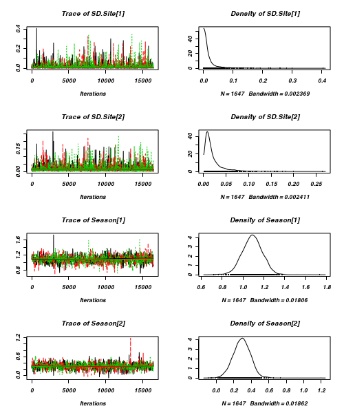
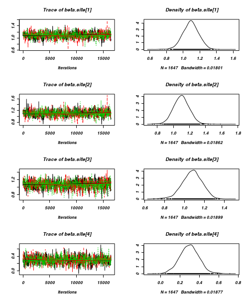
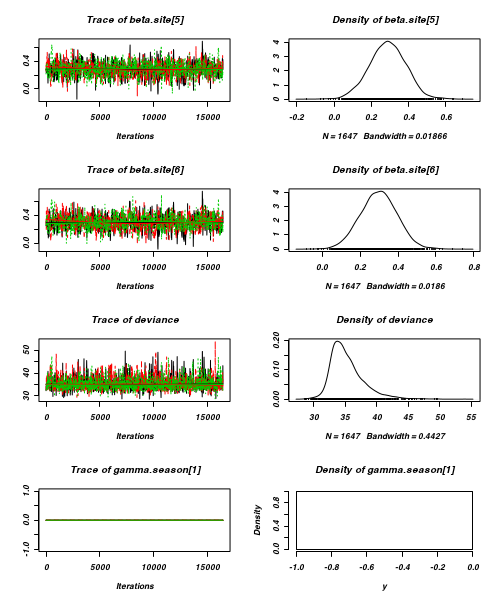
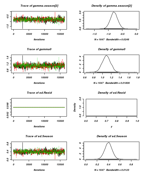
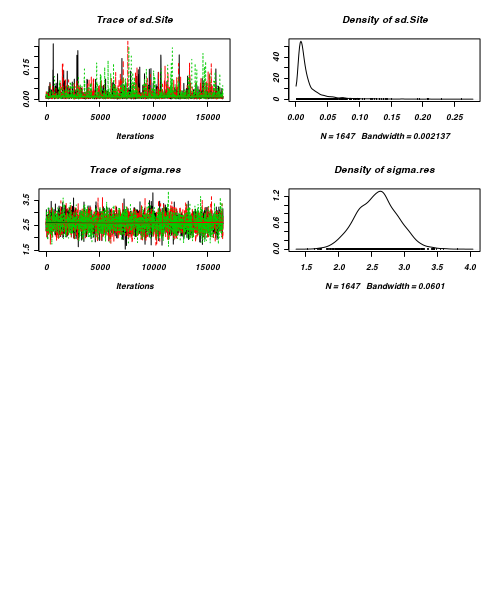
- Trace plots
View code
> plot(as.mcmc(curdies.r2jags))
- Raftery diagnostic
View code
> raftery.diag(as.mcmc(curdies.r2jags))
[[1]] Quantile (q) = 0.025 Accuracy (r) = +/- 0.005 Probability (s) = 0.95 You need a sample size of at least 3746 with these values of q, r and s [[2]] Quantile (q) = 0.025 Accuracy (r) = +/- 0.005 Probability (s) = 0.95 You need a sample size of at least 3746 with these values of q, r and s [[3]] Quantile (q) = 0.025 Accuracy (r) = +/- 0.005 Probability (s) = 0.95 You need a sample size of at least 3746 with these values of q, r and s
- Autocorrelation
View code
> autocorr.diag(as.mcmc(curdies.r2jags))
SD.Site[1] SD.Site[2] Season[1] Season[2] beta.site[1] beta.site[2] beta.site[3] Lag 0 1.0000000 1.000000 1.000000 1.000000 1.000000 1.000000 1.000000 Lag 10 0.2435162 0.292914 0.646960 0.661778 0.637729 0.622426 0.626530 Lag 50 0.0004563 0.010823 0.218858 0.225746 0.220377 0.211287 0.205929 Lag 100 -0.0027200 0.012635 0.090499 0.023267 0.106733 0.074554 0.093988 Lag 500 -0.0194188 -0.007059 -0.004256 -0.008549 -0.002724 -0.004583 -0.007775 beta.site[4] beta.site[5] beta.site[6] deviance gamma.season[1] gamma.season[2] gamma0 Lag 0 1.000000 1.000000 1.00000 1.000000 NaN 1.000000 1.000000 Lag 10 0.647766 0.621643 0.65337 0.372177 NaN 0.630692 0.646960 Lag 50 0.228936 0.198313 0.21387 0.091986 NaN 0.191301 0.218858 Lag 100 0.037973 0.001276 0.03816 0.004202 NaN 0.037074 0.090499 Lag 500 -0.008321 0.005611 -0.01074 -0.010590 NaN -0.002078 -0.004256 sd.Resid sd.Season sd.Site sigma.res Lag 0 1.0000 1.000000 1.000000 1.000000 Lag 10 0.1769 0.630692 0.334801 0.050602 Lag 50 0.1765 0.191301 0.010213 0.014573 Lag 100 0.1620 0.037074 0.007123 0.002961 Lag 500 0.1631 -0.002078 -0.023623 -0.020900
- Trace plots
-
It would seem prudent to re-fit with a thinning factor of 100
View full code
> params <- c("beta.site","gamma0","gamma.season","sigma.res","sd.Site","sd.Season","sd.Resid","Season") > > adaptSteps = 1000 > burnInSteps = 200 > nChains = 3 > numSavedSteps = 5000 > thinSteps = 100 > nIter = ceiling((numSavedSteps * thinSteps)/nChains) > > library(R2jags) > ## > inits <- list(beta.site=rep(1,6), gamma.season=c(1,1), sigma.res=5, sigma.season=5) > curdies.r2jags3 <- jags(data=curdies.list, + inits=NULL,#inits=list(inits,inits,inits), # since there are three chains + parameters.to.save=params, + model.file="../downloads/BUGSscripts/ws9.7bQ1.1a.txt", + n.chains=3, + n.iter=nIter, + n.burnin=burnInSteps, + n.thin=thinSteps + )
Compiling data graph
   Resolving undeclared variables
   Allocating nodes
   Initializing
   Reading data back into data table
Compiling model graph
   Resolving undeclared variables
   Allocating nodes
   Graph Size: 174

Initializing model
> print(curdies.r2jags3)Inference for Bugs model at "../downloads/BUGSscripts/ws9.7bQ1.1a.txt", fit using jags, 3 chains, each with 166667 iterations (first 200 discarded), n.thin = 100 n.sims = 4995 iterations saved mu.vect sd.vect 2.5% 25% 50% 75% 97.5% Rhat n.eff Season[1] 1.088 0.100 0.895 1.023 1.087 1.153 1.285 1.001 5000 Season[2] 0.303 0.097 0.109 0.240 0.305 0.367 0.495 1.001 3800 beta.site[1] 1.091 0.101 0.897 1.025 1.089 1.156 1.292 1.002 2200 beta.site[2] 1.098 0.103 0.897 1.030 1.097 1.164 1.305 1.001 5000 beta.site[3] 1.075 0.103 0.865 1.009 1.076 1.142 1.274 1.002 2100 beta.site[4] 0.306 0.099 0.109 0.240 0.306 0.370 0.499 1.001 5000 beta.site[5] 0.295 0.099 0.094 0.229 0.297 0.362 0.485 1.002 2300 beta.site[6] 0.309 0.099 0.112 0.243 0.309 0.375 0.504 1.001 5000 gamma.season[1] 0.000 0.000 0.000 0.000 0.000 0.000 0.000 1.000 1 gamma.season[2] -0.785 0.141 -1.062 -0.879 -0.785 -0.694 -0.510 1.001 3900 gamma0 1.088 0.100 0.895 1.023 1.087 1.153 1.285 1.001 5000 sd.Resid 0.547 0.000 0.547 0.547 0.547 0.547 0.547 1.000 1 sd.Season 0.392 0.070 0.255 0.347 0.392 0.439 0.531 1.001 3300 sd.Site 0.021 0.026 0.003 0.007 0.012 0.023 0.100 1.001 3900 sigma.res 2.579 0.307 1.995 2.365 2.575 2.783 3.192 1.001 5000 deviance 35.365 2.662 31.586 33.546 34.826 36.632 42.115 1.002 1900 For each parameter, n.eff is a crude measure of effective sample size, and Rhat is the potential scale reduction factor (at convergence, Rhat=1). DIC info (using the rule, pD = var(deviance)/2) pD = 3.5 and DIC = 38.9 DIC is an estimate of expected predictive error (lower deviance is better). -
A summary figure would be nice
View code
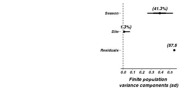
> curdies.mcmc <- as.mcmc(curdies.r2jags3$BUGSoutput$sims.matrix)
> #get the column indexes for the parameters we are interested in
> curdies.sum <- summary.mcmc(curdies.mcmc, terms=c("^Season")) #or "alpha"
> curdies.sum$Season <- c("Winter","Summer")
>
> p1<-ggplot(curdies.sum,aes(y=mean, x=Season))+
+ geom_errorbar(aes(ymin=lower, ymax=upper),width=0,size=1.5,position=position_dodge(0.2))+
+ geom_errorbar(aes(ymin=lower.1, ymax=upper.1),width=0,position=position_dodge(0.2))+
+ geom_point(size=3)+
+ scale_y_continuous("Number of flatworms",
+    trans=trans_new("x4",function(x) x^4, function(x) sqrt(sqrt(x))),
+    breaks=sqrt(sqrt(pretty(c(0,3)))),
+    labels=pretty(c(0,3)))+
+ scale_x_discrete("Season")+
+ murray_opts
>
> #Finite-population standard deviations
> curdies.sd <- summary.mcmc(curdies.mcmc, terms=c("sd"))
> rownames(curdies.sd) <- c("Residuals", "Season", "Site")
> curdies.sd$name <- factor(c("Residuals", "Season", "Site"), levels=c("Residuals", "Site", "Season"))
>
> p2<-ggplot(curdies.sd,aes(y=name, x=median))+
+ geom_vline(xintercept=0,linetype="dashed")+
+ geom_hline(xintercept=0)+
+ scale_x_continuous("Finite population \nvariance components (sd)")+
+ geom_errorbarh(aes(xmin=lower.1, xmax=upper.1), height=0, size=1)+
+ geom_errorbarh(aes(xmin=lower, xmax=upper), height=0, size=1.5)+
+ geom_point(size=3)+
+ geom_text(aes(label=sprintf("(%4.1f%%)",Perc),vjust=-1))+
+ murray_opts+
+ opts(axis.line=theme_blank(),axis.title.y=theme_blank(),
+ axis.text.y=theme_text(size=12,hjust=1))
>
> grid.newpage()
> pushViewport(viewport(layout=grid.layout(1,2,5,5,respect=TRUE)))
> pushViewport(viewport(layout.pos.col=1, layout.pos.row=1))
> print(p1,newpage=FALSE)
Error: Breaks and labels are different lengths
> popViewport(1)
> pushViewport(viewport(layout.pos.col=2, layout.pos.row=1))
> print(p2,newpage=FALSE)
> popViewport(0)