Workshop 9.6b - Factorial ANOVA (Bayesian)
23 April 2011
Factorial ANOVA references
- McCarthy (2007) - Chpt 6
- Kery (2010) - Chpt 10
- Gelman & Hill (2007) - Chpt 4
- Logan (2010) - Chpt 12
- Quinn & Keough (2002) - Chpt 9
> library(R2jags)
> library(ggplot2)
> library(grid)
> #define my common ggplot options
> murray_opts <- opts(panel.grid.major=theme_blank(),
+                            panel.grid.minor=theme_blank(),
+                            panel.border = theme_blank(),
+                            panel.background = theme_blank(),
+                            axis.title.y=theme_text(size=15, vjust=0,angle=90),
+                            axis.text.y=theme_text(size=12),
+                            axis.title.x=theme_text(size=15, vjust=-1),
+                            axis.text.x=theme_text(size=12),
+                            axis.line = theme_segment(),
+                            legend.position=c(1,0.1),legend.justification=c(1,0),
+                            legend.key=theme_blank(),
+                            plot.margin=unit(c(0.5,0.5,1,2),"lines")
+ )
>
> #create a convenience function for predicting from mcmc objects
> predict.mcmc <- function(mcmc, terms=NULL, mmat, trans="identity") {
+   library(plyr)
+   library(coda)
+   if(is.null(terms)) mcmc.coefs <- mcmc
+   else  {
+      iCol<-match(terms, colnames(mcmc))
+          mcmc.coefs <- mcmc[,iCol]
+   }
+   t2=")"
+   if (trans=="identity") {
+         t1 <- ""
+         t2=""
+   }else if (trans=="log") {
+         t1="exp("
+   }else if (trans=="log10") {
+         t1="10^("
+   }else if (trans=="sqrt") {
+         t1="("
+         t2=")^2"
+   }
+   eval(parse(text=paste("mcmc.sum <-adply(mcmc.coefs %*% t(mmat),2,function(x) {
	data.frame(mean=",t1,"mean(x)",t2,",
    median=",t1,"median(x)",t2,",
	",t1,"coda:::HPDinterval(as.mcmc(x), p=0.68)",t2,",
	",t1,"coda:::HPDinterval(as.mcmc(x))",t2,"
    )})", sep="")))
+
+   mcmc.sum
+ }
>
>
> #create a convenience function for summarizing mcmc objects
> summary.mcmc <- function(mcmc, terms=NULL, trans="identity") {
+   library(plyr)
+   library(coda)
+   if(is.null(terms)) mcmc.coefs <- mcmc
+   else  {
+      iCol<-grep(terms, colnames(mcmc))
+          mcmc.coefs <- mcmc[,iCol]
+   }
+   t2=")"
+   if (trans=="identity") {
+         t1 <- ""
+         t2=""
+   }else if (trans=="log") {
+         t1="exp("
+   }else if (trans=="log10") {
+         t1="10^("
+   }else if (trans=="sqrt") {
+         t1="("
+         t2=")^2"
+   }
+   eval(parse(text=paste("mcmc.sum <-adply(mcmc.coefs,2,function(x) {
	data.frame(mean=",t1,"mean(x)",t2,",
    median=",t1,"median(x)",t2,",
	",t1,"coda:::HPDinterval(as.mcmc(x), p=0.68)",t2,",
	",t1,"coda:::HPDinterval(as.mcmc(x))",t2,"
    )})", sep="")))
+
+   mcmc.sum$Perc <-100*mcmc.sum$median/sum(mcmc.sum$median)
+   mcmc.sum
+ }
Two-factor ANOVA
A biologist studying starlings wanted to know whether the mean mass of starlings differed according to different roosting situations. She was also interested in whether the mean mass of starlings altered over winter (Northern hemisphere) and whether the patterns amongst roosting situations were consistent throughout winter, therefore starlings were captured at the start (November) and end of winter (January). Ten starlings were captured from each roosting situation in each season, so in total, 80 birds were captured and weighed.
Download Starling data set| Format of starling.csv data files | |||||||||||||||||||||||||||||||||||||||||||||||||||||
|---|---|---|---|---|---|---|---|---|---|---|---|---|---|---|---|---|---|---|---|---|---|---|---|---|---|---|---|---|---|---|---|---|---|---|---|---|---|---|---|---|---|---|---|---|---|---|---|---|---|---|---|---|---|
|
 |
||||||||||||||||||||||||||||||||||||||||||||||||||||
Open the starling data file.
> starling <- read.table("../downloads/data/starling.csv",
+     header = T, sep = ",", strip.white = T)
> head(starling)
  SITUATION    MONTH MASS GROUP
1        S1 November   78 S1Nov
2        S1 November   88 S1Nov
3        S1 November   87 S1Nov
4        S1 November   88 S1Nov
5        S1 November   83 S1Nov
6        S1 November   82 S1Nov
Exploratory data analysis did not reveal any issues with normality or homogeneity of variance.
- Fit the JAGS model including all pairwise comparisons AND (just because we can), compare the bare surfaces to the surfaces with an algal biofilm. Use with either:
- Effects parameterization
massi = β0 + β1j(i)*monthi + β2j(i)*situationi + β3j(i)*monthi*situationi + εi where ε ∼ N(0,σ2)View full code> modelString=" model { #Likelihood for (i in 1:n) { mass[i]~dnorm(mean[i],tau.res) mean[i] <- beta0+beta.month[month[i]]+beta.situation[situation[i]]+ beta.int[month[i],situation[i]] y.err[i] <- mass[i] - mean[i] } #Priors and derivatives beta0 ~ dnorm(0,1.0E-6) beta.month[1] <- 0 beta.int[1,1] <- 0 for (i in 2:nMonth) { beta.month[i] ~ dnorm(0.001, 1.0E-6) #prior beta.int[i,1] <- 0 } beta.situation[1] <- 0 for (i in 2:nSituation){ beta.situation[i] ~ dnorm(0.001, 1.0E-6) #prior cannot be 0, or else will have an ##init of zero and then will be dividing by zero when calculating cohen's D beta.int[1,i] <- 0 } for (i in 2:nMonth) { for (j in 2:nSituation){ beta.int[i,j] ~ dnorm(0, 1.0E-6) } } #Means for (i in 1:nMonth) { for (j in 1:nSituation) { Mean[i,j] <- beta0 + beta.month[i] + beta.situation[j] + beta.int[i,j] } } sigma.res ~ dgamma(0.001, 0.001) #prior on sd residuals tau.res <- 1 / (sigma.res * sigma.res) sd.Month <- sd(beta.month[]) sd.Situation <- sd(beta.situation[]) sd.Int <- sd(beta.int[,]) sd.Resid <- sd(y.err[]) #Pairwise comparisons of situations for (i in 1:nSituation) { for (j in 1:nSituation) { eff[i,j] <- (beta.situation[i] - beta.situation[j]) } } #Effects of month within each situation for (i in 1:nSituation) { eff2[i] <- Mean[1,i] - Mean[2,i] } } " > ## write the model to a text file (I suggest you alter the path to somewhere more relevant > ## to your system!) > writeLines(modelString,con="../downloads/BUGSscripts/ws9.6bQ1.1a.txt") > starling.list <- with(starling, + list(mass=MASS, + month=as.numeric(MONTH), situation=as.numeric(SITUATION), + n=nrow(starling), nMonth=length(levels(MONTH)), + nSituation=length(levels(SITUATION)) + ) + ) > > params <- c("beta0","beta.month","beta.situation","beta.int","sigma.res","sd.Month","sd.Situation","sd.Int","sd.Resid", "Mean","eff","eff2") > adaptSteps = 1000 > burnInSteps = 200 > nChains = 3 > numSavedSteps = 5000 > thinSteps = 10 > nIter = ceiling((numSavedSteps * thinSteps)/nChains) > > library(R2jags) > ## > starling.r2jags <- jags(data=starling.list, + inits=NULL, #or inits=list(inits,inits,inits) # since there are three chains + parameters.to.save=params, + model.file="../downloads/BUGSscripts/ws9.6bQ1.1a.txt", + n.chains=3, + n.iter=nIter, + n.burnin=burnInSteps, + n.thin=thinSteps + )
Compiling model graph
   Resolving undeclared variables
   Allocating nodes
   Graph Size: 367

Initializing model
> print(starling.r2jags)
Inference for Bugs model at "../downloads/BUGSscripts/ws9.6bQ1.1a.txt", fit using jags, 3 chains, each with 16667 iterations (first 200 discarded), n.thin = 10 n.sims = 4941 iterations saved mu.vect sd.vect 2.5% 25% 50% 75% 97.5% Rhat n.eff Mean[1,1] 90.770 1.368 88.088 89.864 90.750 91.695 93.470 1.001 4900 Mean[2,1] 83.630 1.342 80.970 82.743 83.623 84.520 86.276 1.001 4900 Mean[1,2] 90.159 1.348 87.482 89.264 90.161 91.045 92.819 1.001 4900 Mean[2,2] 79.401 1.348 76.754 78.510 79.401 80.284 82.053 1.001 4900 Mean[1,3] 88.211 1.348 85.561 87.329 88.206 89.106 90.850 1.001 4200 Mean[2,3] 78.593 1.341 75.931 77.692 78.588 79.492 81.244 1.001 4900 Mean[1,4] 84.206 1.354 81.575 83.272 84.202 85.124 86.843 1.002 2300 Mean[2,4] 75.438 1.353 72.744 74.560 75.443 76.336 78.079 1.001 4900 beta.int[1,1] 0.000 0.000 0.000 0.000 0.000 0.000 0.000 1.000 1 beta.int[2,1] 0.000 0.000 0.000 0.000 0.000 0.000 0.000 1.000 1 beta.int[1,2] 0.000 0.000 0.000 0.000 0.000 0.000 0.000 1.000 1 beta.int[2,2] -3.618 2.741 -9.114 -5.424 -3.608 -1.854 1.970 1.001 4900 beta.int[1,3] 0.000 0.000 0.000 0.000 0.000 0.000 0.000 1.000 1 beta.int[2,3] -2.478 2.745 -7.906 -4.302 -2.465 -0.639 2.888 1.001 4800 beta.int[1,4] 0.000 0.000 0.000 0.000 0.000 0.000 0.000 1.000 1 beta.int[2,4] -1.628 2.720 -6.953 -3.497 -1.603 0.259 3.625 1.001 4900 beta.month[1] 0.000 0.000 0.000 0.000 0.000 0.000 0.000 1.000 1 beta.month[2] -7.140 1.943 -10.964 -8.441 -7.137 -5.837 -3.421 1.001 4900 beta.situation[1] 0.000 0.000 0.000 0.000 0.000 0.000 0.000 1.000 1 beta.situation[2] -0.611 1.917 -4.434 -1.894 -0.582 0.672 3.168 1.001 4900 beta.situation[3] -2.559 1.900 -6.357 -3.805 -2.557 -1.335 1.222 1.001 2800 beta.situation[4] -6.564 1.938 -10.448 -7.838 -6.562 -5.261 -2.807 1.001 4900 beta0 90.770 1.368 88.088 89.864 90.750 91.695 93.470 1.001 4900 eff[1,1] 0.000 0.000 0.000 0.000 0.000 0.000 0.000 1.000 1 eff[2,1] -0.611 1.917 -4.434 -1.894 -0.582 0.672 3.168 1.001 4900 eff[3,1] -2.559 1.900 -6.357 -3.805 -2.557 -1.335 1.222 1.001 2800 eff[4,1] -6.564 1.938 -10.448 -7.838 -6.562 -5.261 -2.807 1.001 4900 eff[1,2] 0.611 1.917 -3.168 -0.672 0.582 1.894 4.434 1.001 4900 eff[2,2] 0.000 0.000 0.000 0.000 0.000 0.000 0.000 1.000 1 eff[3,2] -1.948 1.906 -5.640 -3.226 -1.960 -0.673 1.807 1.001 3200 eff[4,2] -5.953 1.897 -9.722 -7.190 -5.958 -4.696 -2.243 1.001 3800 eff[1,3] 2.559 1.900 -1.222 1.335 2.557 3.805 6.357 1.001 2800 eff[2,3] 1.948 1.906 -1.807 0.673 1.960 3.226 5.640 1.001 3200 eff[3,3] 0.000 0.000 0.000 0.000 0.000 0.000 0.000 1.000 1 eff[4,3] -4.005 1.896 -7.681 -5.283 -3.979 -2.766 -0.270 1.002 2000 eff[1,4] 6.564 1.938 2.807 5.261 6.562 7.838 10.448 1.001 4900 eff[2,4] 5.953 1.897 2.243 4.696 5.958 7.190 9.722 1.001 3800 eff[3,4] 4.005 1.896 0.270 2.766 3.979 5.283 7.681 1.002 2000 eff[4,4] 0.000 0.000 0.000 0.000 0.000 0.000 0.000 1.000 1 eff2[1] 7.140 1.943 3.421 5.837 7.137 8.441 10.964 1.004 4900 eff2[2] 10.758 1.931 6.988 9.493 10.754 12.027 14.569 1.001 4900 eff2[3] 9.618 1.918 5.815 8.290 9.647 10.909 13.365 1.001 4900 eff2[4] 8.768 1.878 5.189 7.496 8.742 9.981 12.466 1.002 4900 sd.Int 1.803 0.803 0.516 1.206 1.702 2.306 3.631 1.001 4900 sd.Month 3.570 0.972 1.710 2.918 3.568 4.221 5.482 1.004 4900 sd.Resid 4.185 0.108 4.035 4.106 4.166 4.242 4.446 1.002 1700 sd.Situation 2.741 0.657 1.475 2.296 2.735 3.175 4.089 1.001 3300 sigma.res 4.257 0.358 3.649 4.003 4.235 4.475 5.033 1.001 4900 deviance 457.997 4.558 451.319 454.640 457.201 460.513 468.982 1.002 1700 For each parameter, n.eff is a crude measure of effective sample size, and Rhat is the potential scale reduction factor (at convergence, Rhat=1). DIC info (using the rule, pD = var(deviance)/2) pD = 10.4 and DIC = 468.4 DIC is an estimate of expected predictive error (lower deviance is better). - Means parameterization
massi = αj(i)*monthi*situationi + εi where ε ∼ N(0,σ2)View full code
> modelString="
model {
   #Likelihood
   for (i in 1:n) {
      mass[i]~dnorm(mean[i],tau.res)
      mean[i] <- alpha[month[i],situation[i]]
      y.err[i] <- mass[i] - mean[i]
   }

   #Priors and derivatives
   for (i in 1:nMonth) {
     for (j in 1:nSituation){
       alpha[i,j] ~ dnorm(0, 1.0E-6)
     }
   }

   sigma.res ~ dgamma(0.001, 0.001) #prior on sd residuals
   tau.res <- 1 / (sigma.res * sigma.res)

   #Effects
   beta0 <- alpha[1,1]
   for (i in 1:nMonth) {
     beta.month[i] <- alpha[i,1]-beta0
   }
   for (i in 1:nSituation) {
     beta.situation[i] <- alpha[1,i]-beta0
   }

   for (i in 1:nMonth) {
     for (j in 1:nSituation) {
	   beta.int[i,j] <- alpha[i,j]-beta.month[i]-beta.situation[j]-beta0
	 }
   }
   sd.Month <- sd(beta.month[])
   sd.Situation <- sd(beta.situation[])
   sd.Int <- sd(beta.int[,])
   sd.Resid <- sd(y.err[])

   #Pairwise comparisons of situations
   for (i in 1:nSituation) {
     for (j in 1:nSituation) {
	   eff[i,j] <- beta.situation[i] - beta.situation[j]
	 }
   }
   #Effects of month within each situation
   for (i in 1:nSituation) {
      eff2[i] <- alpha[1,i] - alpha[2,i]
   }
 }
"
> ## write the model to a text file (I suggest you alter the path to somewhere more relevant
> ## to your system!)
> writeLines(modelString,con="../downloads/BUGSscripts/ws9.6bQ1.1b.txt")
> starling.list <- with(starling,
+                          list(mass=MASS,
+                          month=as.numeric(MONTH), situation=as.numeric(SITUATION),
+                                  n=nrow(starling), nMonth=length(levels(MONTH)),
+                                  nSituation=length(levels(SITUATION))
+                         )
+            )
>
> params <- c("beta.month","beta.situation","beta.int","sigma.res","sd.Month","sd.Situation","sd.Int","sd.Resid", "eff","eff2")
> adaptSteps = 1000
> burnInSteps = 200
> nChains = 3
> numSavedSteps = 5000
> thinSteps = 10
> nIter = ceiling((numSavedSteps * thinSteps)/nChains)
>
> library(R2jags)
> ##
> starling.r2jags2 <- jags(data=starling.list,
+           inits=NULL, #or inits=list(inits,inits,inits) # since there are three chains
+           parameters.to.save=params,
+           model.file="../downloads/BUGSscripts/ws9.6bQ1.1b.txt",
+           n.chains=3,
+           n.iter=nIter,
+           n.burnin=burnInSteps,
+       n.thin=thinSteps
+           )
Compiling model graph
   Resolving undeclared variables
   Allocating nodes
   Graph Size: 381

Initializing model
> print(starling.r2jags2)
Inference for Bugs model at "../downloads/BUGSscripts/ws9.6bQ1.1b.txt", fit using jags, 3 chains, each with 16667 iterations (first 200 discarded), n.thin = 10 n.sims = 4941 iterations saved mu.vect sd.vect 2.5% 25% 50% 75% 97.5% Rhat n.eff beta.int[1,1] 0.000 0.000 0.000 0.000 0.000 0.000 0.000 1.000 1 beta.int[2,1] 0.000 0.000 0.000 0.000 0.000 0.000 0.000 1.000 1 beta.int[1,2] 0.000 0.000 0.000 0.000 0.000 0.000 0.000 1.000 1 beta.int[2,2] -3.566 2.721 -8.826 -5.398 -3.568 -1.710 1.735 1.001 4900 beta.int[1,3] 0.000 0.000 0.000 0.000 0.000 0.000 0.000 1.000 1 beta.int[2,3] -2.402 2.666 -7.569 -4.189 -2.387 -0.634 2.796 1.002 1100 beta.int[1,4] 0.000 0.000 0.000 0.000 0.000 0.000 0.000 1.000 1 beta.int[2,4] -1.568 2.725 -6.805 -3.450 -1.564 0.321 3.712 1.002 1500 beta.month[1] 0.000 0.000 0.000 0.000 0.000 0.000 0.000 1.000 1 beta.month[2] -7.203 1.919 -10.918 -8.490 -7.208 -5.906 -3.403 1.002 2200 beta.situation[1] 0.000 0.000 0.000 0.000 0.000 0.000 0.000 1.000 1 beta.situation[2] -0.648 1.921 -4.359 -1.946 -0.637 0.616 3.119 1.001 4900 beta.situation[3] -2.604 1.892 -6.204 -3.883 -2.642 -1.322 1.198 1.001 4900 beta.situation[4] -6.639 1.913 -10.306 -7.943 -6.645 -5.333 -2.831 1.002 2300 eff[1,1] 0.000 0.000 0.000 0.000 0.000 0.000 0.000 1.000 1 eff[2,1] -0.648 1.921 -4.359 -1.946 -0.637 0.616 3.119 1.001 4900 eff[3,1] -2.604 1.892 -6.204 -3.883 -2.642 -1.322 1.198 1.001 4900 eff[4,1] -6.639 1.913 -10.306 -7.943 -6.645 -5.333 -2.831 1.002 2300 eff[1,2] 0.648 1.921 -3.119 -0.616 0.637 1.946 4.359 1.001 4900 eff[2,2] 0.000 0.000 0.000 0.000 0.000 0.000 0.000 1.000 1 eff[3,2] -1.956 1.914 -5.707 -3.223 -1.957 -0.648 1.726 1.001 4900 eff[4,2] -5.991 1.894 -9.677 -7.263 -5.999 -4.747 -2.186 1.002 1800 eff[1,3] 2.604 1.892 -1.198 1.322 2.642 3.883 6.204 1.001 4900 eff[2,3] 1.956 1.914 -1.726 0.648 1.957 3.223 5.707 1.001 4900 eff[3,3] 0.000 0.000 0.000 0.000 0.000 0.000 0.000 1.000 1 eff[4,3] -4.035 1.904 -7.732 -5.325 -4.031 -2.746 -0.327 1.001 3900 eff[1,4] 6.639 1.913 2.831 5.333 6.645 7.943 10.306 1.002 2300 eff[2,4] 5.991 1.894 2.186 4.747 5.999 7.263 9.677 1.002 1800 eff[3,4] 4.035 1.904 0.327 2.746 4.031 5.325 7.732 1.001 3900 eff[4,4] 0.000 0.000 0.000 0.000 0.000 0.000 0.000 1.000 1 eff2[1] 7.203 1.919 3.403 5.906 7.208 8.490 10.918 1.001 3300 eff2[2] 10.769 1.898 7.117 9.512 10.798 12.029 14.455 1.001 4900 eff2[3] 9.605 1.904 5.859 8.338 9.627 10.853 13.318 1.004 1200 eff2[4] 8.772 1.916 5.019 7.474 8.779 10.084 12.475 1.001 4400 sd.Int 1.779 0.787 0.508 1.195 1.698 2.287 3.499 1.001 4900 sd.Month 3.602 0.960 1.701 2.953 3.604 4.245 5.459 1.001 3300 sd.Resid 4.184 0.104 4.037 4.108 4.167 4.237 4.431 1.001 4900 sd.Situation 2.766 0.644 1.503 2.339 2.768 3.199 4.013 1.002 1800 sigma.res 4.253 0.358 3.626 4.001 4.229 4.476 5.011 1.002 1400 deviance 458.035 4.463 451.313 454.807 457.362 460.524 468.601 1.001 4900 For each parameter, n.eff is a crude measure of effective sample size, and Rhat is the potential scale reduction factor (at convergence, Rhat=1). DIC info (using the rule, pD = var(deviance)/2) pD = 10.0 and DIC = 468.0 DIC is an estimate of expected predictive error (lower deviance is better). - Before fully exploring the parameters, it is prudent to examine the convergence and mixing diagnostics.
Chose either the effects or means parameterization model (they should yield much the same).
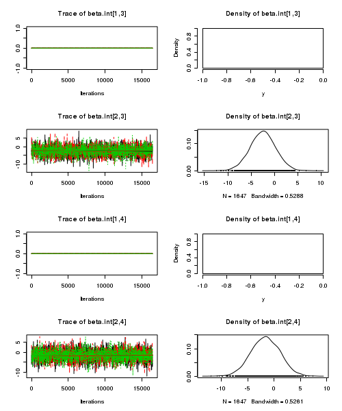
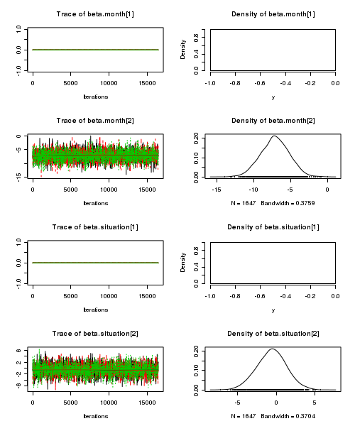
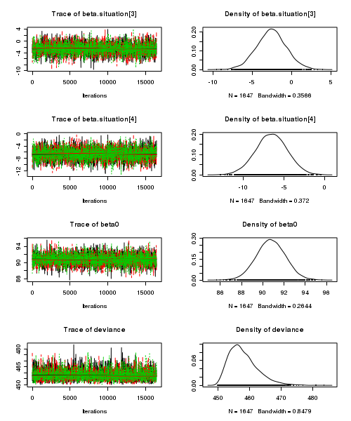
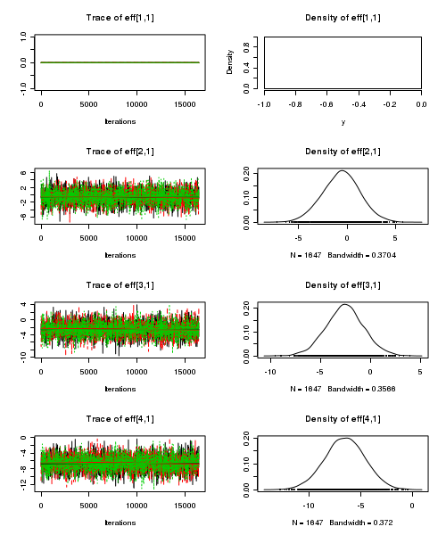
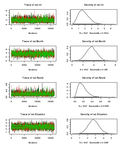
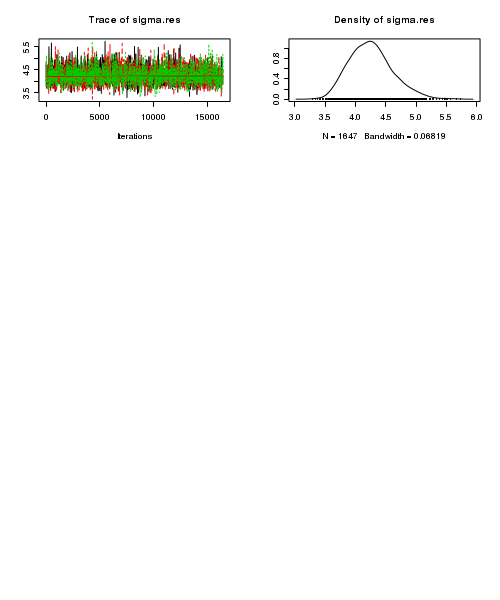
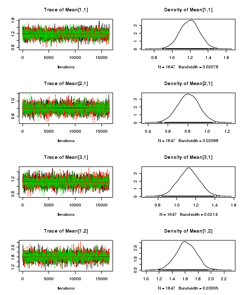
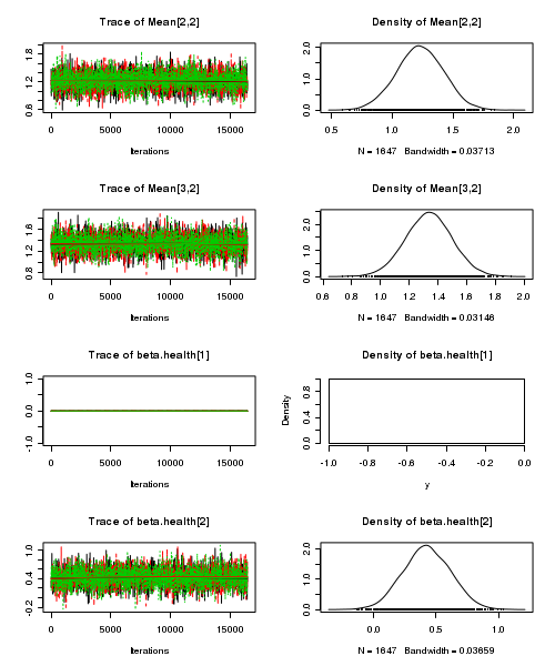
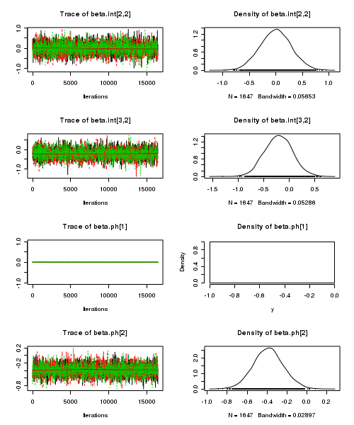
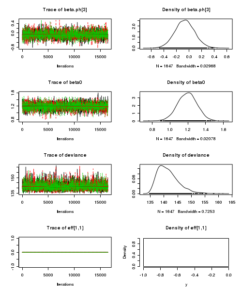
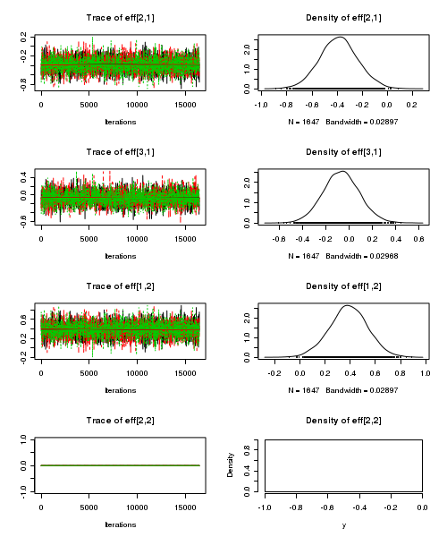
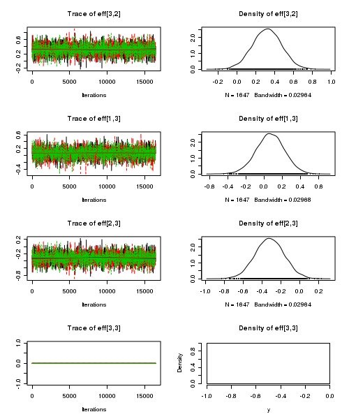
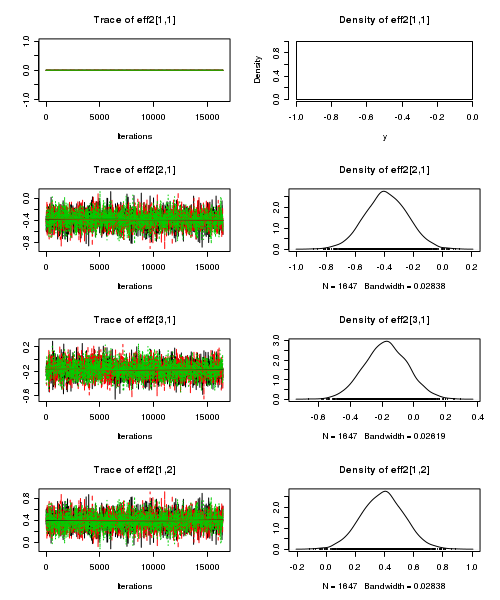
- Trace plots
View code
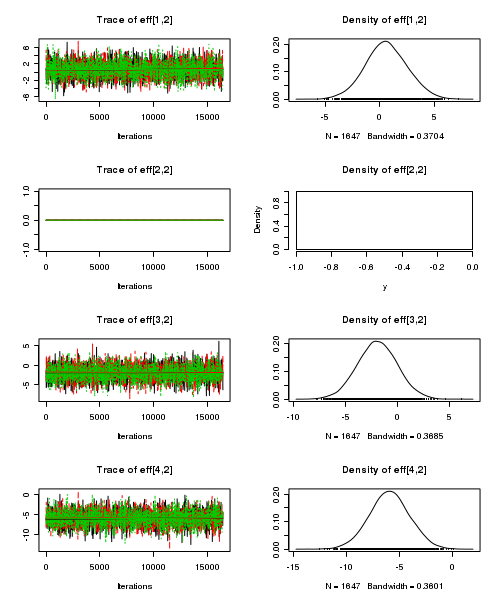
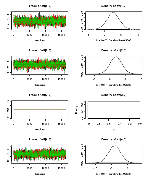
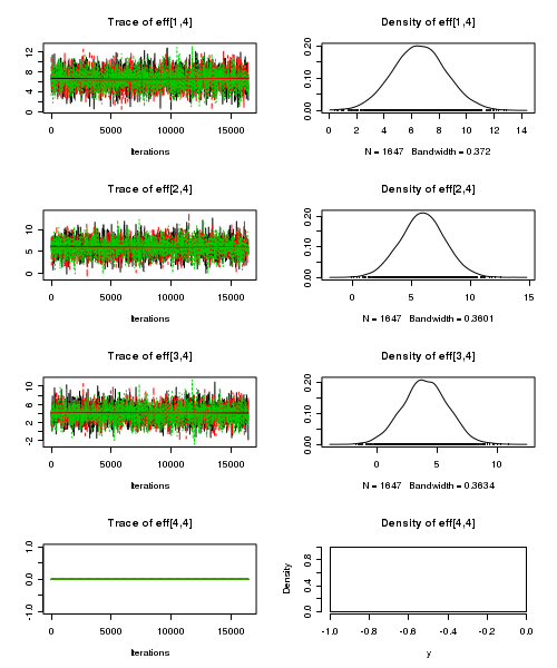
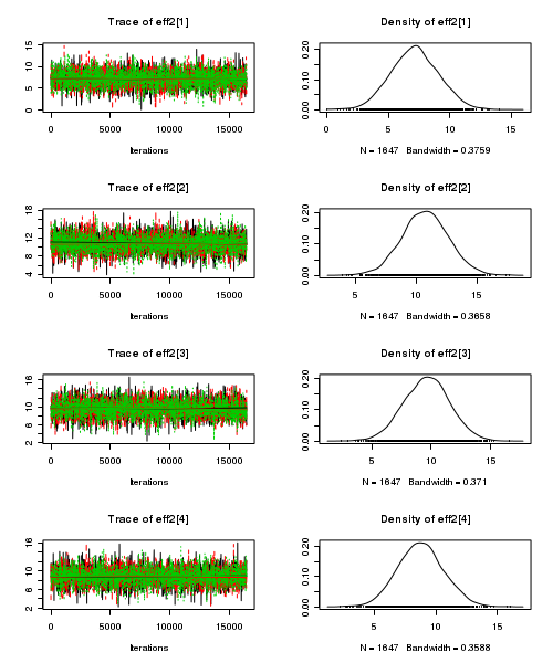
> plot(as.mcmc(starling.r2jags))
- Raftery diagnostic
View code
> raftery.diag(as.mcmc(starling.r2jags))
[[1]]

Quantile (q) = 0.025
Accuracy (r) = +/- 0.005
Probability (s) = 0.95

You need a sample size of at least 3746 with these values of q, r and s

[[2]]

Quantile (q) = 0.025
Accuracy (r) = +/- 0.005
Probability (s) = 0.95

You need a sample size of at least 3746 with these values of q, r and s

[[3]]

Quantile (q) = 0.025
Accuracy (r) = +/- 0.005
Probability (s) = 0.95

You need a sample size of at least 3746 with these values of q, r and s
- Autocorrelation
View code
> autocorr.diag(as.mcmc(starling.r2jags))
        Mean[1,1]  Mean[2,1] Mean[1,2] Mean[2,2] Mean[1,3] Mean[2,3]  Mean[1,4] Mean[2,4]
Lag 0    1.000000  1.0000000  1.000000  1.000000 1.0000000  1.000000  1.0000000  1.000000
Lag 10  -0.001908  0.0039394  0.007642 -0.003132 0.0008062 -0.009733  0.0015500  0.004218
Lag 50  -0.010543  0.0007551 -0.023796  0.007433 0.0175925 -0.017918 -0.0002732 -0.018483
Lag 100 -0.017432  0.0037170  0.011733 -0.020159 0.0175249 -0.019843  0.0045985 -0.000722
Lag 500 -0.027325 -0.0155207  0.002354 -0.007411 0.0041462  0.002988 -0.0086342  0.011634
        beta.int[1,1] beta.int[2,1] beta.int[1,2] beta.int[2,2] beta.int[1,3] beta.int[2,3]
Lag 0             NaN           NaN           NaN      1.000000           NaN      1.000000
Lag 10            NaN           NaN           NaN      0.004752           NaN      0.003448
Lag 50            NaN           NaN           NaN     -0.002842           NaN     -0.024150
Lag 100           NaN           NaN           NaN     -0.017860           NaN     -0.004386
Lag 500           NaN           NaN           NaN     -0.009378           NaN     -0.015808
        beta.int[1,4] beta.int[2,4] beta.month[1] beta.month[2] beta.situation[1] beta.situation[2]
Lag 0             NaN       1.00000           NaN     1.0000000               NaN          1.000000
Lag 10            NaN       0.01550           NaN    -0.0045391               NaN          0.007261
Lag 50            NaN       0.01528           NaN     0.0006787               NaN         -0.007635
Lag 100           NaN      -0.02872           NaN    -0.0114574               NaN          0.005118
Lag 500           NaN      -0.02084           NaN    -0.0224774               NaN         -0.003564
        beta.situation[3] beta.situation[4]     beta0   deviance eff[1,1]  eff[2,1]  eff[3,1]
Lag 0            1.000000           1.00000  1.000000  1.0000000      NaN  1.000000  1.000000
Lag 10           0.001950           0.00691 -0.001908 -0.0098722      NaN  0.007261  0.001950
Lag 50          -0.003427           0.01735 -0.010543  0.0200729      NaN -0.007635 -0.003427
Lag 100          0.004746          -0.01890 -0.017432  0.0006352      NaN  0.005118  0.004746
Lag 500         -0.019668          -0.03489 -0.027325  0.0051727      NaN -0.003564 -0.019668
        eff[4,1]  eff[1,2] eff[2,2]  eff[3,2]  eff[4,2]  eff[1,3]  eff[2,3] eff[3,3] eff[4,3]
Lag 0    1.00000  1.000000      NaN  1.000000  1.000000  1.000000  1.000000      NaN  1.00000
Lag 10   0.00691  0.007261      NaN -0.008402 -0.004394  0.001950 -0.008402      NaN  0.01358
Lag 50   0.01735 -0.007635      NaN  0.022240 -0.027287 -0.003427  0.022240      NaN  0.01526
Lag 100 -0.01890  0.005118      NaN  0.008424  0.020021  0.004746  0.008424      NaN  0.02826
Lag 500 -0.03489 -0.003564      NaN -0.019342  0.009797 -0.019668 -0.019342      NaN -0.02784
        eff[1,4]  eff[2,4] eff[3,4] eff[4,4]    eff2[1]   eff2[2]   eff2[3]   eff2[4]    sd.Int
Lag 0    1.00000  1.000000  1.00000      NaN  1.0000000  1.000000  1.000000  1.000000  1.000000
Lag 10   0.00691 -0.004394  0.01358      NaN -0.0045391  0.007980  0.008606  0.007452  0.007769
Lag 50   0.01735 -0.027287  0.01526      NaN  0.0006787 -0.001802 -0.006377 -0.016473 -0.006266
Lag 100 -0.01890  0.020021  0.02826      NaN -0.0114574 -0.006551  0.008250 -0.003164 -0.025175
Lag 500 -0.03489  0.009797 -0.02784      NaN -0.0224774 -0.015014  0.015986  0.002236  0.005423
          sd.Month  sd.Resid sd.Situation sigma.res
Lag 0    1.0000000  1.000000    1.0000000  1.000000
Lag 10  -0.0045391 -0.001852   -0.0066975 -0.002443
Lag 50   0.0006787 -0.002548    0.0002704 -0.004719
Lag 100 -0.0114574  0.002006   -0.0066467  0.004449
Lag 500 -0.0224774  0.017954   -0.0203869 -0.006040
- Trace plots
- Effects parameterization
-
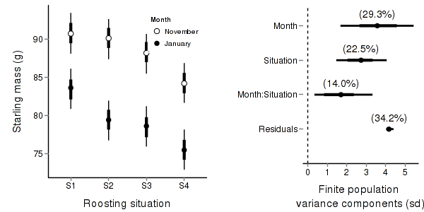
A summary figure would be nice
View code
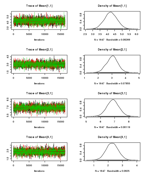
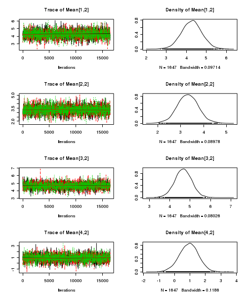
> starling.mcmc <- as.mcmc(starling.r2jags$BUGSoutput$sims.matrix)
> #get the column indexes for the parameters we are interested in
> starling.sum <- summary.mcmc(starling.mcmc, terms=c("Mean")) #or "alpha"
> starling.sum <- cbind(starling.sum, expand.grid(Month=c("November","January"), Situation=paste("S",1:4,sep="")))
>
>
> #starling.sum$name <- factor(rownames(starling.sum), levels=rownames(starling.sum))
>
> p1<-ggplot(starling.sum,aes(y=mean, x=Situation, group=Month))+
+ geom_errorbar(aes(ymin=lower, ymax=upper),width=0,size=1.5)+
+ geom_errorbar(aes(ymin=lower.1, ymax=upper.1),width=0)+
+ geom_point(aes(shape=Month, fill=Month),size=3)+
+ scale_y_continuous("Starling mass (g)")+
+ scale_x_discrete("Roosting situation")+
+ scale_shape_manual(name="Month",values=c(21,16), breaks=c("November","January"), labels=c("November","January"))+
+ scale_fill_manual(name="Month",values=c("white","black"), breaks=c("November","January"), labels=c("November","January"))+
+ murray_opts+opts(legend.position=c(1,0.99),legend.justification=c(1,1))
>
>
> #Finite-population standard deviations
> starling.sd <- summary.mcmc(starling.mcmc, terms=c("sd"))
> rownames(starling.sd) <- c("Month:Situation","Month","Residuals", "Situation")
> starling.sd$name <- factor(rownames(starling.sd), levels=c("Residuals", "Month:Situation", "Situation","Month"))
>
> p2<-ggplot(starling.sd,aes(y=name, x=median))+
+ geom_vline(xintercept=0,linetype="dashed")+
+ geom_hline(xintercept=0)+
+ scale_x_continuous("Finite population \nvariance components (sd)")+
+ geom_errorbarh(aes(xmin=lower.1, xmax=upper.1), height=0, size=1)+
+ geom_errorbarh(aes(xmin=lower, xmax=upper), height=0, size=1.5)+
+ geom_point(size=3)+
+ geom_text(aes(label=sprintf("(%4.1f%%)",Perc),vjust=-1))+
+ murray_opts+
+ opts(axis.line=theme_blank(),axis.title.y=theme_blank(),
+ axis.text.y=theme_text(size=12,hjust=1))
>
> grid.newpage()
> pushViewport(viewport(layout=grid.layout(1,2,5,5,respect=TRUE)))
> pushViewport(viewport(layout.pos.col=1, layout.pos.row=1))
> print(p1,newpage=FALSE)
> popViewport(1)
> pushViewport(viewport(layout.pos.col=2, layout.pos.row=1))
> print(p2,newpage=FALSE)
> popViewport(0)
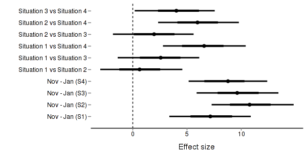
>
+
+ #eff and eff2
> starling.eff <- summary.mcmc(starling.mcmc, terms=c("eff"))
> rows <- c(matrix(upper.tri(diag(paste("S",1:4,sep=""))),ncol=1)[,1],rep(TRUE,4))
> nms <- paste("Situation",1:4)
> nms <- with(expand.grid(S1=nms, S2=nms),paste(S1,S2,sep=" vs "))
> nms <- c(nms,"Nov - Jan (S1)","Nov - Jan (S2)","Nov - Jan (S3)","Nov - Jan (S4)")
> starling.eff$name <- nms
> starling.eff <- starling.eff[rows,]
>
> p3 <- ggplot(starling.eff, aes(y=name, x=mean))+
+ geom_vline(xintercept=0,linetype="dashed")+
+ geom_hline(xintercept=0)+
+ geom_errorbarh(aes(xmin=lower.1, xmax=upper.1), height=0, size=1)+
+ geom_errorbarh(aes(xmin=lower, xmax=upper), height=0, size=1.5)+
+ geom_point(size=3)+murray_opts+
+ scale_x_continuous(name="Effect size")+
+ opts(axis.line=theme_blank(),axis.title.y=theme_blank(),
+ axis.text.y=theme_text(size=12,hjust=1))
> p3
>
+
+
+ #cohen's D
> eff<-NULL
> eff.sd <- NULL
> for (i in seq(1,7,b=2)) {
+   eff <-cbind(eff,starling.mcmc[,i] - starling.mcmc[,i+1])
+   eff.sd <- cbind(eff.sd,mean(apply(starling.mcmc[,i:(i+1)],2,sd)))
+ }
> cohen <- sweep(eff,2,eff.sd,"/")
> adply(cohen,2,function(x) {
+    data.frame(mean=mean(x), median=median(x),
+                  HPDinterval(as.mcmc(x), p=0.68), HPDinterval(as.mcmc(x)))
+ })
Error: unable to find an inherited method for function "HPDinterval", for signature "mcmc"
Unbalanced Two-factor ANOVA
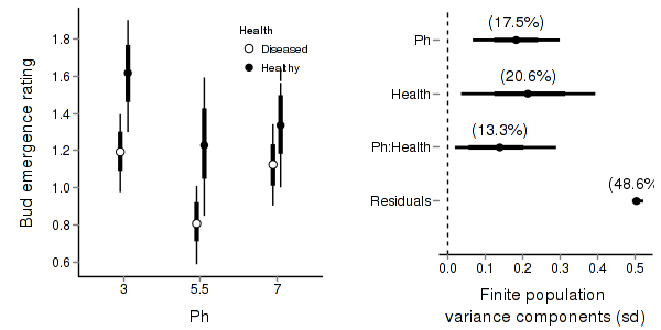
Here is a modified example from Quinn and Keough (2002). Stehman and Meredith (1995) present data from an experiment that was set up to test the hypothesis that healthy spruce seedlings break bud sooner than diseased spruce seedlings. There were 2 factors: pH (3 levels: 3, 5.5, 7) and HEALTH (2 levels: healthy, diseased). The dependent variable was the average (from 5 buds) bud emergence rating (BRATING) on each seedling. The sample size varied for each combination of pH and health, ranging from 7 to 23 seedlings. With two factors, this experiment should be analyzed with a 2 factor (2 x 3) ANOVA.
Download Stehman data set| Format of stehman.csv data files | |||||||||||||||||||||||||||||||||||||||||||||||||||||
|---|---|---|---|---|---|---|---|---|---|---|---|---|---|---|---|---|---|---|---|---|---|---|---|---|---|---|---|---|---|---|---|---|---|---|---|---|---|---|---|---|---|---|---|---|---|---|---|---|---|---|---|---|---|
|
 |
||||||||||||||||||||||||||||||||||||||||||||||||||||
Open the stehman data file.
> stehman <- read.table("../downloads/data/stehman.csv", header = T,
+     sep = ",", strip.white = T)
> head(stehman)
  PH HEALTH GROUP BRATING
1  3      D    D3     0.0
2  3      D    D3     0.8
3  3      D    D3     0.8
4  3      D    D3     0.8
5  3      D    D3     0.8
6  3      D    D3     0.8
The variable PH contains a list of pH values and is supposed to represent a factorial variable. However, because the contents of this variable are numbers, R initially treats them as numbers, and therefore considers the variable to be numeric rather than categorical. In order to force R/JAGS to treat this variable as a factor (categorical) it must be in categorical form (yet as numbers). Confused? What this means, is that to be treated as a factor, its levels must be indices and therefore the PH variable needs to be converted into a factor before being converted to a numeric. That way the levels 3, 5.5 and 7 will be coded as 1, 2 and 3.
Exploratory data analysis did not reveal any issues with normality or homogeneity of variance.
- Fit the JAGS model including all pairwise comparisons AND (just because we can), compare the bare surfaces to the surfaces with an algal biofilm. Use with either:
- Effects parameterization
bratingi = β0 + β1j(i)*phi + β2j(i)*healthi + β3j(i)*phi*healthi + εi where ε ∼ N(0,σ2)View full code> modelString=" model { #Likelihood for (i in 1:n) { brating[i]~dnorm(mean[i],tau.res) mean[i] <- beta0+beta.ph[ph[i]]+beta.health[health[i]]+ beta.int[ph[i],health[i]] y.err[i] <- brating[i] - mean[i] } #Priors and derivatives beta0 ~ dnorm(0,1.0E-6) beta.ph[1] <- 0 beta.int[1,1] <- 0 for (i in 2:nPh) { beta.ph[i] ~ dnorm(0.001, 1.0E-6) #prior beta.int[i,1] <- 0 } beta.health[1] <- 0 for (i in 2:nHealth){ beta.health[i] ~ dnorm(0.001, 1.0E-6) #prior cannot be 0, or else will have an ##init of zero and then will be dividing by zero when calculating cohen's D beta.int[1,i] <- 0 } for (i in 2:nPh) { for (j in 2:nHealth){ beta.int[i,j] ~ dnorm(0, 1.0E-6) } } #Means for (i in 1:nPh) { for (j in 1:nHealth) { Mean[i,j] <- beta0 + beta.ph[i] + beta.health[j] + beta.int[i,j] } } sigma.res ~ dgamma(0.001, 0.001) #prior on sd residuals tau.res <- 1 / (sigma.res * sigma.res) sd.Ph <- sd(beta.ph[]) sd.Health <- sd(beta.health[]) sd.Int <- sd(beta.int[,]) sd.Resid <- sd(y.err[]) #Pairwise comparisons of PH for (i in 1:nPh) { for (j in 1:nPh) { eff[i,j] <- (beta.ph[i] - beta.ph[j]) eff2[i,j] <- ((Mean[i,1]+Mean[i,2])/2) - ((Mean[j,1]+Mean[j,2])/2) } } # #Effects of ph within each health # for (i in 1:nHealth) { # eff2[i] <- Mean[1,i] - Mean[2,i] # } } " > ## write the model to a text file (I suggest you alter the path to somewhere more relevant > ## to your system!) > writeLines(modelString,con="../downloads/BUGSscripts/ws9.6bQ2.1a.txt") > stehman.list <- with(stehman, + list(brating=BRATING, + ph=as.numeric(as.factor(PH)), health=as.numeric(HEALTH), + n=nrow(stehman), nPh=length(levels(as.factor(PH))), + nHealth=length(levels(HEALTH)) + ) + ) > > params <- c("beta0","beta.ph","beta.health","beta.int","sigma.res","sd.Ph","sd.Health","sd.Int","sd.Resid", "Mean","eff","eff2") > #params <- c("beta0","beta.ph","beta.health","beta.int","sigma.res","Mean", "sd.Ph","sd.Health","sd.Int","sd.Resid", "eff","eff2") > > adaptSteps = 1000 > burnInSteps = 200 > nChains = 3 > numSavedSteps = 5000 > thinSteps = 10 > nIter = ceiling((numSavedSteps * thinSteps)/nChains) > > library(R2jags) > ## > stehman.r2jags <- jags(data=stehman.list, + inits=NULL, #or inits=list(inits,inits,inits) # since there are three chains + parameters.to.save=params, + model.file="../downloads/BUGSscripts/ws9.6bQ2.1a.txt", + n.chains=3, + n.iter=nIter, + n.burnin=burnInSteps, + n.thin=thinSteps + )
Compiling model graph
   Resolving undeclared variables
   Allocating nodes
   Graph Size: 385

Initializing model
> print(stehman.r2jags)
Inference for Bugs model at "../downloads/BUGSscripts/ws9.6bQ2.1a.txt", fit using jags, 3 chains, each with 16667 iterations (first 200 discarded), n.thin = 10 n.sims = 4941 iterations saved mu.vect sd.vect 2.5% 25% 50% 75% 97.5% Rhat n.eff Mean[1,1] 1.193 0.107 0.979 1.120 1.194 1.266 1.400 1.001 2700 Mean[2,1] 0.807 0.107 0.592 0.735 0.807 0.879 1.016 1.001 3400 Mean[3,1] 1.125 0.112 0.905 1.050 1.124 1.199 1.348 1.001 4900 Mean[1,2] 1.618 0.156 1.311 1.516 1.616 1.725 1.920 1.001 4900 Mean[2,2] 1.229 0.192 0.849 1.099 1.228 1.359 1.597 1.002 2100 Mean[3,2] 1.337 0.163 1.012 1.228 1.337 1.447 1.656 1.002 2200 beta.health[1] 0.000 0.000 0.000 0.000 0.000 0.000 0.000 1.000 1 beta.health[2] 0.425 0.189 0.059 0.299 0.425 0.556 0.796 1.002 2400 beta.int[1,1] 0.000 0.000 0.000 0.000 0.000 0.000 0.000 1.000 1 beta.int[2,1] 0.000 0.000 0.000 0.000 0.000 0.000 0.000 1.000 1 beta.int[3,1] 0.000 0.000 0.000 0.000 0.000 0.000 0.000 1.000 1 beta.int[1,2] 0.000 0.000 0.000 0.000 0.000 0.000 0.000 1.000 1 beta.int[2,2] -0.003 0.292 -0.561 -0.201 -0.001 0.195 0.573 1.001 2600 beta.int[3,2] -0.214 0.273 -0.738 -0.399 -0.211 -0.028 0.333 1.002 1600 beta.ph[1] 0.000 0.000 0.000 0.000 0.000 0.000 0.000 1.000 1 beta.ph[2] -0.386 0.152 -0.683 -0.488 -0.387 -0.288 -0.081 1.001 4900 beta.ph[3] -0.068 0.156 -0.374 -0.172 -0.069 0.034 0.246 1.001 4700 beta0 1.193 0.107 0.979 1.120 1.194 1.266 1.400 1.001 2700 eff[1,1] 0.000 0.000 0.000 0.000 0.000 0.000 0.000 1.000 1 eff[2,1] -0.386 0.152 -0.683 -0.488 -0.387 -0.288 -0.081 1.001 4900 eff[3,1] -0.068 0.156 -0.374 -0.172 -0.069 0.034 0.246 1.001 4700 eff[1,2] 0.386 0.152 0.081 0.288 0.387 0.488 0.683 1.001 4900 eff[2,2] 0.000 0.000 0.000 0.000 0.000 0.000 0.000 1.000 1 eff[3,2] 0.318 0.153 0.013 0.215 0.320 0.423 0.621 1.001 4900 eff[1,3] 0.068 0.156 -0.246 -0.034 0.069 0.172 0.374 1.001 4700 eff[2,3] -0.318 0.153 -0.621 -0.423 -0.320 -0.215 -0.013 1.001 4900 eff[3,3] 0.000 0.000 0.000 0.000 0.000 0.000 0.000 1.000 1 eff2[1,1] 0.000 0.000 0.000 0.000 0.000 0.000 0.000 1.000 1 eff2[2,1] -0.388 0.147 -0.676 -0.486 -0.389 -0.289 -0.099 1.001 4900 eff2[3,1] -0.175 0.135 -0.442 -0.265 -0.175 -0.083 0.091 1.001 4900 eff2[1,2] 0.388 0.147 0.099 0.289 0.389 0.486 0.676 1.001 4900 eff2[2,2] 0.000 0.000 0.000 0.000 0.000 0.000 0.000 1.000 1 eff2[3,2] 0.213 0.149 -0.072 0.114 0.213 0.313 0.504 1.001 4900 eff2[1,3] 0.175 0.135 -0.091 0.083 0.175 0.265 0.442 1.001 4900 eff2[2,3] -0.213 0.149 -0.504 -0.313 -0.213 -0.114 0.072 1.001 4900 eff2[3,3] 0.000 0.000 0.000 0.000 0.000 0.000 0.000 1.000 1 sd.Health 0.214 0.093 0.036 0.150 0.212 0.278 0.398 1.004 1500 sd.Int 0.145 0.074 0.027 0.090 0.137 0.193 0.310 1.001 4900 sd.Ph 0.181 0.059 0.064 0.141 0.181 0.220 0.297 1.001 4900 sd.Resid 0.504 0.009 0.492 0.498 0.502 0.509 0.525 1.001 4900 sigma.res 0.512 0.039 0.442 0.484 0.509 0.537 0.595 1.001 4900 deviance 141.478 3.856 135.933 138.589 140.846 143.614 150.620 1.001 4900 For each parameter, n.eff is a crude measure of effective sample size, and Rhat is the potential scale reduction factor (at convergence, Rhat=1). DIC info (using the rule, pD = var(deviance)/2) pD = 7.4 and DIC = 148.9 DIC is an estimate of expected predictive error (lower deviance is better). - Means parameterization
bratingi = αj(i)*phi*healthi + εi where ε ∼ N(0,σ2)View full code
> modelString="
model {
   #Likelihood
   for (i in 1:n) {
      brating[i]~dnorm(mean[i],tau.res)
      mean[i] <- alpha[ph[i],health[i]]
      y.err[i] <- brating[i] - mean[i]
   }

   #Priors and derivatives
   for (i in 1:nPh) {
     for (j in 1:nHealth){
       alpha[i,j] ~ dnorm(0, 1.0E-6)
     }
   }

   sigma.res ~ dgamma(0.001, 0.001) #prior on sd residuals
   tau.res <- 1 / (sigma.res * sigma.res)

   #Effects
   beta0 <- alpha[1,1]
   for (i in 1:nPh) {
     beta.ph[i] <- alpha[i,1]-beta0
   }
   for (i in 1:nHealth) {
     beta.health[i] <- alpha[1,i]-beta0
   }

   for (i in 1:nPh) {
     for (j in 1:nHealth) {
	   beta.int[i,j] <- alpha[i,j]-beta.ph[i]-beta.health[j]-beta0
	 }
   }
   sd.Ph <- sd(beta.ph[])
   sd.Health <- sd(beta.health[])
   sd.Int <- sd(beta.int[,])
   sd.Resid <- sd(y.err[])

   #Pairwise comparisons of PH
   for (i in 1:nPh) {
     for (j in 1:nPh) {
	   eff[i,j] <- (beta.ph[i] - beta.ph[j])
       eff2[i,j] <- ((alpha[i,1]+alpha[i,2])/2) - ((alpha[j,1]+alpha[j,2])/2)
	 }
   }
 }
"
> ## write the model to a text file (I suggest you alter the path to somewhere more relevant
> ## to your system!)
> writeLines(modelString,con="../downloads/BUGSscripts/ws9.6bQ2.1b.txt")
> stehman.list <- with(stehman,
+                          list(brating=BRATING,
+                          ph=as.numeric(as.factor(PH)), health=as.numeric(HEALTH),
+                                  n=nrow(stehman), nPh=length(levels(as.factor(PH))),
+                                  nHealth=length(levels(HEALTH))
+                         )
+            )
>
> params <- c("beta.ph","beta.health","beta.int","sigma.res","sd.Ph","sd.Health","sd.Int","sd.Resid","eff","eff2")
> adaptSteps = 1000
> burnInSteps = 200
> nChains = 3
> numSavedSteps = 5000
> thinSteps = 10
> nIter = ceiling((numSavedSteps * thinSteps)/nChains)
>
> library(R2jags)
> ##
> stehman.r2jags2 <- jags(data=stehman.list,
+           inits=NULL, #or inits=list(inits,inits,inits) # since there are three chains
+           parameters.to.save=params,
+           model.file="../downloads/BUGSscripts/ws9.6bQ2.1b.txt",
+           n.chains=3,
+           n.iter=nIter,
+           n.burnin=burnInSteps,
+       n.thin=thinSteps
+           )
Compiling model graph
   Resolving undeclared variables
   Allocating nodes
   Graph Size: 395

Initializing model
> print(stehman.r2jags2)
Inference for Bugs model at "../downloads/BUGSscripts/ws9.6bQ2.1b.txt", fit using jags,
 3 chains, each with 16667 iterations (first 200 discarded), n.thin = 10
 n.sims = 4941 iterations saved
               mu.vect sd.vect    2.5%     25%     50%     75%   97.5%  Rhat n.eff
beta.health[1]   0.000   0.000   0.000   0.000   0.000   0.000   0.000 1.000     1
beta.health[2]   0.430   0.186   0.070   0.305   0.427   0.556   0.791 1.001  4900
beta.int[1,1]    0.000   0.000   0.000   0.000   0.000   0.000   0.000 1.000     1
beta.int[2,1]    0.000   0.000   0.000   0.000   0.000   0.000   0.000 1.000     1
beta.int[3,1]    0.000   0.000   0.000   0.000   0.000   0.000   0.000 1.000     1
beta.int[1,2]    0.000   0.000   0.000   0.000   0.000   0.000   0.000 1.000     1
beta.int[2,2]   -0.008   0.288  -0.581  -0.195  -0.010   0.183   0.556 1.001  4900
beta.int[3,2]   -0.215   0.267  -0.739  -0.390  -0.219  -0.034   0.294 1.001  4900
beta.ph[1]       0.000   0.000   0.000   0.000   0.000   0.000   0.000 1.000     1
beta.ph[2]      -0.382   0.151  -0.677  -0.483  -0.382  -0.280  -0.083 1.001  4900
beta.ph[3]      -0.067   0.154  -0.368  -0.169  -0.066   0.038   0.233 1.001  4900
eff[1,1]         0.000   0.000   0.000   0.000   0.000   0.000   0.000 1.000     1
eff[2,1]        -0.382   0.151  -0.677  -0.483  -0.382  -0.280  -0.083 1.001  4900
eff[3,1]        -0.067   0.154  -0.368  -0.169  -0.066   0.038   0.233 1.001  4900
eff[1,2]         0.382   0.151   0.083   0.280   0.382   0.483   0.677 1.001  4900
eff[2,2]         0.000   0.000   0.000   0.000   0.000   0.000   0.000 1.000     1
eff[3,2]         0.315   0.153   0.017   0.211   0.316   0.417   0.617 1.001  4900
eff[1,3]         0.067   0.154  -0.233  -0.038   0.066   0.169   0.368 1.001  4900
eff[2,3]        -0.315   0.153  -0.617  -0.417  -0.316  -0.211  -0.017 1.001  4900
eff[3,3]         0.000   0.000   0.000   0.000   0.000   0.000   0.000 1.000     1
eff2[1,1]        0.000   0.000   0.000   0.000   0.000   0.000   0.000 1.000     1
eff2[2,1]       -0.386   0.146  -0.674  -0.485  -0.384  -0.286  -0.101 1.001  4900
eff2[3,1]       -0.174   0.136  -0.442  -0.266  -0.173  -0.083   0.087 1.001  3700
eff2[1,2]        0.386   0.146   0.101   0.286   0.384   0.485   0.674 1.001  4900
eff2[2,2]        0.000   0.000   0.000   0.000   0.000   0.000   0.000 1.000     1
eff2[3,2]        0.212   0.147  -0.072   0.110   0.213   0.309   0.498 1.001  2600
eff2[1,3]        0.174   0.136  -0.087   0.083   0.173   0.266   0.442 1.001  3700
eff2[2,3]       -0.212   0.147  -0.498  -0.309  -0.213  -0.110   0.072 1.001  2600
eff2[3,3]        0.000   0.000   0.000   0.000   0.000   0.000   0.000 1.000     1
sd.Health        0.216   0.091   0.039   0.153   0.213   0.278   0.396 1.002  4700
sd.Int           0.143   0.074   0.027   0.089   0.136   0.189   0.307 1.001  3200
sd.Ph            0.179   0.059   0.067   0.138   0.179   0.218   0.296 1.001  4900
sd.Resid         0.504   0.009   0.493   0.498   0.502   0.508   0.526 1.001  4900
sigma.res        0.511   0.038   0.442   0.484   0.509   0.536   0.593 1.001  4900
deviance       141.377   3.820 135.963 138.571 140.734 143.466 150.632 1.001  4900

For each parameter, n.eff is a crude measure of effective sample size,
and Rhat is the potential scale reduction factor (at convergence, Rhat=1).

DIC info (using the rule, pD = var(deviance)/2)
pD = 7.3 and DIC = 148.7
DIC is an estimate of expected predictive error (lower deviance is better).
- Effects parameterization
- Before fully exploring the parameters, it is prudent to examine the convergence and mixing diagnostics.
Chose either the effects or means parameterization model (they should yield much the same).
- Trace plots
View code
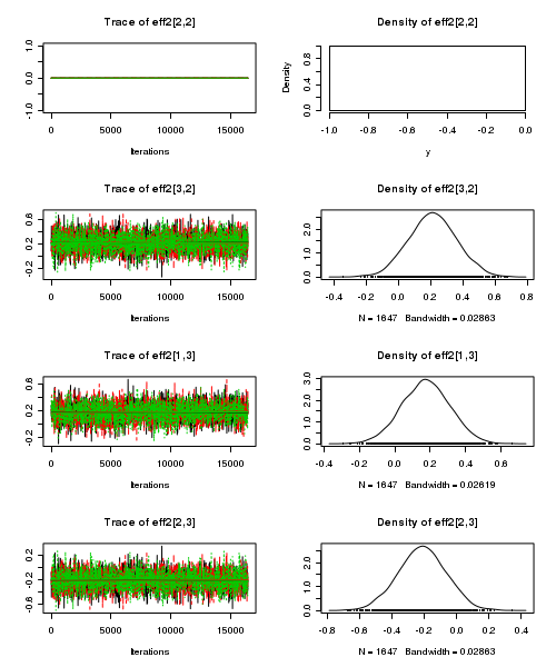
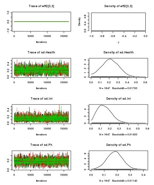
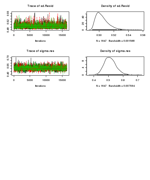
> plot(as.mcmc(stehman.r2jags))
- Raftery diagnostic
View code
> raftery.diag(as.mcmc(stehman.r2jags))
[[1]]

Quantile (q) = 0.025
Accuracy (r) = +/- 0.005
Probability (s) = 0.95

You need a sample size of at least 3746 with these values of q, r and s

[[2]]

Quantile (q) = 0.025
Accuracy (r) = +/- 0.005
Probability (s) = 0.95

You need a sample size of at least 3746 with these values of q, r and s

[[3]]

Quantile (q) = 0.025
Accuracy (r) = +/- 0.005
Probability (s) = 0.95

You need a sample size of at least 3746 with these values of q, r and s
- Autocorrelation
View code
> autocorr.diag(as.mcmc(stehman.r2jags))
        Mean[1,1] Mean[2,1] Mean[3,1] Mean[1,2]  Mean[2,2] Mean[3,2] beta.health[1] beta.health[2]
Lag 0    1.000000   1.00000  1.000000  1.000000  1.0000000  1.000000            NaN       1.000000
Lag 10   0.015825  -0.02483  0.029052  0.001061 -0.0204654 -0.025140            NaN      -0.007364
Lag 50  -0.014374  -0.02767  0.003399  0.035938 -0.0004691 -0.003156            NaN      -0.002253
Lag 100  0.008493  -0.01021 -0.007150  0.018119 -0.0403369 -0.006234            NaN       0.003267
Lag 500  0.016258   0.02617 -0.019063  0.022172 -0.0003144  0.010743            NaN       0.016014
        beta.int[1,1] beta.int[2,1] beta.int[3,1] beta.int[1,2] beta.int[2,2] beta.int[3,2]
Lag 0             NaN           NaN           NaN           NaN      1.000000      1.000000
Lag 10            NaN           NaN           NaN           NaN      0.006026     -0.002851
Lag 50            NaN           NaN           NaN           NaN      0.007103      0.000095
Lag 100           NaN           NaN           NaN           NaN     -0.006275     -0.012467
Lag 500           NaN           NaN           NaN           NaN      0.007731      0.003171
        beta.ph[1] beta.ph[2] beta.ph[3]     beta0  deviance eff[1,1]  eff[2,1]  eff[3,1]  eff[1,2]
Lag 0          NaN   1.000000   1.000000  1.000000  1.000000      NaN  1.000000  1.000000  1.000000
Lag 10         NaN   0.005331   0.014305  0.015825 -0.006270      NaN  0.005331  0.014305  0.005331
Lag 50         NaN  -0.041872  -0.023950 -0.014374 -0.005720      NaN -0.041872 -0.023950 -0.041872
Lag 100        NaN  -0.004293   0.001759  0.008493 -0.001357      NaN -0.004293  0.001759 -0.004293
Lag 500        NaN   0.032709   0.003853  0.016258 -0.025478      NaN  0.032709  0.003853  0.032709
        eff[2,2]  eff[3,2]  eff[1,3]  eff[2,3] eff[3,3] eff2[1,1] eff2[2,1] eff2[3,1] eff2[1,2]
Lag 0        NaN  1.000000  1.000000  1.000000      NaN       NaN   1.00000  1.000000   1.00000
Lag 10       NaN -0.001814  0.014305 -0.001814      NaN       NaN  -0.02276  0.008053  -0.02276
Lag 50       NaN -0.022216 -0.023950 -0.022216      NaN       NaN   0.02488  0.008395   0.02488
Lag 100      NaN -0.014981  0.001759 -0.014981      NaN       NaN  -0.02791  0.009600  -0.02791
Lag 500      NaN  0.012182  0.003853  0.012182      NaN       NaN   0.01505  0.031804   0.01505
        eff2[2,2] eff2[3,2] eff2[1,3] eff2[2,3] eff2[3,3] sd.Health    sd.Int      sd.Ph  sd.Resid
Lag 0         NaN   1.00000  1.000000   1.00000       NaN  1.000000  1.000000  1.000e+00  1.000000
Lag 10        NaN  -0.03517  0.008053  -0.03517       NaN -0.007974 -0.007266  4.519e-05 -0.020409
Lag 50        NaN  -0.01782  0.008395  -0.01782       NaN  0.001795  0.006918 -2.808e-02 -0.013002
Lag 100       NaN  -0.02574  0.009600  -0.02574       NaN  0.001555 -0.025238 -1.349e-02  0.005629
Lag 500       NaN   0.01089  0.031804   0.01089       NaN  0.018169 -0.003348  3.505e-02 -0.042728
        sigma.res
Lag 0   1.0000000
Lag 10  0.0120803
Lag 50  0.0134666
Lag 100 0.0007495
Lag 500 0.0017084
- Trace plots
-
A summary figure would be nice
View code
> stehman.mcmc <- as.mcmc(stehman.r2jags$BUGSoutput$sims.matrix)
> #get the column indexes for the parameters we are interested in
> stehman.sum <- summary.mcmc(stehman.mcmc, terms=c("Mean")) #or "alpha"
> stehman.sum <- cbind(stehman.sum, expand.grid(Ph=c("3","5.5","7"), Health=c("Diseased","Healthy")))
>
>
> p1<-ggplot(stehman.sum,aes(y=mean, x=Ph, group=Health))+
+ geom_errorbar(aes(ymin=lower, ymax=upper),width=0,size=1.5,position=position_dodge(0.2))+
+ geom_errorbar(aes(ymin=lower.1, ymax=upper.1),width=0,position=position_dodge(0.2))+
+ geom_point(aes(shape=Health, fill=Health),size=3,position=position_dodge(0.2))+
+ scale_y_continuous("Bud emergence rating")+
+ scale_x_discrete("Ph")+
+ scale_shape_manual(name="Health",values=c(21,16), breaks=c("Diseased","Healthy"), labels=c("Diseased","Healthy"))+
+ scale_fill_manual(name="Health",values=c("white","black"), breaks=c("Diseased","Healthy"), labels=c("Diseased","Healthy"))+
+ murray_opts+opts(legend.position=c(1,0.99),legend.justification=c(1,1))
>
>
> #Finite-population standard deviations
> stehman.sd <- summary.mcmc(stehman.mcmc, terms=c("sd"))
> rownames(stehman.sd) <- c("Health","Ph:Health","Ph", "Residuals")
> stehman.sd$name <- factor(c("Health","Ph:Health","Ph", "Residuals"), levels=c("Residuals", "Ph:Health", "Health","Ph"))
>
> p2<-ggplot(stehman.sd,aes(y=name, x=median))+
+ geom_vline(xintercept=0,linetype="dashed")+
+ geom_hline(xintercept=0)+
+ scale_x_continuous("Finite population \nvariance components (sd)")+
+ geom_errorbarh(aes(xmin=lower.1, xmax=upper.1), height=0, size=1)+
+ geom_errorbarh(aes(xmin=lower, xmax=upper), height=0, size=1.5)+
+ geom_point(size=3)+
+ geom_text(aes(label=sprintf("(%4.1f%%)",Perc),vjust=-1))+
+ murray_opts+
+ opts(axis.line=theme_blank(),axis.title.y=theme_blank(),
+ axis.text.y=theme_text(size=12,hjust=1))
>
> grid.newpage()
> pushViewport(viewport(layout=grid.layout(1,2,5,5,respect=TRUE)))
> pushViewport(viewport(layout.pos.col=1, layout.pos.row=1))
> print(p1,newpage=FALSE)
> popViewport(1)
> pushViewport(viewport(layout.pos.col=2, layout.pos.row=1))
> print(p2,newpage=FALSE)
> popViewport(0)
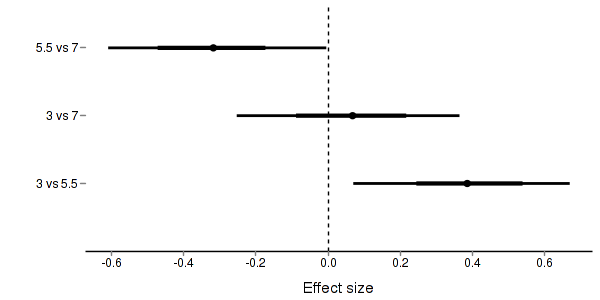
>
+
+ #eff and eff2
> stehman.eff <- summary.mcmc(stehman.mcmc, terms=c("eff\\["))
> rows <- matrix(upper.tri(diag(c("3","5.5","7"))),ncol=1)[,1]
> #rows <- c(matrix(upper.tri(diag(c("3","5.5","7"))),ncol=1)[,1],
> #matrix(upper.tri(diag(c("3","5.5","7"))),ncol=1)[,1]
> #)
> nms <- c("3","5.5","7")
> nms <- with(expand.grid(S1=nms, S2=nms),paste(S1,S2,sep=" vs "))
> #nms <- c(nms,nms)
> stehman.eff$name <- nms
> stehman.eff <- stehman.eff[rows,]
>
> p3 <- ggplot(stehman.eff, aes(y=name, x=mean))+
+ geom_vline(xintercept=0,linetype="dashed")+
+ geom_hline(xintercept=0)+
+ geom_errorbarh(aes(xmin=lower.1, xmax=upper.1), height=0, size=1)+
+ geom_errorbarh(aes(xmin=lower, xmax=upper), height=0, size=1.5)+
+ geom_point(size=3)+murray_opts+
+ scale_x_continuous(name="Effect size")+
+ opts(axis.line=theme_blank(),axis.title.y=theme_blank(),
+ axis.text.y=theme_text(size=12,hjust=1))
> p3
>
+
+
+ #cohen's D
> eff<-NULL
> eff.sd <- NULL
> for (i in seq(1,7,b=2)) {
+   eff <-cbind(eff,stehman.mcmc[,i] - stehman.mcmc[,i+1])
+   eff.sd <- cbind(eff.sd,mean(apply(stehman.mcmc[,i:(i+1)],2,sd)))
+ }
> cohen <- sweep(eff,2,eff.sd,"/")
> adply(cohen,2,function(x) {
+    data.frame(mean=mean(x), median=median(x),
+                  HPDinterval(as.mcmc(x), p=0.68), HPDinterval(as.mcmc(x)))
+ })
Error: unable to find an inherited method for function "HPDinterval", for signature "mcmc"
Two-factor ANOVA with substantial interactions
An ecologist studying a rocky shore at Phillip Island, in southeastern Australia, was interested in how clumps of intertidal mussels are maintained. In particular, he wanted to know how densities of adult mussels affected recruitment of young individuals from the plankton. As with most marine invertebrates, recruitment is highly patchy in time, so he expected to find seasonal variation, and the interaction between season and density - whether effects of adult mussel density vary across seasons - was the aspect of most interest.
The data were collected from four seasons, and with two densities of adult mussels. The experiment consisted of clumps of adult mussels attached to the rocks. These clumps were then brought back to the laboratory, and the number of baby mussels recorded. There were 3-6 replicate clumps for each density and season combination.
Download Quinn data set| Format of quinn.csv data files | ||||||||||||||||||||||||||||||||||||||||||||||||||||||||||||||||||
|---|---|---|---|---|---|---|---|---|---|---|---|---|---|---|---|---|---|---|---|---|---|---|---|---|---|---|---|---|---|---|---|---|---|---|---|---|---|---|---|---|---|---|---|---|---|---|---|---|---|---|---|---|---|---|---|---|---|---|---|---|---|---|---|---|---|---|
|
 |
Open the quinn data file.
> quinn <- read.table("../downloads/data/quinn.csv", header = T, sep = ",",
+     strip.white = T)
> head(quinn)
  SEASON DENSITY RECRUITS SQRTRECRUITS      GROUP
1 Spring     Low       15        3.873  SpringLow
2 Spring     Low       10        3.162  SpringLow
3 Spring     Low       13        3.606  SpringLow
4 Spring     Low       13        3.606  SpringLow
5 Spring     Low        5        2.236  SpringLow
6 Spring    High       11        3.317 SpringHigh
Exploratory data analysis revealed non-normality and heterogeneous variances (probably due to non-normality). As the response is count data, a square-root transformation is one possible way of addressing these issues.
- Fit the JAGS model including all pairwise comparisons AND (just because we can), compare the bare surfaces to the surfaces with an algal biofilm. Use with either:
- Effects parameterization
recruitsi = β0 + β1j(i)*seasoni + β2j(i)*densityi + β3j(i)*seasoni*densityi + εi where ε ∼ N(0,σ2)View full code> modelString=" data { srecruits <- sqrt(recruits) } model { #Likelihood for (i in 1:n) { srecruits[i]~dnorm(mean[i],tau.res) mean[i] <- beta0+beta.season[season[i]]+beta.density[density[i]]+ beta.int[season[i],density[i]] y.err[i] <- srecruits[i] - mean[i] } #Priors and derivatives beta0 ~ dnorm(0,1.0E-6) beta.season[1] <- 0 beta.int[1,1] <- 0 for (i in 2:nSeason) { beta.season[i] ~ dnorm(0, 1.0E-6) #prior beta.int[i,1] <- 0 } beta.density[1] <- 0 for (i in 2:nDensity){ beta.density[i] ~ dnorm(0, 1.0E-6) #prior cannot be 0, or else will have an beta.int[1,i] <- 0 } for (i in 2:nSeason) { for (j in 2:nDensity){ beta.int[i,j] ~ dnorm(0, 1.0E-6) } } #Means for (i in 1:nSeason) { for (j in 1:nDensity) { Mean[i,j] <- beta0 + beta.season[i] + beta.density[j] + beta.int[i,j] } } sigma.res ~ dgamma(0.001, 0.001) #prior on sd residuals tau.res <- 1 / (sigma.res * sigma.res) sd.Season <- sd(beta.season[]) sd.Density <- sd(beta.density[]) sd.Int <- sd(beta.int[,]) sd.Resid <- sd(y.err[]) #Pairwise comparisons of Density (in each Season) for (i in 1:nSeason) { eff[i] <- Mean[i,1] - Mean[i,2] } } " > ## write the model to a text file (I suggest you alter the path to somewhere more relevant > ## to your system!) > writeLines(modelString,con="../downloads/BUGSscripts/ws9.6bQ3.1a.txt") > quinn.list <- with(quinn, + list(recruits=RECRUITS, + season=as.numeric(SEASON), density=as.numeric(DENSITY), + n=nrow(quinn), nSeason=length(levels(SEASON)), + nDensity=length(levels(DENSITY)) + ) + ) > > #params <- c("beta0","beta.season","beta.density","beta.int","sigma.res","sd.Season","sd.Density","sd.Int","sd.Resid", "Mean","eff","eff2") > params <- c("beta0","beta.season","beta.density","beta.int","sigma.res","Mean", "sd.Season","sd.Density","sd.Int","sd.Resid","eff") > > adaptSteps = 1000 > burnInSteps = 200 > nChains = 3 > numSavedSteps = 5000 > thinSteps = 10 > nIter = ceiling((numSavedSteps * thinSteps)/nChains) > > library(R2jags) > ## > quinn.r2jags <- jags(data=quinn.list, + inits=NULL, #or inits=list(inits,inits,inits) # since there are three chains + parameters.to.save=params, + model.file="../downloads/BUGSscripts/ws9.6bQ3.1a.txt", + n.chains=3, + n.iter=nIter, + n.burnin=burnInSteps, + n.thin=thinSteps + )
Compiling data graph
   Resolving undeclared variables
   Allocating nodes
   Initializing
   Reading data back into data table
Compiling model graph
   Resolving undeclared variables
   Allocating nodes
   Graph Size: 249

Initializing model
> print(quinn.r2jags)
Inference for Bugs model at "../downloads/BUGSscripts/ws9.6bQ3.1a.txt", fit using jags, 3 chains, each with 16667 iterations (first 200 discarded), n.thin = 10 n.sims = 4941 iterations saved mu.vect sd.vect 2.5% 25% 50% 75% 97.5% Rhat n.eff Mean[1,1] 4.232 0.430 3.409 3.947 4.227 4.520 5.075 1.001 4900 Mean[2,1] 3.023 0.423 2.182 2.752 3.034 3.296 3.857 1.001 4900 Mean[3,1] 6.875 0.430 6.027 6.591 6.877 7.153 7.727 1.001 4900 Mean[4,1] 2.272 0.427 1.437 1.987 2.267 2.559 3.114 1.002 1400 Mean[1,2] 4.264 0.515 3.241 3.927 4.271 4.600 5.275 1.002 1100 Mean[2,2] 3.309 0.465 2.384 2.994 3.308 3.616 4.255 1.001 4900 Mean[3,2] 4.658 0.421 3.820 4.379 4.659 4.935 5.477 1.001 4900 Mean[4,2] 0.925 0.613 -0.318 0.516 0.941 1.338 2.096 1.001 4900 beta.density[1] 0.000 0.000 0.000 0.000 0.000 0.000 0.000 1.000 1 beta.density[2] 0.032 0.672 -1.260 -0.418 0.037 0.484 1.340 1.002 1700 beta.int[1,1] 0.000 0.000 0.000 0.000 0.000 0.000 0.000 1.000 1 beta.int[2,1] 0.000 0.000 0.000 0.000 0.000 0.000 0.000 1.000 1 beta.int[3,1] 0.000 0.000 0.000 0.000 0.000 0.000 0.000 1.000 1 beta.int[4,1] 0.000 0.000 0.000 0.000 0.000 0.000 0.000 1.000 1 beta.int[1,2] 0.000 0.000 0.000 0.000 0.000 0.000 0.000 1.000 1 beta.int[2,2] 0.254 0.914 -1.562 -0.348 0.250 0.863 2.062 1.002 2300 beta.int[3,2] -2.249 0.911 -4.056 -2.839 -2.253 -1.670 -0.413 1.001 4400 beta.int[4,2] -1.379 0.994 -3.298 -2.044 -1.380 -0.713 0.578 1.002 1200 beta.season[1] 0.000 0.000 0.000 0.000 0.000 0.000 0.000 1.000 1 beta.season[2] -1.209 0.603 -2.402 -1.620 -1.209 -0.814 -0.040 1.001 4900 beta.season[3] 2.643 0.610 1.437 2.225 2.658 3.047 3.845 1.001 4900 beta.season[4] -1.960 0.604 -3.125 -2.372 -1.958 -1.550 -0.771 1.002 1300 beta0 4.232 0.430 3.409 3.947 4.227 4.520 5.075 1.001 4900 eff[1] -0.032 0.672 -1.340 -0.484 -0.037 0.418 1.260 1.002 1700 eff[2] -0.286 0.620 -1.526 -0.695 -0.276 0.140 0.920 1.001 4900 eff[3] 2.217 0.604 1.036 1.825 2.212 2.613 3.402 1.001 4900 eff[4] 1.347 0.742 -0.134 0.848 1.351 1.845 2.821 1.002 1400 sd.Density 0.269 0.202 0.012 0.111 0.224 0.381 0.758 1.002 4900 sd.Int 0.935 0.270 0.454 0.745 0.922 1.107 1.504 1.001 4900 sd.Resid 1.002 0.053 0.932 0.963 0.992 1.029 1.132 1.001 4900 sd.Season 1.774 0.212 1.360 1.633 1.774 1.911 2.193 1.001 3200 sigma.res 1.033 0.127 0.821 0.942 1.021 1.111 1.317 1.001 4900 deviance 121.313 4.717 114.234 117.829 120.652 124.041 132.017 1.001 4900 For each parameter, n.eff is a crude measure of effective sample size, and Rhat is the potential scale reduction factor (at convergence, Rhat=1). DIC info (using the rule, pD = var(deviance)/2) pD = 11.1 and DIC = 132.4 DIC is an estimate of expected predictive error (lower deviance is better). - Means parameterization
srecruitsi = αj(i)*seasoni*densityi + εi where ε ∼ N(0,σ2)View full code
> modelString="
data {
   srecruits <- sqrt(recruits)
}
model {
   #Likelihood
   for (i in 1:n) {
      srecruits[i]~dnorm(mean[i],tau.res)
      mean[i] <- alpha[season[i],density[i]]
      y.err[i] <- srecruits[i] - mean[i]
   }

   #Priors and derivatives
   for (i in 1:nSeason) {
     for (j in 1:nDensity){
       alpha[i,j] ~ dnorm(0, 1.0E-6)
     }
   }

   sigma.res ~ dgamma(0.001, 0.001) #prior on sd residuals
   tau.res <- 1 / (sigma.res * sigma.res)

   #Effects
   beta0 <- alpha[1,1]
   for (i in 1:nSeason) {
     beta.season[i] <- alpha[i,1]-beta0
   }
   for (i in 1:nDensity) {
     beta.density[i] <- alpha[1,i]-beta0
   }

   for (i in 1:nSeason) {
     for (j in 1:nDensity) {
	   beta.int[i,j] <- alpha[i,j]-beta.season[i]-beta.density[j]-beta0
	 }
   }
   sd.Season <- sd(beta.season[])
   sd.Density <- sd(beta.density[])
   sd.Int <- sd(beta.int[,])
   sd.Resid <- sd(y.err[])

   #Pairwise comparisons of Density (in each Season)
   for (i in 1:nSeason) {
     eff[i] <- alpha[i,1] - alpha[i,2]
   }

 }
"
> ## write the model to a text file (I suggest you alter the path to somewhere more relevant
> ## to your system!)
> writeLines(modelString,con="../downloads/BUGSscripts/ws9.6bQ3.1b.txt")
> quinn.list <- with(quinn,
+                          list(recruits=RECRUITS,
+                          season=as.numeric(SEASON), density=as.numeric(DENSITY),
+                                  n=nrow(quinn), nSeason=length(levels(SEASON)),
+                                  nDensity=length(levels(DENSITY))
+                         )
+            )
>
> params <- c("alpha","beta0","beta.season","beta.density","beta.int","sigma.res","sd.Season","sd.Density","sd.Int","sd.Resid","eff")
> adaptSteps = 1000
> burnInSteps = 200
> nChains = 3
> numSavedSteps = 5000
> thinSteps = 10
> nIter = ceiling((numSavedSteps * thinSteps)/nChains)
>
> library(R2jags)
> ##
> quinn.r2jags2 <- jags(data=quinn.list,
+           inits=NULL, #or inits=list(inits,inits,inits) # since there are three chains
+           parameters.to.save=params,
+           model.file="../downloads/BUGSscripts/ws9.6bQ3.1b.txt",
+           n.chains=3,
+           n.iter=nIter,
+           n.burnin=burnInSteps,
+       n.thin=thinSteps
+           )
Compiling data graph
   Resolving undeclared variables
   Allocating nodes
   Initializing
   Reading data back into data table
Compiling model graph
   Resolving undeclared variables
   Allocating nodes
   Graph Size: 263

Initializing model
> print(quinn.r2jags2)
Inference for Bugs model at "../downloads/BUGSscripts/ws9.6bQ3.1b.txt", fit using jags,
 3 chains, each with 16667 iterations (first 200 discarded), n.thin = 10
 n.sims = 4941 iterations saved
                mu.vect sd.vect    2.5%     25%     50%     75%   97.5%  Rhat n.eff
alpha[1,1]        4.225   0.426   3.392   3.940   4.228   4.510   5.070 1.001  4900
alpha[2,1]        3.026   0.430   2.200   2.741   3.022   3.317   3.883 1.001  4900
alpha[3,1]        6.859   0.424   6.018   6.581   6.857   7.140   7.703 1.002  2400
alpha[4,1]        2.280   0.428   1.441   1.995   2.283   2.552   3.115 1.001  4700
alpha[1,2]        4.246   0.525   3.212   3.909   4.248   4.600   5.264 1.002  1800
alpha[2,2]        3.285   0.462   2.386   2.974   3.277   3.590   4.206 1.001  4900
alpha[3,2]        4.648   0.422   3.811   4.372   4.649   4.921   5.502 1.001  4900
alpha[4,2]        0.941   0.609  -0.267   0.535   0.944   1.346   2.122 1.001  4900
beta.density[1]   0.000   0.000   0.000   0.000   0.000   0.000   0.000 1.000     1
beta.density[2]   0.021   0.674  -1.317  -0.412   0.024   0.465   1.337 1.001  3400
beta.int[1,1]     0.000   0.000   0.000   0.000   0.000   0.000   0.000 1.000     1
beta.int[2,1]     0.000   0.000   0.000   0.000   0.000   0.000   0.000 1.000     1
beta.int[3,1]     0.000   0.000   0.000   0.000   0.000   0.000   0.000 1.000     1
beta.int[4,1]     0.000   0.000   0.000   0.000   0.000   0.000   0.000 1.000     1
beta.int[1,2]     0.000   0.000   0.000   0.000   0.000   0.000   0.000 1.000     1
beta.int[2,2]     0.237   0.929  -1.582  -0.378   0.232   0.841   2.062 1.001  4900
beta.int[3,2]    -2.232   0.895  -3.975  -2.815  -2.239  -1.666  -0.393 1.001  4900
beta.int[4,2]    -1.361   0.995  -3.308  -2.014  -1.361  -0.698   0.564 1.002  2100
beta.season[1]    0.000   0.000   0.000   0.000   0.000   0.000   0.000 1.000     1
beta.season[2]   -1.198   0.603  -2.367  -1.595  -1.208  -0.799  -0.003 1.001  4900
beta.season[3]    2.635   0.599   1.440   2.261   2.630   3.021   3.816 1.002  3600
beta.season[4]   -1.945   0.600  -3.130  -2.353  -1.949  -1.553  -0.787 1.001  4900
beta0             4.225   0.426   3.392   3.940   4.228   4.510   5.070 1.001  4900
eff[1]           -0.021   0.674  -1.337  -0.465  -0.024   0.412   1.317 1.001  3400
eff[2]           -0.259   0.627  -1.481  -0.679  -0.263   0.156   0.972 1.001  4900
eff[3]            2.211   0.590   1.025   1.820   2.210   2.608   3.370 1.004  1200
eff[4]            1.339   0.735  -0.097   0.862   1.338   1.811   2.785 1.001  4300
sd.Density        0.266   0.207   0.010   0.104   0.220   0.382   0.760 1.001  4900
sd.Int            0.928   0.268   0.451   0.745   0.913   1.090   1.491 1.001  4900
sd.Resid          1.002   0.054   0.929   0.963   0.992   1.029   1.140 1.001  4900
sd.Season         1.765   0.212   1.349   1.628   1.762   1.904   2.193 1.002  1900
sigma.res         1.032   0.129   0.818   0.940   1.019   1.111   1.316 1.001  4900
deviance        121.319   4.838 114.256 117.725 120.497 124.008 133.096 1.001  3300

For each parameter, n.eff is a crude measure of effective sample size,
and Rhat is the potential scale reduction factor (at convergence, Rhat=1).

DIC info (using the rule, pD = var(deviance)/2)
pD = 11.7 and DIC = 133.0
DIC is an estimate of expected predictive error (lower deviance is better).
- Effects parameterization
- Before fully exploring the parameters, it is prudent to examine the convergence and mixing diagnostics.
Chose either the effects or means parameterization model (they should yield much the same).
- Trace plots
View code
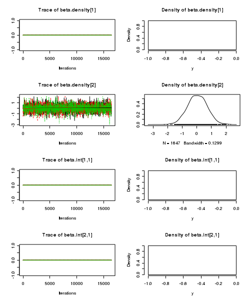
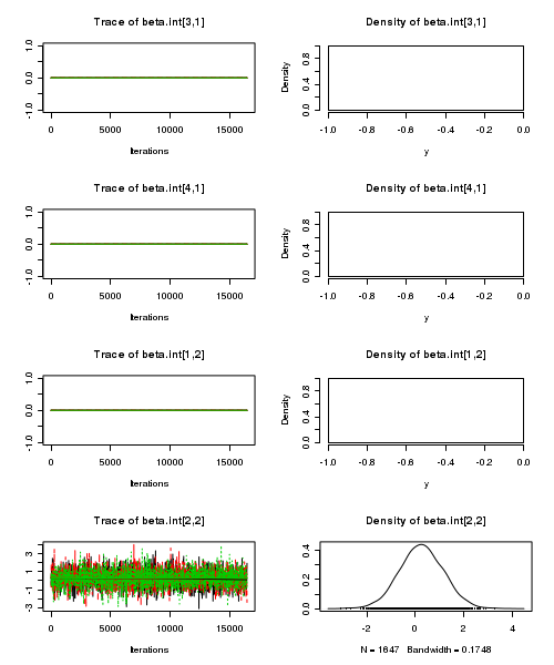
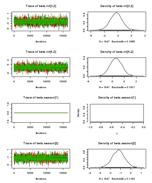
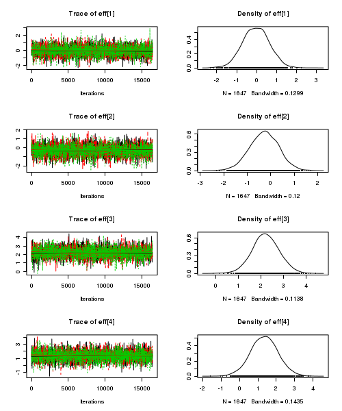
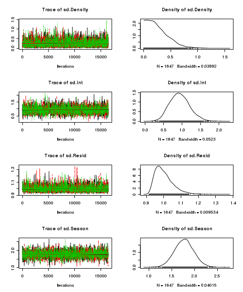
> plot(as.mcmc(quinn.r2jags))

- Raftery diagnostic
View code
> raftery.diag(as.mcmc(quinn.r2jags))
[[1]]

Quantile (q) = 0.025
Accuracy (r) = +/- 0.005
Probability (s) = 0.95

You need a sample size of at least 3746 with these values of q, r and s

[[2]]

Quantile (q) = 0.025
Accuracy (r) = +/- 0.005
Probability (s) = 0.95

You need a sample size of at least 3746 with these values of q, r and s

[[3]]

Quantile (q) = 0.025
Accuracy (r) = +/- 0.005
Probability (s) = 0.95

You need a sample size of at least 3746 with these values of q, r and s
- Autocorrelation
View code
> autocorr.diag(as.mcmc(quinn.r2jags))
         Mean[1,1] Mean[2,1] Mean[3,1]  Mean[4,1] Mean[1,2] Mean[2,2]  Mean[3,2] Mean[4,2]
Lag 0    1.0000000  1.000000  1.000000  1.0000000  1.000000  1.000000  1.000e+00  1.000000
Lag 10  -0.0082297  0.004866 -0.014512  0.0004189  0.019037  0.013411  4.773e-03 -0.008294
Lag 50   0.0008819 -0.003041 -0.005565  0.0035012  0.007405  0.013454 -1.337e-06  0.016589
Lag 100 -0.0060674 -0.009696 -0.006897 -0.0111460 -0.001689  0.014131 -2.677e-03  0.013051
Lag 500 -0.0119590 -0.001043 -0.019341  0.0072319 -0.008894 -0.009759 -2.027e-02  0.002028
        beta.density[1] beta.density[2] beta.int[1,1] beta.int[2,1] beta.int[3,1] beta.int[4,1]
Lag 0               NaN        1.000000           NaN           NaN           NaN           NaN
Lag 10              NaN        0.003179           NaN           NaN           NaN           NaN
Lag 50              NaN        0.007616           NaN           NaN           NaN           NaN
Lag 100             NaN       -0.010429           NaN           NaN           NaN           NaN
Lag 500             NaN       -0.011344           NaN           NaN           NaN           NaN
        beta.int[1,2] beta.int[2,2] beta.int[3,2] beta.int[4,2] beta.season[1] beta.season[2]
Lag 0             NaN     1.0000000      1.000000      1.000000            NaN       1.000000
Lag 10            NaN     0.0299663     -0.007553      0.005904            NaN      -0.011382
Lag 50            NaN     0.0000938      0.003024     -0.005636            NaN      -0.006023
Lag 100           NaN     0.0022546     -0.012278     -0.008113            NaN      -0.010964
Lag 500           NaN    -0.0093048     -0.002738     -0.025463            NaN      -0.010620
        beta.season[3] beta.season[4]      beta0  deviance    eff[1]    eff[2]    eff[3]    eff[4]
Lag 0          1.00000       1.000000  1.0000000  1.000000  1.000000  1.000000  1.000000  1.000000
Lag 10        -0.02272      -0.002790 -0.0082297 -0.004244  0.003179  0.028275 -0.001557 -0.009585
Lag 50         0.01592       0.004193  0.0008819  0.001471  0.007616 -0.004404 -0.015173  0.006090
Lag 100       -0.01495      -0.017531 -0.0060674  0.008789 -0.010429  0.015171 -0.019009 -0.009054
Lag 500       -0.01460      -0.019725 -0.0119590  0.008385 -0.011344 -0.007830 -0.026246 -0.003047
        sd.Density    sd.Int  sd.Resid  sd.Season sigma.res
Lag 0     1.000000  1.000000  1.000000  1.0000000  1.000000
Lag 10   -0.016133 -0.017361 -0.013893  0.0028862  0.008276
Lag 50    0.006714 -0.005050  0.017671 -0.0029169 -0.009613
Lag 100   0.019943  0.004759  0.008819 -0.0102643 -0.025626
Lag 500   0.014718 -0.025343  0.013722  0.0006947 -0.016266
- Trace plots
-
A summary figure would be nice
View code
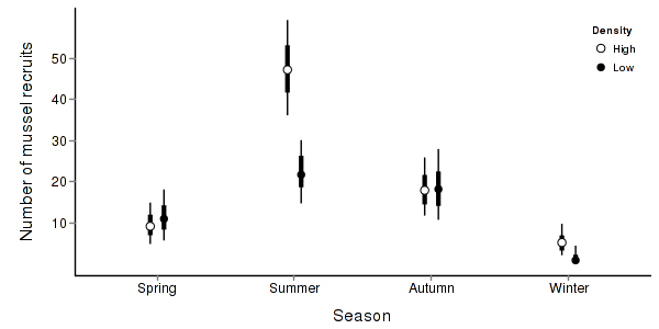
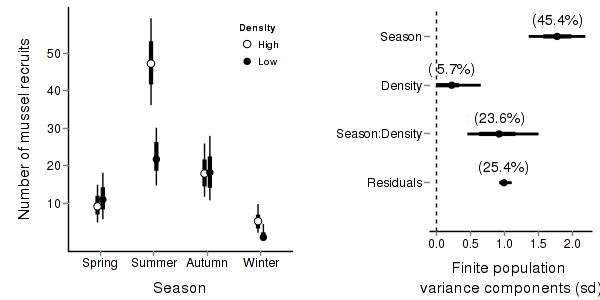
> quinn.mcmc <- as.mcmc(quinn.r2jags$BUGSoutput$sims.matrix)
> #get the column indexes for the parameters we are interested in
> quinn.sum <- summary.mcmc(quinn.mcmc, terms=c("Mean")) #or "alpha"
> quinn.sum <- cbind(quinn.sum, expand.grid(Season=c("Autumn","Spring","Summer","Winter"), Density=c("High","Low")))
>
> quinn.sum$Season <- factor(quinn.sum$Season, levels=c("Spring","Summer","Autumn","Winter"))
> library(scales)
>
> p1<-ggplot(quinn.sum,aes(y=mean, x=Season, group=Density))+
+ geom_errorbar(aes(ymin=lower, ymax=upper),width=0,size=1.5,position=position_dodge(0.2))+
+ geom_errorbar(aes(ymin=lower.1, ymax=upper.1),width=0,position=position_dodge(0.2))+
+ geom_point(aes(shape=Density, fill=Density),size=3,position=position_dodge(0.2))+
+ scale_y_continuous("Number of mussel recruits",
+   trans=trans_new("x2",function(x) x^2,"sqrt"),
+   breaks=sqrt(pretty(c(0,60))),
+   labels=pretty(c(0,60)))+
+ scale_x_discrete("Season")+
+ scale_shape_manual(name="Density",values=c(21,16), breaks=c("High","Low"), labels=c("High","Low"))+
+ scale_fill_manual(name="Density",values=c("white","black"), breaks=c("High","Low"), labels=c("High","Low"))+
+ murray_opts+opts(legend.position=c(1,0.99),legend.justification=c(1,1))
> p1
>
+
+ #Finite-population standard deviations
> quinn.sd <- summary.mcmc(quinn.mcmc, terms=c("sd"))
> rownames(quinn.sd) <- c("Density","Season:Density","Residuals","Season")
> quinn.sd$name <- factor(c("Density","Season:Density","Residuals","Season"), levels=c("Residuals", "Season:Density", "Density","Season"))
>
> p2<-ggplot(quinn.sd,aes(y=name, x=median))+
+ geom_vline(xintercept=0,linetype="dashed")+
+ geom_hline(xintercept=0)+
+ scale_x_continuous("Finite population \nvariance components (sd)")+
+ geom_errorbarh(aes(xmin=lower.1, xmax=upper.1), height=0, size=1)+
+ geom_errorbarh(aes(xmin=lower, xmax=upper), height=0, size=1.5)+
+ geom_point(size=3)+
+ geom_text(aes(label=sprintf("(%4.1f%%)",Perc),vjust=-1))+
+ murray_opts+
+ opts(axis.line=theme_blank(),axis.title.y=theme_blank(),
+ axis.text.y=theme_text(size=12,hjust=1))
>
> grid.newpage()
> pushViewport(viewport(layout=grid.layout(1,2,5,5,respect=TRUE)))
> pushViewport(viewport(layout.pos.col=1, layout.pos.row=1))
> print(p1,newpage=FALSE)
> popViewport(1)
> pushViewport(viewport(layout.pos.col=2, layout.pos.row=1))
> print(p2,newpage=FALSE)
> popViewport(0)
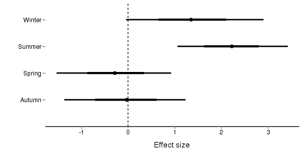
>
+
+ #eff
> quinn.eff <- summary.mcmc(quinn.mcmc, terms=c("eff\\["))
> nms <- c("Autumn","Spring","Summer","Winter")
> quinn.eff$name <- nms
>
> p3 <- ggplot(quinn.eff, aes(y=name, x=mean))+
+ geom_vline(xintercept=0,linetype="dashed")+
+ geom_hline(xintercept=0)+
+ geom_errorbarh(aes(xmin=lower.1, xmax=upper.1), height=0, size=1)+
+ geom_errorbarh(aes(xmin=lower, xmax=upper), height=0, size=1.5)+
+ geom_point(size=3)+murray_opts+
+ scale_x_continuous(name="Effect size")+
+ opts(axis.line=theme_blank(),axis.title.y=theme_blank(),
+ axis.text.y=theme_text(size=12,hjust=1))
> p3
>
+
+
+ #cohen's D
> #eff<-NULL
> #eff.sd <- NULL
> #for (i in seq(1,7,b=2)) {
> #  eff <-cbind(eff,quinn.mcmc[,i] - quinn.mcmc[,i+1])
> #  eff.sd <- cbind(eff.sd,mean(apply(quinn.mcmc[,i:(i+1)],2,sd)))
> #}
> #cohen <- sweep(eff,2,eff.sd,"/")
> #adply(cohen,2,function(x) {
> #   data.frame(mean=mean(x), median=median(x),
> #		 HPDinterval(as.mcmc(x), p=0.68), HPDinterval(as.mcmc(x)))
> #})