Workshop 9.5b - Analysis of Covariance (Bayesian)
23 April 2011
ANCOVA references
- McCarthy (2007) - Chpt 6
- Kery (2010) - Chpt 10
- Gelman & Hill (2007) - Chpt 4
- Logan (2010) - Chpt 12
- Quinn & Keough (2002) - Chpt 9
> library(R2jags)
> library(ggplot2)
> library(grid)
> #define my common ggplot options
> murray_opts <- opts(panel.grid.major=theme_blank(),
+ 			   panel.grid.minor=theme_blank(),
+ 			   panel.border = theme_blank(),
+ 			   panel.background = theme_blank(),
+ 			   axis.title.y=theme_text(size=15, vjust=0,angle=90),
+ 			   axis.text.y=theme_text(size=12),
+ 			   axis.title.x=theme_text(size=15, vjust=-1),
+ 			   axis.text.x=theme_text(size=12),
+ 			   axis.line = theme_segment(),
+ 			   legend.position=c(1,0.1),legend.justification=c(1,0),
+ 			   legend.key=theme_blank(),
+ 			   plot.margin=unit(c(0.5,0.5,1,2),"lines")
+ )
>
> #create a convenience function for predicting from mcmc objects
> predict.mcmc <- function(mcmc, terms=NULL, mmat, trans="identity") {
+   library(plyr)
+   library(coda)
+   if(is.null(terms)) mcmc.coefs <- mcmc
+   else 	{
+      iCol<-match(terms, colnames(mcmc))
+ 	 mcmc.coefs <- mcmc[,iCol]
+   }
+   t2=")"
+   if (trans=="identity") {
+ 	t1 <- ""
+ 	t2=""
+   }else if (trans=="log") {
+ 	t1="exp("
+   }else if (trans=="log10") {
+ 	t1="10^("
+   }else if (trans=="sqrt") {
+ 	t1="("
+ 	t2=")^2"
+   }
+   eval(parse(text=paste("mcmc.sum <-adply(mcmc.coefs %*% t(mmat),2,function(x) {
+ 	data.frame(mean=",t1,"mean(x)",t2,",
+     median=",t1,"median(x)",t2,",
+ 	",t1,"coda:::HPDinterval(as.mcmc(x), p=0.68)",t2,",
+ 	",t1,"coda:::HPDinterval(as.mcmc(x))",t2,"
+     )})", sep="")))
+
+   mcmc.sum
+ }
>
>
> #create a convenience function for summarizing mcmc objects
> summary.mcmc <- function(mcmc, terms=NULL, trans="identity") {
+   library(plyr)
+   library(coda)
+   if(is.null(terms)) mcmc.coefs <- mcmc
+   else 	{
+      iCol<-grep(terms, colnames(mcmc))
+ 	 mcmc.coefs <- mcmc[,iCol]
+   }
+   t2=")"
+   if (trans=="identity") {
+ 	t1 <- ""
+ 	t2=""
+   }else if (trans=="log") {
+ 	t1="exp("
+   }else if (trans=="log10") {
+ 	t1="10^("
+   }else if (trans=="sqrt") {
+ 	t1="("
+ 	t2=")^2"
+   }
+   eval(parse(text=paste("mcmc.sum <-adply(mcmc.coefs,2,function(x) {
+ 	data.frame(mean=",t1,"mean(x)",t2,",
+     median=",t1,"median(x)",t2,",
+ 	",t1,"coda:::HPDinterval(as.mcmc(x), p=0.68)",t2,",
+ 	",t1,"coda:::HPDinterval(as.mcmc(x))",t2,"
+     )})", sep="")))
+
+   mcmc.sum$Perc <-100*mcmc.sum$median/sum(mcmc.sum$median)
+   mcmc.sum
+ }
>
>
> theme_complete_bw <- function(base_size = 12) {
+   structure(list(
+     axis.line =         theme_blank(),
+     axis.text.x =       theme_text(size = base_size * 0.8 , lineheight = 0.9, colour = "black", vjust = 1),
+     axis.text.y =       theme_text(size = base_size * 0.8, lineheight = 0.9, colour = "black", hjust = 1),
+     axis.ticks =        theme_segment(colour = "black"),
+     axis.title.x =      theme_text(size = base_size, vjust = 0.5),
+     axis.title.y =      theme_text(size = base_size, angle = 90, vjust = 0.5),
+     axis.ticks.length = unit(0.15, "cm"),
+     axis.ticks.margin = unit(0.1, "cm"),
+
+     legend.background = theme_rect(colour=NA),
+     legend.key =        theme_rect(fill = NA, colour = "black", size = 0.25),
+     legend.key.size =   unit(1.2, "lines"),
+     legend.text =       theme_text(size = base_size * 0.8),
+     legend.title =      theme_text(size = base_size * 0.8, face = "bold", hjust = 0),
+     legend.position =   "right",
+
+     panel.background =  theme_rect(fill = NA, colour = "black", size = 0.25),
+     panel.border =      theme_blank(),
+     panel.grid.major =  theme_line(colour = "black", size = 0.05),
+     panel.grid.minor =  theme_line(colour = "black", size = 0.05),
+     panel.margin =      unit(0.25, "lines"),
+
+     strip.background =  theme_rect(fill = NA, colour = NA),
+     strip.text.x =      theme_text(colour = "black", size = base_size * 0.8),
+     strip.text.y =      theme_text(colour = "black", size = base_size * 0.8, angle = -90),
+
+     plot.background =   theme_rect(colour = NA, fill = "white"),
+     plot.title =        theme_text(size = base_size * 1.2),
+     plot.margin =       unit(c(1, 1, 0.5, 0.5), "lines")
+   ), class = "options")
+ }
Homogeneous slopes
To investigate the impacts of sexual activity on the fruitfly longevity, Partridge and Farquhar (1981), measured the longevity of male fruitflies with access to either one virgin female (potential mate), eight virgin females, one pregnant female (not a potential mate), eight pregnant females or no females. The pool of available male fruitflies varied in size and since size is known to impact longevity, the researchers also measured thorax length as a covariate.
Download Partridge1 data set| Format of partridge1.csv data file | ||||||||||||||||||||||
|---|---|---|---|---|---|---|---|---|---|---|---|---|---|---|---|---|---|---|---|---|---|---|
|
 |
Open the partridge1 data file. HINT.
> partridge <- read.table("../downloads/data/partridge1.csv",
+     header = T, sep = ",", strip.white = T)
> head(partridge)
  TREATMENT THORAX LONGEV
1     Preg8   0.64     35
2     Preg8   0.68     37
3     Preg8   0.68     49
4     Preg8   0.72     46
5     Preg8   0.72     63
6     Preg8   0.76     39
Exploratory data analysis suggested that log10 transformation of Longevity could normalize the data and improve linearity
-
Fit the appropriate multiplicative JAGS (BUGS) model ensuring that the predictors are centered (this can either be done in JAGS or in the data passed to JAGS).
- Additive model - assuming homogeneous slopes
Show code
> runif(1)[1] 0.9757
> modelString="
+ model {
+    #Likelihood
+    for (i in 1:n) {
+       loglongevity[i]~dnorm(mu[i],tau)
+       mu[i] <- alpha +beta.treatment[treatment[i]] + beta.thorax*cthorax[i]
+ 	  y.err[i] <- loglongevity[i] - mu[i]
+    }
+
+    #Priors
+    alpha ~ dnorm(0,1.0E-6)
+    beta.treatment[1] <- 0
+    for (i in 2:nTreatment) {
+      beta.treatment[i] ~ dnorm(0,1.0E-6)
+    }
+    beta.thorax ~ dnorm(0,1.0E-6)
+
+    sigma ~ dunif(0,100)
+    tau <- pow(sigma,2)
+
+    #Finite population standard deviations
+    sd.Treatment <- sd(beta.treatment)
+    sd.Thorax <- abs(beta.thorax)*sd(cthorax)
+    sd.Residuals <- sd(y.err)
+
+    #Treatment means (at middle of thorax size range)
+    for (i in 1:nTreatment) {
+      Treatment.means[i] <- alpha + beta.treatment[i]
+    }
+ }
+ "
> ## write the model to a text file (I suggest you alter the path to somewhere more relevant
> ## to your system!)
> writeLines(modelString,con="../downloads/BUGSscripts/ws9.5bQ1.1.txt")
>
> treat <- factor(partridge$TREATMENT, levels=c(unique(as.character(partridge$TREATMENT))))
> #center the thorax values. They should NOT be centered separately within each level of treatment
> partridge$cThorax <- scale(partridge$THORAX,scale=FALSE)[,1]
> partridge.list <- with(partridge,
+                       list(loglongevity=log10(LONGEV),
+ 					  treatment=as.numeric(treat),
+ 					  cthorax=cThorax,
+ 					  n=nrow(partridge), nTreatment=length(levels(TREATMENT))
+ ))
>
> #nominate the nodes to monitor (parameters)
> params <- c("alpha", "beta.treatment", "beta.thorax", "sigma",
+   "sd.Treatment","sd.Thorax", "sd.Residuals",
+    "Treatment.means"
+ )
> adaptSteps = 1000
> burnInSteps = 2000
> nChains = 3
> numSavedSteps = 5000
> thinSteps = 10
> nIter = ceiling((numSavedSteps * thinSteps)/nChains)
>
> partridge.r2jags <- jags(data=partridge.list,
+ 	  inits=NULL, #or inits=list(inits,inits,inits) # since there are three chains
+ 	  parameters.to.save=params,
+ 	  model.file="../downloads/BUGSscripts/ws9.5bQ1.1.txt",
+ 	  n.chains=3,
+ 	  n.iter=nIter,
+ 	  n.burnin=burnInSteps,
+       n.thin=10
+ 	  )
Compiling model graph Resolving undeclared variables Allocating nodes Graph Size: 578 Initializing model
> print(partridge.r2jags)Inference for Bugs model at "../downloads/BUGSscripts/ws9.5bQ1.1.txt", fit using jags, 3 chains, each with 16667 iterations (first 2000 discarded), n.thin = 10 n.sims = 4401 iterations saved mu.vect sd.vect 2.5% 25% 50% 75% 97.5% Rhat n.eff Treatment.means[1] 1.807 0.017 1.774 1.797 1.808 1.819 1.839 1.001 4400 Treatment.means[2] 1.771 0.017 1.738 1.759 1.771 1.782 1.804 1.001 4400 Treatment.means[3] 1.794 0.017 1.760 1.782 1.794 1.805 1.826 1.001 3200 Treatment.means[4] 1.717 0.017 1.684 1.706 1.717 1.729 1.749 1.001 2500 Treatment.means[5] 1.590 0.017 1.557 1.579 1.590 1.601 1.622 1.001 3600 alpha 1.807 0.017 1.774 1.797 1.808 1.819 1.839 1.001 4400 beta.thorax 1.194 0.099 1.001 1.126 1.195 1.260 1.390 1.002 2200 beta.treatment[1] 0.000 0.000 0.000 0.000 0.000 0.000 0.000 1.000 1 beta.treatment[2] -0.037 0.024 -0.084 -0.053 -0.037 -0.021 0.010 1.001 4400 beta.treatment[3] -0.014 0.024 -0.059 -0.029 -0.014 0.002 0.033 1.001 4400 beta.treatment[4] -0.090 0.024 -0.136 -0.107 -0.091 -0.074 -0.044 1.001 4400 beta.treatment[5] -0.218 0.023 -0.264 -0.234 -0.218 -0.202 -0.172 1.001 4400 sd.Residuals 0.083 0.001 0.082 0.083 0.083 0.084 0.086 1.002 1500 sd.Thorax 0.092 0.008 0.077 0.087 0.092 0.097 0.107 1.002 2200 sd.Treatment 0.080 0.007 0.066 0.075 0.080 0.085 0.095 1.001 4400 sigma 11.993 0.763 10.506 11.489 11.995 12.510 13.497 1.001 4400 deviance -264.624 3.791 -269.967 -267.435 -265.292 -262.652 -255.529 1.001 2800 For each parameter, n.eff is a crude measure of effective sample size, and Rhat is the potential scale reduction factor (at convergence, Rhat=1). DIC info (using the rule, pD = var(deviance)/2) pD = 7.2 and DIC = -257.4 DIC is an estimate of expected predictive error (lower deviance is better). - Multiplicative model - Heterogeneous slopes
Show code
> runif(1)[1] 0.1938
> modelString="
+ model {
+    #Likelihood
+    for (i in 1:n) {
+       loglongevity[i]~dnorm(mu[i],tau)
+       mu[i] <- alpha + beta.treatment[treatment[i]] + beta.thorax*cthorax[i] + beta.int[treatment[i]]*cthorax[i]
+ 	  y.err[i] <- loglongevity[i] - mu[i]
+    }
+
+    #Priors
+    alpha ~ dnorm(0,1.0E-6)
+    beta.treatment[1] <- 0
+    beta.int[1] <- 0
+    for (i in 2:nTreatment) {
+      beta.treatment[i] ~ dnorm(0,1.0E-6)
+      beta.int[i] ~ dnorm(0,1.0E-6)
+      #beta.treatment[i] ~ dnorm(mu.treatment,tau.treatment)
+      #beta.int[i] ~ dnorm(mu.int,tau.int)
+    }
+    beta.thorax ~ dnorm(0,1.0E-6)
+    #beta.thorax ~ dnorm(mu.thorax,tau.thorax)
+
+    sigma ~ dunif(0,100)
+    tau <- pow(sigma,2)
+
+    #Finite population standard deviations
+    sd.Treatment <- sd(beta.treatment)
+    sd.Thorax <- abs(beta.thorax)*sd(cthorax)
+    sd.Int <- sd(beta.int)*sd(cthorax)
+    sd.Residuals <- sd(y.err)
+
+    #Treatment means (at middle of thorax size range)
+    for (i in 1:nTreatment) {
+      Treatment.means[i] <- alpha + beta.treatment[i]
+    }
+ }
+ "
> ## write the model to a text file (I suggest you alter the path to somewhere more relevant
> ## to your system!)
> writeLines(modelString,con="../downloads/BUGSscripts/ws9.5bQ1.1b.txt")
>
> treat <- factor(partridge$TREATMENT, levels=c(unique(as.character(partridge$TREATMENT))))
> #center the thorax values. They should NOT be centered separately within each level of treatment
> partridge$cThorax <- scale(partridge$THORAX,scale=FALSE)[,1]
> partridge.list <- with(partridge,
+                       list(loglongevity=log10(LONGEV),
+ 					  treatment=as.numeric(treat),
+ 					  cthorax=cThorax,
+ 					  n=nrow(partridge), nTreatment=length(levels(TREATMENT))
+ ))
>
> #nominate the nodes to monitor (parameters)
> params <- c("alpha", "beta.treatment", "beta.thorax", "beta.int",
+    "sigma",
+   "sd.Treatment","sd.Thorax", "sd.Residuals","sd.Int",
+    "Treatment.means"#, "sigma.treatment","sigma.int","sigma.thorax"
+ )
> adaptSteps = 1000
> burnInSteps = 2000
> nChains = 3
> numSavedSteps = 5000
> thinSteps = 10
> nIter = ceiling((numSavedSteps * thinSteps)/nChains)
>
> partridge.r2jags2 <- jags(data=partridge.list,
+ 	  inits=NULL, #or inits=list(inits,inits,inits) # since there are three chains
+ 	  parameters.to.save=params,
+ 	  model.file="../downloads/BUGSscripts/ws9.5bQ1.1b.txt",
+ 	  n.chains=3,
+ 	  n.iter=nIter,
+ 	  n.burnin=burnInSteps,
+       n.thin=10
+ 	  )
Compiling model graph Resolving undeclared variables Allocating nodes Graph Size: 634 Initializing model
> print(partridge.r2jags2)Inference for Bugs model at "../downloads/BUGSscripts/ws9.5bQ1.1b.txt", fit using jags, 3 chains, each with 16667 iterations (first 2000 discarded), n.thin = 10 n.sims = 4401 iterations saved mu.vect sd.vect 2.5% 25% 50% 75% 97.5% Rhat n.eff Treatment.means[1] 1.806 0.017 1.773 1.795 1.806 1.818 1.839 1.001 4400 Treatment.means[2] 1.773 0.017 1.739 1.762 1.773 1.784 1.806 1.001 4400 Treatment.means[3] 1.795 0.017 1.762 1.783 1.795 1.806 1.827 1.002 2100 Treatment.means[4] 1.716 0.017 1.682 1.704 1.716 1.728 1.751 1.001 3700 Treatment.means[5] 1.598 0.017 1.565 1.587 1.598 1.610 1.632 1.001 4400 alpha 1.806 0.017 1.773 1.795 1.806 1.818 1.839 1.001 4400 beta.int[1] 0.000 0.000 0.000 0.000 0.000 0.000 0.000 1.000 1 beta.int[2] -0.096 0.287 -0.664 -0.291 -0.098 0.096 0.475 1.001 4400 beta.int[3] -0.194 0.322 -0.822 -0.407 -0.200 0.022 0.431 1.001 4400 beta.int[4] 0.136 0.320 -0.486 -0.075 0.131 0.343 0.776 1.001 4400 beta.int[5] 0.514 0.302 -0.049 0.313 0.508 0.719 1.109 1.001 4400 beta.thorax 1.123 0.206 0.718 0.989 1.124 1.263 1.521 1.001 4400 beta.treatment[1] 0.000 0.000 0.000 0.000 0.000 0.000 0.000 1.000 1 beta.treatment[2] -0.033 0.024 -0.079 -0.049 -0.033 -0.017 0.014 1.001 4400 beta.treatment[3] -0.011 0.024 -0.059 -0.027 -0.011 0.005 0.035 1.001 3900 beta.treatment[4] -0.090 0.024 -0.137 -0.106 -0.090 -0.074 -0.044 1.001 3500 beta.treatment[5] -0.208 0.024 -0.256 -0.224 -0.207 -0.192 -0.161 1.001 4400 sd.Int 0.024 0.007 0.010 0.019 0.024 0.028 0.037 1.001 4400 sd.Residuals 0.083 0.001 0.080 0.081 0.082 0.083 0.086 1.001 4400 sd.Thorax 0.087 0.016 0.055 0.076 0.087 0.097 0.117 1.001 4400 sd.Treatment 0.077 0.008 0.063 0.072 0.077 0.082 0.092 1.001 4400 sigma 12.093 0.798 10.631 11.548 12.077 12.626 13.691 1.001 4400 deviance -266.895 4.935 -274.556 -270.560 -267.548 -264.019 -255.495 1.001 4400 For each parameter, n.eff is a crude measure of effective sample size, and Rhat is the potential scale reduction factor (at convergence, Rhat=1). DIC info (using the rule, pD = var(deviance)/2) pD = 12.2 and DIC = -254.7 DIC is an estimate of expected predictive error (lower deviance is better).
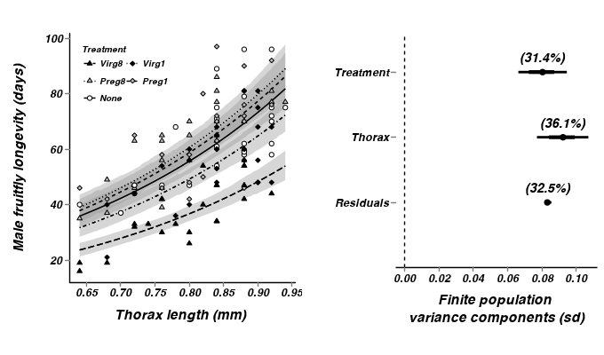
- Additive model - assuming homogeneous slopes
- Generate a summary figure
- From the additive model - homogeneous slopes
Show code
> library(scales)
> #get the effects mcmc matrix
> partridge.mcmc <- as.mcmc(partridge.r2jags$BUGSoutput$sims.matrix)[,c("alpha","beta.treatment[2]", "beta.treatment[3]", "beta.treatment[4]", "beta.treatment[5]","beta.thorax")]
> # develop an appropriate model matrix
> xx <- with(partridge, seq(min(cThorax), max(cThorax), l=100))
>
> newdata <- expand.grid(cThorax=xx, TREATMENT=unique(as.character(partridge$TREATMENT)))
> partridge.mmat <- model.matrix(~TREATMENT+cThorax, data=newdata)
> pred <- predict.mcmc(mcmc=partridge.mcmc, mmat=partridge.mmat)
> partridge.pred <- cbind(newdata,pred)
>
> partridge$TREATMENT <-factor(partridge$TREATMENT, levels=c("None","Preg1","Preg8","Virg1","Virg8"))
> partridge.pred$TREATMENT <-factor(partridge.pred$TREATMENT, levels=c("None","Preg1","Preg8","Virg1","Virg8"))
> thorax.mean <- mean(partridge$THORAX)
> p1 <- ggplot(data=partridge, aes(x=cThorax, y=log10(LONGEV), group=TREATMENT)) +
+   geom_smooth(data=partridge.pred, aes(y=mean, ymin=lower.1, ymax=upper.1, x=cThorax, linetype=TREATMENT),colour="black",stat="identity", show_guide=FALSE)+
+   geom_smooth(data=partridge.pred, aes(y=mean, x=cThorax,linetype=TREATMENT),colour="black",stat="identity", se=FALSE)+
+   geom_point(aes(shape=TREATMENT, fill=TREATMENT))+
+   scale_y_continuous(expression(paste("Male fruitfly longevity (days)", sep="")),
+      #trans=log_trans())+
+     trans=trans_new("power", function(x) 10^x, function(x) log10(x)),
+ 	breaks=trans_breaks(function(x) 10^x, "log10"),
+ 	labels=trans_format(function(x) 10^x, "log10"))+
+   scale_x_continuous(expression(paste("Thorax length (mm)", "\n", sep="")),
+ 	trans=trans_new("center", transform=function(x) {x+thorax.mean}, inverse=function(x) {x-thorax.mean}),
+ 	breaks=trans_breaks(function(x) {x+thorax.mean}, function(x) {x-thorax.mean}),
+ 	labels=trans_format(function(x) {x+thorax.mean},format=format_format()))+
+   scale_linetype_manual(name="Treatment", breaks=c("None","Preg1","Preg8","Virg1","Virg8"), values=c(1,2,3,4,5))+
+   scale_fill_manual(name="Treatment", breaks=c("None","Preg1","Preg8","Virg1","Virg8"), values=c("white","grey","grey","black","black"))+
+   scale_shape_manual(name="Treatment", breaks=c("None","Preg1","Preg8","Virg1","Virg8"), values=c(21,23,24,23,24))+
+   murray_opts+opts(legend.position=c(0,1),legend.justification=c(0,1))+
+ 	  guides(shape=guide_legend(ncol=2,byrow=TRUE, reverse=TRUE),fill=guide_legend(ncol=2,byrow=TRUE, reverse=TRUE), linetype=guide_legend(ncol=2,byrow=TRUE,reverse=TRUE))
>
> #Finite-population standard deviations
> partridge.sd <- summary.mcmc(as.mcmc(partridge.r2jags$BUGSoutput$sims.matrix), terms=c("sd"))
> rownames(partridge.sd) <- c("Residuals", "Thorax", "Treatment")
> partridge.sd$name <- factor(c("Residuals", "Thorax", "Treatment"), levels=c("Residuals", "Thorax", "Treatment"))
> p2<-ggplot(partridge.sd,aes(y=name, x=median))+
+   geom_vline(xintercept=0,linetype="dashed")+
+   geom_hline(xintercept=0)+
+   scale_x_continuous("Finite population \nvariance components (sd)")+
+   geom_errorbarh(aes(xmin=lower.1, xmax=upper.1), height=0, size=1)+
+   geom_errorbarh(aes(xmin=lower, xmax=upper), height=0, size=1.5)+
+   geom_point(size=3)+
+   geom_text(aes(label=sprintf("(%4.1f%%)",Perc),vjust=-1))+
+   murray_opts+
+   opts(axis.line=theme_blank(),axis.title.y=theme_blank(),
+   axis.text.y=theme_text(size=12,hjust=1))
>
> grid.newpage()
> pushViewport(viewport(layout=grid.layout(1,2,5,5,respect=TRUE)))
> pushViewport(viewport(layout.pos.col=1, layout.pos.row=1))
> print(p1,newpage=FALSE)
> popViewport(1)
> pushViewport(viewport(layout.pos.col=2, layout.pos.row=1))
> print(p2,newpage=FALSE)
> popViewport(0)
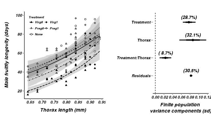
- From the multiplicative model - heterogeneous slopes
Show code
> library(scales)
> #get the effects mcmc matrix
> partridge.mcmc2 <- as.mcmc(partridge.r2jags2$BUGSoutput$sims.matrix)
> partridge.mcmc2 <- partridge.mcmc2[,c("alpha","beta.treatment[2]", "beta.treatment[3]", "beta.treatment[4]", "beta.treatment[5]","beta.thorax",
+                                 "beta.int[2]","beta.int[3]","beta.int[4]","beta.int[5]")]
>
>
>
> # develop an appropriate model matrix
> xx <- with(partridge, seq(min(cThorax), max(cThorax), l=100))
>
> newdata <- expand.grid(cThorax=xx, TREATMENT=unique(as.character(partridge$TREATMENT)))
> partridge.mmat2 <- model.matrix(~TREATMENT*cThorax, data=newdata)
> pred <- predict.mcmc(mcmc=partridge.mcmc2, mmat=partridge.mmat2)
> partridge.pred2 <- cbind(newdata,pred)
>
> partridge$TREATMENT <-factor(partridge$TREATMENT, levels=c("None","Preg1","Preg8","Virg1","Virg8"))
> partridge.pred2$TREATMENT <-factor(partridge.pred2$TREATMENT, levels=c("None","Preg1","Preg8","Virg1","Virg8"))
> thorax.mean <- mean(partridge$THORAX)
> p1 <- ggplot(data=partridge, aes(x=cThorax, y=log10(LONGEV), group=TREATMENT)) +
+   geom_smooth(data=partridge.pred2, aes(y=mean, ymin=lower.1, ymax=upper.1, x=cThorax, linetype=TREATMENT),colour="black",stat="identity", show_guide=FALSE)+
+   geom_smooth(data=partridge.pred2, aes(y=mean, x=cThorax,linetype=TREATMENT),colour="black",stat="identity", se=FALSE)+
+   geom_point(aes(shape=TREATMENT, fill=TREATMENT))+
+   scale_y_continuous(expression(paste("Male fruitfly longevity (days)", sep="")),
+      #trans=log_trans())+
+     trans=trans_new("power", function(x) 10^x, function(x) log10(x)),
+ 	breaks=trans_breaks(function(x) 10^x, "log10"),
+ 	labels=trans_format(function(x) 10^x, "log10"))+
+   scale_x_continuous(expression(paste("Thorax length (mm)", "\n", sep="")),
+ 	trans=trans_new("center", transform=function(x) {x+thorax.mean}, inverse=function(x) {x-thorax.mean}),
+ 	breaks=trans_breaks(function(x) {x+thorax.mean}, function(x) {x-thorax.mean}),
+ 	labels=trans_format(function(x) {x+thorax.mean},format=format_format()))+
+   scale_linetype_manual(name="Treatment", breaks=c("None","Preg1","Preg8","Virg1","Virg8"), values=c(1,2,3,4,5))+
+   scale_fill_manual(name="Treatment", breaks=c("None","Preg1","Preg8","Virg1","Virg8"), values=c("white","grey","grey","black","black"))+
+   scale_shape_manual(name="Treatment", breaks=c("None","Preg1","Preg8","Virg1","Virg8"), values=c(21,23,24,23,24))+
+   murray_opts+opts(legend.position=c(0,1),legend.justification=c(0,1))+
+ 	  guides(shape=guide_legend(ncol=2,byrow=TRUE, reverse=TRUE),fill=guide_legend(ncol=2,byrow=TRUE, reverse=TRUE), linetype=guide_legend(ncol=2,byrow=TRUE,reverse=TRUE))
>
>
> #Finite-population standard deviations
> partridge.sd2 <- summary.mcmc(as.mcmc(partridge.r2jags2$BUGSoutput$sims.matrix), terms=c("sd"))
> rownames(partridge.sd2) <- c("Treatment:Thorax","Residuals", "Thorax", "Treatment")
> partridge.sd2$name <- factor(c("Treatment:Thorax","Residuals","Thorax", "Treatment"), levels=c("Residuals", "Treatment:Thorax","Thorax", "Treatment"))
> p2<-ggplot(partridge.sd2,aes(y=name, x=median))+
+   geom_vline(xintercept=0,linetype="dashed")+
+   geom_hline(xintercept=0)+
+   scale_x_continuous("Finite population \nvariance components (sd)")+
+   geom_errorbarh(aes(xmin=lower.1, xmax=upper.1), height=0, size=1)+
+   geom_errorbarh(aes(xmin=lower, xmax=upper), height=0, size=1.5)+
+   geom_point(size=3)+
+   geom_text(aes(label=sprintf("(%4.1f%%)",Perc),vjust=-1))+
+   murray_opts+
+   opts(axis.line=theme_blank(),axis.title.y=theme_blank(),
+   axis.text.y=theme_text(size=12,hjust=1))
>
> grid.newpage()
> pushViewport(viewport(layout=grid.layout(1,2,widths=5,5,respect=TRUE)))
> pushViewport(viewport(layout.pos.col=1, layout.pos.row=1))
> print(p1,newpage=FALSE)
> popViewport(1)
> pushViewport(viewport(layout.pos.col=2, layout.pos.row=1))
> print(p2,newpage=FALSE)
> popViewport(0)
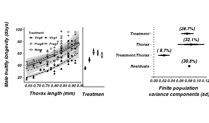
 Show code
> partridge.sum <- summary.mcmc(as.mcmc(partridge.r2jags2$BUGSoutput$sims.matrix), terms=c("Treatment.means"))
> partridge.sum$TREATMENT <- factor(unique(as.character(partridge$TREATMENT)),levels=c("Virg8","Virg1","Preg8","Preg1","None"))
> p0 <- ggplot(data=partridge, aes(y=log10(LONGEV), x=TREATMENT))+
+    geom_errorbar(data=partridge.sum,aes(y=mean,ymin=lower.1, ymax=upper.1), width=0, size=1)+
+    geom_errorbar(data=partridge.sum,aes(y=mean,ymin=lower, ymax=upper), width=0, size=1.5)+
+    geom_point(data=partridge.sum,aes(y=mean,shape=TREATMENT,fill=TREATMENT), size=2.5, show_guide=FALSE)+
+    geom_blank()+
+   scale_fill_manual(name="Treatment", breaks=c("None","Preg1","Preg8","Virg1","Virg8"), values=rev(c("white","grey","grey","black","black")))+
+   scale_shape_manual(name="Treatment", breaks=c("None","Preg1","Preg8","Virg1","Virg8"), values=rev(c(21,23,24,23,24)))+
+     scale_y_continuous(expression(paste("Male fruitfly longevity (days)", sep="")),
+      #trans=log_trans())+
+     trans=trans_new("power", function(x) 10^x, function(x) log10(x)),
+ 	breaks=trans_breaks(function(x) 10^x, "log10"),
+ 	labels=trans_format(function(x) 10^x, "log10"))+
+   scale_x_discrete("Treatment")+
+   murray_opts+
+   opts(plot.margin=unit(c(0.5,0,1,-1),"lines"),
+                    axis.text.y=theme_blank(), axis.title.y=theme_blank(),
+                    axis.text.x=theme_blank(),
+                    #axis.line=theme_blank(),
+                    axis.tick.length=unit(0,"cm"), axis.ticks.margin=unit(0,"cm"),
+                    axis.ticks=theme_blank()#,panel.margin=unit(0,"lines")
+                    )
>
>
> grid.newpage()
> pushViewport(viewport(layout=grid.layout(1,3,widths=c(8,2,10),7,respect=TRUE)))
> pushViewport(viewport(layout.pos.col=1, layout.pos.row=1))
> print(p1,newpage=FALSE)
> popViewport(1)
> pushViewport(viewport(layout.pos.col=2, layout.pos.row=1))
> print(p0,newpage=FALSE)
> popViewport(1)
> pushViewport(viewport(layout.pos.col=3, layout.pos.row=1))
> print(p2,newpage=FALSE)
> popViewport(0)
>
>
>
> #1. create the plot
> #2. use grid.ls() to get the list of grobs
> #3. edit or remove the grob
>
> #dt <- data.frame(y=rnorm(100), x=rnorm(100))
> #pp <- ggplot(dt,aes(y=y,x=x)) + geom_point()+
> #  opts(axis.line = theme_segment(colour = 'black', size = 2),
> #       panel.margin=unit(0,"null"),
> #       plot.margin=unit(rep(0,4),"null"),
> #       axis.ticks = theme_blank(),
> #    axis.text.x = theme_blank(),
> #    axis.text.y = theme_blank(),
> #    axis.title.x = theme_blank(),
> #    axis.title.y = theme_blank(),
> #    axis.ticks.length = unit(0,"null"),
> #    axis.ticks.margin = unit(0,"null"))
> #       #panel.margin=unit(c(0,0,-2,-2),"lines"))
> #pp
>
> ##grid.remove(gPath("axis-l", "axis.line.segments"), grep=TRUE)
> #grid.edit(gPath("axis-l", "axis.line.segments"), grep=TRUE, gp=gpar(col="blue"))
>
>
> #grid.edit(gPath("axis-l", "axis.line.segments"), grep=TRUE, gp=gpar(col="red"))
> #grid.edit(gPath("axis-b", "axis.line.segments"), grep=TRUE, gp=gpar(col="blue"))
>
>
> #library(gtable)
- From the additive model - homogeneous slopes
Heterogeneous slopes
Constable (1993) compared the inter-radial suture widths of urchins maintained on one of three food regimes (Initial: no additional food supplied above what was in the initial sample, low: food supplied periodically and high: food supplied ad libitum. In an attempt to control for substantial variability in urchin sizes, the initial body volume of each urchin was measured as a covariate.
Download Constable data set| Format of constable.csv data file | ||||||||||||||||||||||
|---|---|---|---|---|---|---|---|---|---|---|---|---|---|---|---|---|---|---|---|---|---|---|
|
 |
Open the constable data file. HINT.
> constable <- read.table("../downloads/data/constable.csv", header = T,
+     sep = ",", strip.white = T)
> head(constable)
    TREAT   IV  SUTW
1 Initial  3.5 0.010
2 Initial  5.0 0.020
3 Initial  8.0 0.061
4 Initial 10.0 0.051
5 Initial 13.0 0.041
6 Initial 13.0 0.061
Exploratory data analysis revealed some degree of non-linearity that could be improved by a cube-root transformation of the initial volume (IV) variable. A cube-root is achieved by raising a value to the power of one third (1/3).
-
Fit the appropriate multiplicative JAGS (BUGS) model ensuring that the predictors are centered (this can either be done in JAGS or in the data passed to JAGS).
-
Additive model - assuming homogeneous slopes. In an additive model, it is not necessary to center the covariate, as the slopes are assumed to be equal (lines parallel),
yet it is good practice all the same.
Show code
> runif(1)[1] 0.4364
> modelString="
+ model {
+    #Likelihood
+    for (i in 1:n) {
+       sutw[i]~dnorm(mu[i],tau)
+       mu[i] <- alpha +beta.treatment[treatment[i]] + beta.iv*cIv3[i]
+ 	  y.err[i] <- sutw[i] - mu[i]
+    }
+
+    #Priors
+    alpha ~ dnorm(0,1.0E-6)
+    beta.treatment[1] <- 0
+    for (i in 2:nTreatment) {
+      beta.treatment[i] ~ dnorm(0,1.0E-6)
+    }
+    beta.iv ~ dnorm(0,1.0E-6)
+
+    sigma ~ dunif(0,100)
+    tau <- pow(sigma,2)
+
+    #Finite population standard deviations
+    sd.Treatment <- sd(beta.treatment)
+    sd.IV <- abs(beta.iv)*sd(cIv3)
+    sd.Residuals <- sd(y.err)
+
+    #Treatment means (at middle of thorax size range)
+    for (i in 1:nTreatment) {
+      Treatment.means[i] <- alpha + beta.treatment[i]
+    }
+ }
+ "
> ## write the model to a text file (I suggest you alter the path to somewhere more relevant
> ## to your system!)
> writeLines(modelString,con="../downloads/BUGSscripts/ws9.5bQ2.1.txt")
>
> treat <- factor(constable$TREAT, levels=c(unique(as.character(constable$TREAT))))
> #center the cube-rott IV values. They should NOT be centered separately within each level of treatment
> constable$cIv3 <- scale(constable$IV^(1/3),scale=FALSE)[,1]
> constable.list <- with(constable,
+                       list(sutw=SUTW,
+ 					  treatment=as.numeric(treat),
+ 					  cIv3=cIv3,
+ 					  n=nrow(constable), nTreatment=length(levels(TREAT))
+ ))
>
> #nominate the nodes to monitor (parameters)
> params <- c("alpha", "beta.treatment", "beta.iv", "sigma",
+   "sd.Treatment","sd.IV", "sd.Residuals",
+    "Treatment.means"
+ )
> adaptSteps = 1000
> burnInSteps = 2000
> nChains = 3
> numSavedSteps = 5000
> thinSteps = 10
> nIter = ceiling((numSavedSteps * thinSteps)/nChains)
>
> constable.r2jags <- jags(data=constable.list,
+ 	  inits=NULL, #or inits=list(inits,inits,inits) # since there are three chains
+ 	  parameters.to.save=params,
+ 	  model.file="../downloads/BUGSscripts/ws9.5bQ2.1.txt",
+ 	  n.chains=3,
+ 	  n.iter=nIter,
+ 	  n.burnin=burnInSteps,
+       n.thin=10
+ 	  )
Compiling model graph Resolving undeclared variables Allocating nodes Graph Size: 411 Initializing model
> print(constable.r2jags)Inference for Bugs model at "../downloads/BUGSscripts/ws9.5bQ2.1.txt", fit using jags, 3 chains, each with 16667 iterations (first 2000 discarded), n.thin = 10 n.sims = 4401 iterations saved mu.vect sd.vect 2.5% 25% 50% 75% 97.5% Rhat n.eff Treatment.means[1] 0.066 0.005 0.057 0.063 0.066 0.069 0.075 1.001 3200 Treatment.means[2] 0.057 0.004 0.049 0.054 0.057 0.060 0.066 1.001 4400 Treatment.means[3] 0.094 0.004 0.085 0.091 0.094 0.097 0.103 1.001 4400 alpha 0.066 0.005 0.057 0.063 0.066 0.069 0.075 1.001 3200 beta.iv 0.025 0.005 0.015 0.022 0.026 0.029 0.036 1.003 4400 beta.treatment[1] 0.000 0.000 0.000 0.000 0.000 0.000 0.000 1.000 1 beta.treatment[2] -0.009 0.006 -0.021 -0.013 -0.009 -0.004 0.004 1.001 2600 beta.treatment[3] 0.028 0.006 0.015 0.024 0.028 0.032 0.040 1.002 2400 sd.IV 0.012 0.003 0.007 0.011 0.012 0.014 0.018 1.003 4400 sd.Residuals 0.021 0.000 0.021 0.021 0.021 0.022 0.022 1.001 4400 sd.Treatment 0.016 0.003 0.011 0.014 0.016 0.017 0.021 1.001 4400 sigma 46.669 3.926 39.134 43.974 46.675 49.234 54.663 1.001 4400 deviance -347.115 3.246 -351.432 -349.529 -347.742 -345.391 -339.153 1.001 4400 For each parameter, n.eff is a crude measure of effective sample size, and Rhat is the potential scale reduction factor (at convergence, Rhat=1). DIC info (using the rule, pD = var(deviance)/2) pD = 5.3 and DIC = -341.8 DIC is an estimate of expected predictive error (lower deviance is better). -
Multiplicative model - allowing heterogeneous slopes.
In an multiplicative model the slopes (lines) are not necessarily equal (parallel). Recall that the treatment effect in ANCOVA is measured as the difference in y-intercepts between the treatment levels. In a multiplicative model with heterogeneous slopes, the difference between treatments will depend on where along the covariate you are considering. Moreover, the differences in values when the covariate equals zero are unlikely to be of much biological interest. These values of the covariate are often outside the bounds of the data.
If we are interested in gaining an overall effect of treatment, then arguably, this should be the difference in treatments at the mean covariate value. Hence, it is best to center the covariate prior to analysis. Note, it is also probably more informative to explore the treatment effects at a range of covariate values.
Show code> runif(1)[1] 0.5745
> modelString="
+ model {
+    #Likelihood
+    for (i in 1:n) {
+       sutw[i]~dnorm(mu[i],tau)
+       mu[i] <- alpha +beta.treatment[treatment[i]] + beta.iv*cIv3[i] + beta.int[treatment[i]]*cIv3[i]
+ 	  y.err[i] <- sutw[i] - mu[i]
+    }
+
+    #Priors
+    alpha ~ dnorm(0,1.0E-6)
+    beta.treatment[1] <- 0
+    beta.int[1]<-0
+    for (i in 2:nTreatment) {
+      beta.treatment[i] ~ dnorm(0,1.0E-6)
+      beta.int[i] ~ dnorm(0,1.0E-6)
+    }
+    beta.iv ~ dnorm(0,1.0E-6)
+
+    sigma ~ dunif(0,100)
+    tau <- pow(sigma,2)
+
+
+    #Finite population standard deviations
+    sd.Treatment <- sd(beta.treatment)
+    sd.IV <- abs(beta.iv)*sd(cIv3)
+    sd.Int <- sd(beta.int)*sd(cIv3)
+    sd.Residuals <- sd(y.err)
+
+    #Treatment means (at middle of thorax size range)
+    for (i in 1:nTreatment) {
+      Treatment.means[i] <- alpha + beta.treatment[i]
+    }
+ }
+ "
> ## write the model to a text file (I suggest you alter the path to somewhere more relevant
> ## to your system!)
> writeLines(modelString,con="../downloads/BUGSscripts/ws9.5bQ2.1b.txt")
>
> treat <- factor(constable$TREAT, levels=c(unique(as.character(constable$TREAT))))
> #center the cube-rott IV values. They should NOT be centered separately within each level of treatment
> constable$cIv3 <- scale(constable$IV^(1/3),scale=FALSE)[,1]
> constable.list <- with(constable,
+                       list(sutw=SUTW,
+ 					  treatment=as.numeric(treat),
+ 					  cIv3=cIv3,
+ 					  n=nrow(constable), nTreatment=length(levels(TREAT))
+ ))
>
> #nominate the nodes to monitor (parameters)
> params <- c("alpha", "beta.treatment", "beta.int","beta.iv", "sigma",
+   "sd.Treatment","sd.IV", "sd.Int","sd.Residuals",
+    "Treatment.means"
+ )
> adaptSteps = 1000
> burnInSteps = 2000
> nChains = 3
> numSavedSteps = 5000
> thinSteps = 10
> nIter = ceiling((numSavedSteps * thinSteps)/nChains)
>
> constable.r2jags2 <- jags(data=constable.list,
+ 	  inits=NULL, #or inits=list(inits,inits,inits) # since there are three chains
+ 	  parameters.to.save=params,
+ 	  model.file="../downloads/BUGSscripts/ws9.5bQ2.1b.txt",
+ 	  n.chains=3,
+ 	  n.iter=nIter,
+ 	  n.burnin=burnInSteps,
+       n.thin=10
+ 	  )
Compiling model graph Resolving undeclared variables Allocating nodes Graph Size: 474 Initializing model
> print(constable.r2jags2)Inference for Bugs model at "../downloads/BUGSscripts/ws9.5bQ2.1b.txt", fit using jags, 3 chains, each with 16667 iterations (first 2000 discarded), n.thin = 10 n.sims = 4401 iterations saved mu.vect sd.vect 2.5% 25% 50% 75% 97.5% Rhat n.eff Treatment.means[1] 0.066 0.004 0.057 0.063 0.066 0.069 0.074 1.001 4400 Treatment.means[2] 0.059 0.004 0.051 0.056 0.059 0.062 0.068 1.001 4400 Treatment.means[3] 0.097 0.005 0.088 0.093 0.096 0.100 0.105 1.001 4400 alpha 0.066 0.004 0.057 0.063 0.066 0.069 0.074 1.001 4400 beta.int[1] 0.000 0.000 0.000 0.000 0.000 0.000 0.000 1.000 1 beta.int[2] -0.027 0.011 -0.049 -0.034 -0.026 -0.019 -0.005 1.001 4400 beta.int[3] 0.011 0.015 -0.018 0.001 0.011 0.021 0.041 1.001 4400 beta.iv 0.036 0.008 0.019 0.030 0.036 0.041 0.052 1.001 4400 beta.treatment[1] 0.000 0.000 0.000 0.000 0.000 0.000 0.000 1.000 1 beta.treatment[2] -0.007 0.006 -0.019 -0.011 -0.007 -0.003 0.005 1.001 4400 beta.treatment[3] 0.031 0.006 0.019 0.027 0.031 0.035 0.043 1.001 4400 sd.IV 0.017 0.004 0.009 0.015 0.018 0.020 0.025 1.001 4400 sd.Int 0.008 0.003 0.004 0.007 0.008 0.010 0.013 1.001 4400 sd.Residuals 0.020 0.000 0.020 0.020 0.020 0.021 0.022 1.002 1300 sd.Treatment 0.017 0.003 0.011 0.015 0.017 0.018 0.021 1.001 4400 sigma 49.080 4.291 41.138 46.095 49.042 51.862 57.482 1.002 1600 deviance -354.492 3.920 -359.980 -357.374 -355.178 -352.442 -345.030 1.002 2000 For each parameter, n.eff is a crude measure of effective sample size, and Rhat is the potential scale reduction factor (at convergence, Rhat=1). DIC info (using the rule, pD = var(deviance)/2) pD = 7.7 and DIC = -346.8 DIC is an estimate of expected predictive error (lower deviance is better).
-
Additive model - assuming homogeneous slopes. In an additive model, it is not necessary to center the covariate, as the slopes are assumed to be equal (lines parallel),
yet it is good practice all the same.
- Generate a summary figure
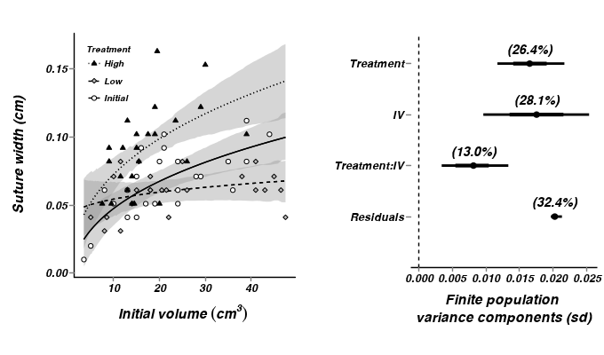
- From the multiplicative model - heterogeneous slopes
Show code
> library(scales)
> ## get the effects mcmc matrix
> constable.mcmc <- as.mcmc(constable.r2jags2$BUGSoutput$sims.matrix)[,
+     c("alpha", "beta.treatment[2]", "beta.treatment[3]", "beta.iv", "beta.int[2]",
+         "beta.int[3]")]
> ## develop an appropriate model matrix
> xx <- with(constable, seq(min(cIv3), max(cIv3), l = 100))
>
> newdata <- expand.grid(cIv3 = xx, TREAT = unique(as.character(constable$TREAT)))
> constable.mmat <- model.matrix(~TREAT * cIv3, data = newdata)
> pred <- predict.mcmc(mcmc = constable.mcmc, mmat = constable.mmat)
> constable.pred <- cbind(newdata, pred)
>
> xlevels <- unique(as.character(constable$TREAT))
> constable$TREAT <- factor(constable$TREAT, levels = xlevels)
> constable.pred$TREAT <- factor(constable.pred$TREAT, levels = xlevels)
> iv3.mean <- mean(constable$IV^(1/3))
> iv.mean <- iv3.mean^3
>
> p1 <- ggplot(data = constable, aes(x = cIv3, y = SUTW, group = TREAT)) +
+     geom_smooth(data = constable.pred, aes(y = mean, ymin = lower.1, ymax = upper.1,
+         x = cIv3, linetype = TREAT), colour = "black", stat = "identity", show_guide = FALSE) +
+     geom_smooth(data = constable.pred, aes(y = mean, x = cIv3, linetype = TREAT),
+         colour = "black", stat = "identity", se = FALSE) + geom_point(aes(shape = TREAT,
+     fill = TREAT)) + scale_y_continuous(expression(paste("Suture width (cm)",
+     sep = ""))) + scale_x_continuous(expression(paste("Initial volume ", (cm^3),
+     "\n", sep = "")), trans = trans_new("center", transform = function(x) {
+     x1 <- x + iv3.mean
+     x1^3
+ }, inverse = function(x) {
+     x1 <- x^(1/3)
+     x2 <- x1 - iv3.mean
+ }), breaks = trans_breaks(function(x) {
+     (x + iv3.mean)^3
+ }, function(x) {
+     (x^(1/3)) - iv3.mean
+ }), labels = trans_format(function(x) {
+     (x + iv3.mean)^3
+ }, format = format_format())) + scale_linetype_manual(name = "Treatment", breaks = xlevels,
+     values = c(1, 2, 3)) + scale_fill_manual(name = "Treatment", breaks = xlevels,
+     values = c("white", "grey", "black")) + scale_shape_manual(name = "Treatment",
+     breaks = xlevels, values = c(21, 23, 24)) + murray_opts + opts(legend.position = c(0,
+     1), legend.justification = c(0, 1)) + guides(shape = guide_legend(ncol = 1,
+     byrow = TRUE, reverse = TRUE), fill = guide_legend(ncol = 1, byrow = TRUE,
+     reverse = TRUE), linetype = guide_legend(ncol = 1, byrow = TRUE, reverse = TRUE))
>
>
> #Finite-population standard deviations
> constable.sd <- summary.mcmc(as.mcmc(constable.r2jags2$BUGSoutput$sims.matrix),
+     terms = c("sd"))
> rownames(constable.sd) <- c("IV", "Treatment:IV", "Residuals", "Treatment")
> constable.sd$name <- factor(rownames(constable.sd), levels = c("Residuals",
+     "Treatment:IV", "IV", "Treatment"))
> p2 <- ggplot(constable.sd, aes(y = name, x = median)) + geom_vline(xintercept = 0,
+     linetype = "dashed") + geom_hline(xintercept = 0) + scale_x_continuous("Finite population \nvariance components (sd)") +
+     geom_errorbarh(aes(xmin = lower.1, xmax = upper.1), height = 0, size = 1) +
+     geom_errorbarh(aes(xmin = lower, xmax = upper), height = 0, size = 1.5) +
+     geom_point(size = 3) + geom_text(aes(label = sprintf("(%4.1f%%)", Perc),
+     vjust = -1)) + murray_opts + opts(axis.line = theme_blank(), axis.title.y = theme_blank(),
+     axis.text.y = theme_text(size = 12, hjust = 1))
>
> grid.newpage()
> pushViewport(viewport(layout = grid.layout(1, 2, 5, 5, respect = TRUE)))
> pushViewport(viewport(layout.pos.col = 1, layout.pos.row = 1))
> print(p1, newpage = FALSE)
> popViewport(1)
> pushViewport(viewport(layout.pos.col = 2, layout.pos.row = 1))
> print(p2, newpage = FALSE)
> popViewport(0)
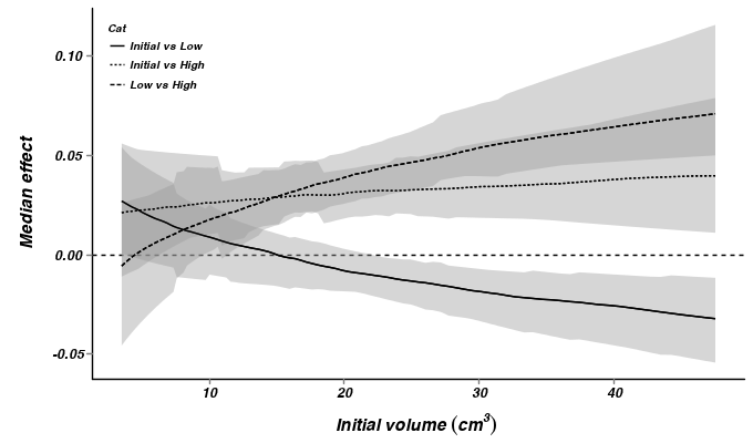
>
>
> constable.mcmc.sum <- constable.mcmc %*% t(constable.mmat)
>
> cc <- cbind(newdata, t(constable.mcmc.sum))
>
> ## initial vs low
> cc.ivl <- cbind(Cat = "Initial vs Low", ddply(cc[, 1:100], ~cIv3,
+     function(x) {
+         x1 <- apply(x[1:2, c(-1, -2)], 2, diff)
+         data.frame(mean = mean(x1), median = median(x1), coda:::HPDinterval(as.mcmc(x1),
+             p = 0.68), coda:::HPDinterval(as.mcmc(x1)))
+     }))
>
> ## initial vs high
> cc.ivh <- cbind(Cat = "Initial vs High", ddply(cc[, 1:100], ~cIv3,
+     function(x) {
+         x1 <- apply(x[c(1, 3), c(-1, -2)], 2, diff)
+         data.frame(mean = mean(x1), median = median(x1), coda:::HPDinterval(as.mcmc(x1),
+             p = 0.68), coda:::HPDinterval(as.mcmc(x1)))
+     }))
>
> ## low vs high
> cc.lvh <- cbind(Cat = "Low vs High", ddply(cc[, 1:100], ~cIv3, function(x) {
+     x1 <- apply(x[c(2, 3), c(-1, -2)], 2, diff)
+     data.frame(mean = mean(x1), median = median(x1), coda:::HPDinterval(as.mcmc(x1),
+         p = 0.68), coda:::HPDinterval(as.mcmc(x1)))
+ }))
>
> cc.all <- rbind(cc.ivl, cc.ivh, cc.lvh)
> p3 <- ggplot(data = cc.all, aes(y = median, x = cIv3, group = Cat)) +
+     geom_hline(yintercept = 0, linetype = "dashed") + geom_smooth(aes(y = median,
+     ymin = lower.1, ymax = upper.1, x = cIv3, linetype = Cat), colour = "black",
+     stat = "identity", show_guide = FALSE) + geom_smooth(aes(y = median, x = cIv3,
+     linetype = Cat), colour = "black", stat = "identity", se = FALSE) + #geom_smooth(aes(ymin=lower.1, ymax=upper.1,
+ #   linetype=Cat),colour='black',stat='identity', show_guide=FALSE)+
+ #geom_smooth(aes(linetype=Cat),colour='black',stat='identity', se=FALSE)+
+ scale_y_continuous("Median effect") + scale_x_continuous(expression(paste("Initial volume ",
+     (cm^3), "\n", sep = "")), trans = trans_new("center", transform = function(x) {
+     x1 <- x + iv3.mean
+     x1^3
+ }, inverse = function(x) {
+     x1 <- x^(1/3)
+     x2 <- x1 - iv3.mean
+ }), breaks = trans_breaks(function(x) {
+     (x + iv3.mean)^3
+ }, function(x) {
+     (x^(1/3)) - iv3.mean
+ }), labels = trans_format(function(x) {
+     (x + iv3.mean)^3
+ }, format = format_format())) + murray_opts + opts(legend.position = c(0, 1),
+     legend.justification = c(0, 1))
>
> p3
- From the multiplicative model - heterogeneous slopes