Tutorial 1 - Introduction to R
07 Mar 2017
Installing R
The latest version of an R installation binary (or source code) can be downloaded from one of the Comprehensive R Archive Network (or CRAN) mirrors. Having selected one of the (Australian) mirrors, follow one of the sets of instructions below (depending on your operating system).
- From the list of precompiled binaries, select 'Windows'
- Select the 'base' subdirectory
- Click on 'Download R_3.XX.X for Windows' (where XX.X is the current version number and release).
- Depending on the version of Windows you are running (XP, Vista or Windows 7), run (execute) this downloaded install binary. Note, if you are running Vista, you should execute this binary as Administrator. This ensures that R is installed in the system area (c:\Program Files) rather than in the user space which can lead to issues.
- Under Vista or Windows 7, when warned of either 'unidentified publisher' or 'unknown publisher' respectively, elect to allow or continue
- The installer is fairly straight forward and will guide you through the installation. The default options are typically adequate.
- Startup menus and a desktop icon will be generated

- From the list of precompiled binaries, select 'MacOS X'
- Click on 'R-3.XX.X.pkg' (where XX.X is the current version number and release) to download the installer package. Note, this is for MacOS X 10.5 (Leopard) and 10.6 (Snow Leapard) only. For earlier versions of MacOSX, you will need to scroll down to the link to 'old'
- Run the installer (double click on the image in the new finder window)
- If you are not already logged in as Administrator, you will be prompted for the Administrator password
- The installer is fairly straight forward and will guide you through the installation. The default options are typically adequate.
- From the list of precompiled binaries, select 'Linux'
- R is available in range of pre-compiled binaries for Debian (Ubuntu), Red Hat and SuSE based distributions
- Quite frankly, if you are a linux user, you do not require instructions!
Basic Syntax
The R environment and command line
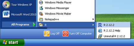
- Double click on the RGui icon on the desktop
- Click the START button from the Windows task bar
- Click Program Files
- Click R3.XX.X (where XX.X is the version and release numbers)
- Click RGui (Gui stands for Graphics User Interface)
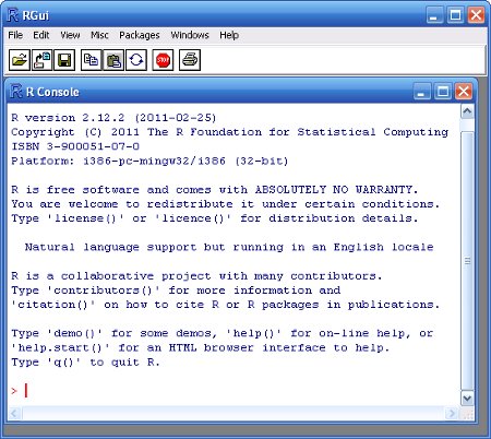
Upon opening R, you are presented with the R Console along with the command prompt (>). R is a command driven application (as opposed to a 'point-and-click' application) and despite the steep learning curve, there are many very good reasons for this.
Commands that you type are evaluated once the Enter key has been pressed
Enter the following command (5+1) at the command prompt (>);
5+1
[1] 6
Note, I have suppressed the command prompt from almost all code blocks throughout these workshop and tutorial series to make it easier for you to cut and paste code into your own scripts or directly into R.
In this tutorial series, the R code to be entered appears to the right hand side of the green bar. The number of the left side of the green bar is a line number. For single line code snippets, such as the example above, line numbers are not necessary. However, for multi-line code snippets, line numbers help for identifying and describing different parts of the code.
The above R code evaluates the command five plus one and returns the result (six).. The [1] before the 6 indicates that the object immediately to its right is the first element in the returned object. In this case there is only one object returned. However, when a large set of objects (e.g. numbers) are returned, each row will start with an index number thereby making it easier to count through the elements.
- Object
- As an object oriented language, everything in R is an object. Data, functions even output are objects.
- Vector
- A collection of one or more objects of the same type (e.g. all numbers or all characters).
- Function
- A set of instructions carried out on one or more objects. Functions are typically wrappers for a sequence of instructions that perform specific and common tasks.
- Parameter
- The kind of information passed to a function.
- Argument
- The specific information passed to a function.
- Operator
- A symbol that has a pre-defined meaning. Familiar operators include + - * and /.
Assignment operators <- Assigning a name to an object = Used when defining and specifying function arguments Logical operators (return TRUE or FALSE) Less than Greater than <= Less than or equal >= Greater than or equal == Is the left hand side equal to the right hand side (a query) != Is the left hand side NOT equal to the right hand side (a query) && Are BOTH left hand and right hand conditions TRUE || Are EITHER the left hand OR right hand conditions TRUE
Expressions, Assignment and Arithmetic
Instead of evaluating a statement and printing the result directly to the console, the results of evaluations can be stored in an object via a process called 'Assignment'. Assignment assigns a name to an object and stores the result of an evaluation in that object. The contents of an object can be viewed (printed) by typing the name of the object at the command prompt and hitting Enter.
VAR1 <- 2 + 3
VAR1
[1] 5
A single command (statement) can spread over multiple lines. If the Enter key is pressed before R considers the statement complete, the next line in the console will begin with the prompt + indicating that the statement is not complete.
> VAR2 <-
+ 2+3
> VAR2
[1] 5
Note, in the example above, I have included the command prompt so as to highlight the appearance of an incomplete expression
When the contents of an object are numbers, standard arithmetic applies;
VAR2- 1
[1] 4
ANS1 <- VAR1 * VAR2
ANS1
[1] 25
Objects can be concatenated (joined together) to create objects with multiple entries. Object concatenation is performed using the c() function.
c(1,2,6)
[1] 1 2 6
c(VAR1,VAR2)
[1] 5 5
In addition to the typical addition, subtraction, multiplication and division operators, there are a number of special operators, the simplest of which are the quotient or integer divide operator (%/%) and the remainder or modulus operator (%%).
7/3
[1] 2.333333
7%/%3
[1] 2
7%%3
[1] 1
Operator precedence
The rules of operator precedence are listed (highest to lowest) in the following table. Additionally, expressions within parentheses '()' always have highest precedence.
| Operator | Description |
|---|---|
| [ [[ | indexing |
| :: | namespace |
| $ | component |
| ^ | exponentiation (evaluated right to left) |
| - + | sign (unary) |
| : | sequence |
| %special% | special operators (e.g. %/%, %%, %*%, %in%) |
| * / | multiplication and division |
| + - | addition and subtraction |
| > < >= <= == != | ordering and comparison |
| ! | logical negation (not) |
| & && | logical AND |
| | || | logical OR |
| ~ | formula |
| -> ->> | assignment (left to right) |
| = | argument assignment (right to left) |
| <- <<- | assignment (right to left) |
| ? | help |
Command history
Each time a command is entered at the R command prompt, the command is also added to a list known as the command history. The up and down arrow keys scroll backward and forward respectively through the session's command history list and place the top most command at the current R command prompt. Scrolling through the command history enables previous commands to be rapidly re-executed, reviewed or modified and executed.
Object names
Everything created within R are objects. Objects are programming constructs that not only store values (the visible part of an object), they also define other properties of the object (such as the type of information contained in the object) and sometimes they also define certain routines that can be used to store, retrieve and manipulate data within the object.
Importantly, all objects within R must have unique names to which they can be referred. Names given to any object in R can comprise virtually any sequence of letters and numbers providing that the following rules are adhered to:
- Names must begin with a letter (names beginning with numbers or operators are not permitted)
- Names cannot contain the following characters; space , - + * / # % & [ ] { } ( ) ~
Whilst the above rules are necessary, the following naming conventions are also recommended:
- Avoid names that are the names of common predefined functions as this can provide a source of confusion for both you and R. For example, to represent the mean of a head length variable, use something like MEAN.HEAD.LENGTH or MeanHeadLength rather than mean (which is the name of a predefined function within R that calculates the mean of a set of numbers).
- In R, all commands are case sensitive and thus A and a are different and refer to different objects. Almost all inbuilt names in R are in lowercase. Therefore, one way to reduce the likelihood of assigning a name that is already in use by an inbuilt object is to only use uppercase names for any objects that you create. In practice, having at least one uppercase letter in the name (provided it is not the first letter) is typically sufficient to avoid name clashes.
- Names should reflect the content of the object. One of the powerful features of R is that there is virtually no limit to the number of objects (variables, datasets, results, models, etc) that can be in use at a time. However, without careful name management, objects can rapidly become misplaced or ambiguous. Therefore, the name of an object should reflect what it is, and what has happened to it. For example, the name Log.FISH.WTS might be given to an object that contains log transformed fish weights. Moreover, many prefer to prefix the object name with a lowercase letter that denotes the type of data containing in the object. For example, dMeanHeadLength might indicate that the object contains the mean head lengths stored as a double floating point (real numbers).
- Although there are no restrictions on the length of names, shorter names are quicker to type and provide less scope for typographical errors and are therefore recommended (of course within the restrictions of the point above).
- Separate any words in names by a decimal point or an underscore (if not using camel case). For example, HEAD.LENGTH, HEAD_LENGTH might be used to represent a numeric vector of head lengths
R Sessions and Workspaces
A number of objects have been created in the current session (a session encapsulates all the activity since the current instance of the R application was started). To review the names of all of the objects in the users current workspace (storage of user created objects);
ls()
[1] "ANS1" "my_png" "VAR1" "VAR2"
From the above output, ignore the elements 'printVerbatim', 'Routput' and 'SweaveSyntaxHTML' - they are objects that are involved in the production of this web-page! Note, the [5] indicating that the second row of output starts with the fifth element of the output.
You can also refine the scope of the ls() function to search for object names that match a pattern;
ls(pat="VAR")
[1] "VAR1" "VAR2"
ls(pat="A*1")
[1] "ANS1" "VAR1"
The longer the session is running, the more objects will be created resulting in a very cluttered workspace. Unneeded objects can be removed using the rm() function;
rm(VAR1,VAR2)  #remove the VAR1 and VAR2 objects
rm(list=ls())  #remove all user defined objects
Current working directory
The R working directory (location from which files/data are read and written) is by default, the location of the R executable (or execution path in Linux). The current working directory can be reviewed and changed (for the session) using the getwd() function and setwd() function respectively. Note that R uses the Unix/Linux style directory subdivision markers. That is, R uses the forward slash / in path names rather than the regular \ of Windows.
setwd("~/Work/")  #change the current working directory path
getwd()  #review the current working directory
[1] "/home/murray/Work"
list.files(path=getwd()) #list all files (and directories) in the current working directory
[1] "SUYR"
Workspaces
Throughout an R session, all objects (including loaded packages, see section 1.19) that have been added are stored within the R global environment, called the workspace. Occasionally, it is desirable to save the workspace and thus all those objects (vectors, functions, etc) that were in use during a session so that they are automatically available during subsequent sessions. This can be done using the save.image() function. Note, this will save the workspace to a file called .RData in the current working directory (usually the R startup directory), unless a filename (and path) is supplied as an argument to the save.image() function. A previously saved workspace can be loaded by providing a full path and filename as an argument to the load() function. Whilst saving a workspace image can sometimes be convenient, it can also contribute greatly to organizational problems associated with large numbers of obsolete or undocumented objects. Instead, it is usually better to specifically store each of the objects you know you are going to want to have access to across sessions separately.
Quitting elegantly
To quit R, issue the following command; Note in Windows and MacOSX, the application can also be terminated using the standard Exiting protocols.
q()
You will then be asked whether or not you wish to save the current workspace. If you do, enter 'Y' otherwise enter 'N'. Unless you have a very good reason to save the workspace, I would suggest that you do not. A workspace generated in a typical session will have numerous poorly named objects (objects created to temporarily store information whilst testing). Next time R starts, it could restore this workspace thereby starting with a cluttered workspace, but becoming a potential source of confusion if you inadvertently refer to an object stored during a previous session.
Functions
As wrappers for collections of commands used together to perform a task, functions provide a convenient way of interacting with all of these commands in sequence. Most functions require one or more inputs (parameters), and while a particular function can have multiple parameters, not all are necessarily required (some could have default values). Parameters are parsed to a function as an argument comprising the name of the parameter, an equals operator and the value of the parameter. Hence, arguments are specified as name, value pairs.
Consider the seq() function, which generates a sequence of values (a vector) according to the values of the arguments. This function has the following definition;
- If the seq() function is called without any arguments (e.g. seq()), it will return a single number 1. Using the default arguments for the function, it returns a vector starting at 1 (from=1), going up to 1 (to=1) and thus having a length of 1.
- We can alter this behavior by specifically providing values for the named arguments. The following generates a sequence of numbers from 2 to 10 incrementing by 1 (default);
- The following generates a sequence of numbers from 2 to 10 incrementing by 2;
- Alternatively, instead of manipulating the increment space of the sequence, we could specify the desired length of the sequence;
- Named arguments need not include the full name of the parameter, so long as it is unambiguous which parameter is being referred to. For example, length.out could be shortened to just l since there are no other parameters of this function that start with 'l';
- Parameters can also be specified as unnamed arguments provided they are in the order specified in the function definition. For example to generate a sequence of numbers from 2 to 10 incrementing by 2;
- Named and unnamed arguments can be mixed, just remember the above rules about parameter order and unambiguous names;
seq(from=2,to=10)
[1] 2 3 4 5 6 7 8 9 10
seq(from=2,to=10,by=2)
[1] 2 4 6 8 10
seq(from=2,to=10,length.out=3)
[1] 2 6 10
seq(from=2,to=10,l=4)
[1] 2.000000 4.666667 7.333333 10.000000
seq(2,10,2)
[1] 2 4 6 8 10
seq(2,10,l=4)
[1] 2.000000 4.666667 7.333333 10.000000
Function overloading (polymorphism)
Many routines can be applied to different sorts of data. That is, they are somewhat generic. For example, we could calculate the mean (arithmetic center) of a set of numbers or we could calculate the mean of a set of dates or times. Whilst the calculations in both cases are analogous to one another, they nevertheless differ sufficiently so as to warrant separate functions.
We could name the functions that calculate the mean of a set of numbers and the mean of a set of dates as mean.numbers and mean.dates respectively. Unfortunately, as this is a relatively common situation, the number of functions to learn rapidly expands. And from the perspective of writing a function that itself contains such a generic function, we would have to write multiple instances of the function in order to handle all the types of data we might want to accommodate.
To simplify the process of applying these generic functions, R provides yet another layer that is responsible for determining which of a series of overloaded functions is likely to be applicable according to the nature of the parameters and data parsed as arguments to the function. To see this in action, type mean followed by hitting the TAB key. The TAB key is used for auto-completion and therefore this procedure lists all the objects that begin with the letters 'mean'.
mean 	 mean.Date 	 mean.default 	 mean.difftime
 mean.POSIXct 	 mean.POSIXlt 	 mean
In addition to an object called 'mean, there are additional objects that are suffixed as a '.' followed by a data type. In this case, the objects mean.default, mean.Date, mean.POSIXct, mean.POSIXlt, mean.difftime and mean.data.frame are functions that respectively calculate the mean of a set of numbers, dates, times, times, time differences and data frame columns. The mean function determines which of the other functions is appropriate for the data parsed and then redirects to that appropriate function. Typically, this means that it is only necessary to remember the one generic function (in this case, mean()).
# mean of a series of numbers
mean(c(1,2,3,4))
[1] 2.5
# create a sequence of dates spaced 7 days apart between 29th Feb 2000 and 30th Apr 2000
sampleDates <- seq(from=as.Date("2000-02-29"),to=as.Date("2000-04-30"), by="7 days")
# print (view) these dates
sampleDates
[1] "2000-02-29" "2000-03-07" "2000-03-14" "2000-03-21" "2000-03-28" "2000-04-04" "2000-04-11"
[8] "2000-04-18" "2000-04-25"
# calculate the mean of these dates
mean(sampleDates)
[1] "2000-03-28"
In the above examples, we called the same function (mean) on both occasions. In the first instance, it was equivalent to calling the mean.default() function and in the second instance the mean.Date() function. Note that the seq() function is similarly overloaded.
The above example also illustrates another important behaviour of function arguments. Function calls can be nested within the arguments of other functions and function arguments are evaluated before the function runs. In this way, multiple steps to be truncated together (although for the sake of the codes' readability and debugging, it is often better to break a problem up into smaller steps). If a function argument itself contains a function (as was the case above with the from= and to= arguments, both of which called the as.Date() function which converts a character string into a date object), the value of the evaluated argument is parsed to the outside function. That is, evaluations are made from the inside to out. The above example, could have been further truncated to;
# calculate the mean of a sequence of dates spaced 7 days apart between 29th Feb 2000 and 30th Apr 2000
mean(seq(from=as.Date("2000-02-29"),to=as.Date("2000-04-30"), by="7 days"))
[1] "2000-03-28"
External functions
As R is a scripting language (rather than a compiled language), it has the potential to be very slow (since syntax checking, machine instruction interpretation, etc must all take place at runtime rather than at compile time). Consequently, many of the functions are actually containers (wrappers) for external code (link libraries) precompiled in either C or Fortran. In this way, the environment can benefit from the flexibility of a scripting language whilst still maintaining most of the speed of a compiled language. Tutorial 4 will introduce how to write, compile and link to external libraries as part of a tutorial on R programming.
Getting help
There are numerous ways of seeking help on R syntax and functions (the following all ways of finding information about a function that calculates the mean of a vector).
- Providing the name of the function as an argument to the help(mean)function
help(mean)
- Typing the name of the function preceded by a '?'
?mean
- To run the examples within the standard help files, use the example() function
example(mean)
- Some packages include demonstrations that showcase their features and use cases. The demo() function provides a user-friendly way to access these demonstrations. For example, to respectively get an overview of the basic graphical procedures in R and get a list of available demonstrations;
Note in the above example everything following the # (comment character) is ignored. This provides a way of including comments.
demo(graphics)  #run the graphics demo
demo()          #list all demos available on your system
- If you don't know the exact name of the function, the apropos() function is useful as it returns the name of all objects from the current search list that match a specific pattern;
apropos('mea')
 [1] "colMeans"           ".colMeans"          "influence.measures" "kmeans"
 [5] "mean"               "mean.Date"          "mean.default"       "mean.difftime"
 [9] "mean.POSIXct"       "mean.POSIXlt"       "Meat"               "rowMeans"
[13] ".rowMeans"          "weighted.mean"
- If you have no idea what the function is called, the help.search() and help.start() functions search through the regular manuals and the local HTML manuals (via a web browser) respectively for specific terms;
help.search('mean')  #search the local R manuals
help.start()          #search the local HTML R manuals
- To get a snapshot of the order and default values of a functions' arguments, use the args() function;
args(mean) #the arguments that apply to the mean function
function (x, ...)
NULL
args(list.files) #the arguments that apply to the list.files function
function (path = ".", pattern = NULL, all.files = FALSE, full.names = FALSE,
    recursive = FALSE, ignore.case = FALSE, include.dirs = FALSE,
    no.. = FALSE)
NULL
Data Types
Vectors
Vectors are a collection of one or more entries (values) of the same type (class) and are the basic storage unit in R. Vectors are one-dimensional arrays (have a single dimension - length) and can be thought of as a single column of data. Each entry in a vector has a unique index (like a row number) to enable reference to particular entries in the vector.
The c() function
The c() function concatenates values together into a vector. To create a vector with the numbers 1, 4, 7, 21;
c(1,4,7,21)
[1] 1 4 7 21
As an example, we could store the temperature recorded at 10 sites;
TEMPERATURE <- c(36.1, 30.6, 31, 36.3, 39.9, 6.5, 11.2, 12.8, 9.7, 15.9)
TEMPERATURE
[1] 36.1 30.6 31.0 36.3 39.9 6.5 11.2 12.8 9.7 15.9
To create a vector with the words 'Fish', 'Rock', 'Tree', 'Git';
c('Fish', 'Rock', 'Tree', "Git")
[1] "Fish" "Rock" "Tree" "Git"
Regular or patterned sequences
We have already seen the use of the seq() function to create sequences of entries.
Sequences of repeated entries are supported with the rep() function;
rep(4,5)
[1] 4 4 4 4 4
rep('Fish',5)
[1] "Fish" "Fish" "Fish" "Fish" "Fish"
The paste() function
To create a sequence of quadrat labels we could use the c() function as illustrated above,e.g.
QUADRATS <- c("Q1","Q2","Q3","Q4","Q5","Q6","Q7","Q8","Q9","Q10")
QUADRATS
[1] "Q1" "Q2" "Q3" "Q4" "Q5" "Q6" "Q7" "Q8" "Q9" "Q10"
A more elegant way of doing this is to use the paste() function;
QUADRATS <- paste("Q",1:10,sep="")
QUADRATS
[1] "Q1" "Q2" "Q3" "Q4" "Q5" "Q6" "Q7" "Q8" "Q9" "Q10"
This can be useful for naming vector elements. For example, we could use the names() function to name the elements of the temperature variable according to the quadrat labels.
names(TEMPERATURE) <- QUADRATS
TEMPERATURE
  Q1   Q2   Q3   Q4   Q5   Q6   Q7   Q8   Q9  Q10
36.1 30.6 31.0 36.3 39.9  6.5 11.2 12.8  9.7 15.9
The paste() function can also be used in conjunction with other functions to generate lists of labels. For example, we could combine a vector in which the letters A, B, C, D and E (generated with the LETTERS constant) are each repeated twice consecutively (using the rep() function) with a vector that contains a 1 and a 2 to produce a character vector that labels sites in which the quadrats may have occurred.
SITE <- paste(rep(LETTERS[1:5], each = 2), 1:2, sep = "")
SITE
[1] "A1" "A2" "B1" "B2" "C1" "C2" "D1" "D2" "E1" "E2"
| Vector Class | Example |
|---|---|
| integer (whole numbers) | > 2:4 [1] 2 3 4 > c(1,3,9) [1] 1 3 9 |
| numeric (real numbers) | > c(8.4, 2.1) [1] 8.4 2.1 |
| character (letters) | > c('A', 'ABC') [1] "A" "ABC" |
| logical (TRUE or FALSE) | > c(2:4)==3 [1] FALSE TRUE FALSE |
| date (dates) | > c(as.Date("2000-02-29"), as.Date("29/02/2000","%d/%m/%Y")) [1] "2000-02-29" "2000-02-29" |
| POSIXlt (date-time) | > strptime('2011-03-27 01:30:00', format='%Y-%m-%d %H:%M:%S') [1] "2011-03-27 01:30:00" |
Factors
Factors are more than a vector of characters. Factors have additional properties that are utilized during statistical analyses and graphical procedures. To illustrate the difference, we will create a vector to represent a categorical variable indicating the level of shading applied to 10 quadrats. Firstly, we will create a character vector;
SHADE <- rep(c("no","full"),each=5)
SHADE
[1] "no" "no" "no" "no" "no" "full" "full" "full" "full" "full"
Now we convert this into a factor;
SHADE <- factor(SHADE)
SHADE
 [1] no   no   no   no   no   full full full full full
Levels: full no
Notice the additional property (Levels) at the end of the output. Notice also that unless specified otherwise, the levels are ordered alphabetically. Whilst this does not impact on analyses, it does effect interpretations and graphical displays. If the alphabetical ordering does not reflect the natural order of the data, it is best to reorder the levels whilst defining the factor;
SHADE <- factor(SHADE, levels=c("no","full"))
SHADE
 [1] no   no   no   no   no   full full full full full
Levels: no full
A more convenient way to create a balanced (equal number of replicates) factor is to use the gl() function. To create the shading factor from above;
SHADE <- gl(2,5,10,c("no","full"))
SHADE
 [1] no   no   no   no   no   full full full full full
Levels: no full
Matrices
Matrices have two dimensions (length and width). The entries (which must be all of the same length and type - class) are in rows and columns.
We could arrange the vector of shading into two columns;
matrix(TEMPERATURE,nrow=5)
     [,1] [,2]
[1,] 36.1  6.5
[2,] 30.6 11.2
[3,] 31.0 12.8
[4,] 36.3  9.7
[5,] 39.9 15.9
Similarly, We could arrange the vector of shading into two columns;
matrix(SHADE,nrow=5)
     [,1] [,2]
[1,] "no" "full"
[2,] "no" "full"
[3,] "no" "full"
[4,] "no" "full"
[5,] "no" "full"
As another example, we could store the X,Y coordinates for five quadrats within a grid. We start by generating separate vectors to represent the X and Y coordinates and then we bind them together using the cbind() function (which combines objects by columns);
X <- c(16.92,24.03,7.61,15.49,11.77)
Y<- c(8.37,12.93,16.65,12.2,13.12)
XY <- cbind(X,Y)
XY
         X     Y
[1,] 16.92  8.37
[2,] 24.03 12.93
[3,]  7.61 16.65
[4,] 15.49 12.20
[5,] 11.77 13.12
rbind(X,Y)
   [,1]  [,2]  [,3]  [,4]  [,5]
X 16.92 24.03  7.61 15.49 11.77
Y  8.37 12.93 16.65 12.20 13.12
We could even alter the row names;
rownames(XY) <- LETTERS[1:5]
XY
      X     Y
A 16.92  8.37
B 24.03 12.93
C  7.61 16.65
D 15.49 12.20
E 11.77 13.12
Importantly, all entries in a matrix must be of the same type. That is, they must all be numeric, or all be characters etc. If we attempt to mix a combination of data types in a matrix, then the data will all be converted into a type that can accommodate all the data. For example, if we attempt to bind together the numeric TEMPERATURE data and the character SITE data into a matrix, then the result will be a matrix of characters (since while it is possible to covert numbers to strings, in this case the reverse is not possible).
cbind(TEMPERATURE,SITE)
    TEMPERATURE SITE
Q1  "36.1"      "A1"
Q2  "30.6"      "A2"
Q3  "31"        "B1"
Q4  "36.3"      "B2"
Q5  "39.9"      "C1"
Q6  "6.5"       "C2"
Q7  "11.2"      "D1"
Q8  "12.8"      "D2"
Q9  "9.7"       "E1"
Q10 "15.9"      "E2"
On the other hand, if we attempt to bind together the numeric TEMPERATURE data and the factor SHADE data into a matrix, then the result will be a matrix of numbers (recall that factors are internally stored as integers, yet they have a levels property that acts rather like a lookup key).
cbind(TEMPERATURE,SHADE)
    TEMPERATURE SHADE
Q1         36.1     1
Q2         30.6     1
Q3         31.0     1
Q4         36.3     1
Q5         39.9     1
Q6          6.5     2
Q7         11.2     2
Q8         12.8     2
Q9          9.7     2
Q10        15.9     2
Lists
Lists provide a way to group together multiple objects of different type and length. For example, whilst the contents of any single vector or matrix must all be of the one type and length (e.g. all numeric or all character), a list can contain any combination of vectors, matrices, scalars and of any type. Furthermore, the objects contained in a list do not need to be of the same lengths (c.f data frames). The output of most analyses are returned as lists.
As an example, we could group together the previously created isolated vectors and matrices into a single object that encapsulates the entire experiment;
EXPERIMENT <- list(SITE=SITE,QUADRATS = QUADRATS,COORDINATES = XY, SHADE = SHADE, TEMPERATURE = TEMPERATURE)
EXPERIMENT
$SITE
 [1] "A1" "A2" "B1" "B2" "C1" "C2" "D1" "D2" "E1" "E2"

$QUADRATS
 [1] "Q1"  "Q2"  "Q3"  "Q4"  "Q5"  "Q6"  "Q7"  "Q8"  "Q9"  "Q10"

$COORDINATES
      X     Y
A 16.92  8.37
B 24.03 12.93
C  7.61 16.65
D 15.49 12.20
E 11.77 13.12

$SHADE
 [1] no   no   no   no   no   full full full full full
Levels: no full

$TEMPERATURE
  Q1   Q2   Q3   Q4   Q5   Q6   Q7   Q8   Q9  Q10
36.1 30.6 31.0 36.3 39.9  6.5 11.2 12.8  9.7 15.9
Lists can be thought of as a set of objects bound into a single container. In the example above, the list object EXPERIMENT contains a copy of the SITE, QUADRATS, COORDINATES, SHADE and TEMPERATURE objects.
Importantly, once a list has been created the objects within the list are not linked in any way to the original objects from which the list is formed. Consequently, any changes made to (for example) the TEMPERATURE object will not be reflected in the content of the TEMPERATURE object within the EXPERIMENT list.
To access an object within a list, the $ operator is used as such:
EXPERIMENT$TEMPERATURE
  Q1   Q2   Q3   Q4   Q5   Q6   Q7   Q8   Q9  Q10
36.1 30.6 31.0 36.3 39.9  6.5 11.2 12.8  9.7 15.9
Dataframes - data sets
Rarely are single biological variables collected in isolation. Rather, data are usually collected in sets of variables reflecting investigations of patterns between and/or among the different variables. Consequently, data sets are best organized into matrices of variables (vectors) all of the same lengths yet not necessarily of the same type. Hence, neither lists nor matrices represent natural storages for data sets. This is the role of data frames which are used to store a set of vectors of the same length (yet potentially different types) in a rectangular matrix.
Data frames are generated by combining multiple vectors together such that each vector becomes a separate column in the data frame. For a data frame to faithfully represent a data set, the sequence in which observations appear in the vectors must be the same for each vector, and each vector should have the same number of observations. For example, the first, second, third...etc entries in each vector must represent respectively, the observations collected from the first, second, third...etc sampling units.
Since the focus of these tutorials is on the exploration, analysis and summary of data sets, and data sets are accommodated in R by data frames, the generation, importation, exportation, manipulation and management of data frames receives extensive coverage in tutorials 2.1, 2.2, 2.3, 2.4 and 2.5.
As an example of a data frame, we could again group together the previously created isolated vectors into a single object that encapsulates a data set;
DATA <- data.frame(SITE=SITE,QUADRATS = QUADRATS, SHADE = SHADE, TEMPERATURE = TEMPERATURE)
DATA
    SITE QUADRATS SHADE TEMPERATURE
Q1    A1       Q1    no        36.1
Q2    A2       Q2    no        30.6
Q3    B1       Q3    no        31.0
Q4    B2       Q4    no        36.3
Q5    C1       Q5    no        39.9
Q6    C2       Q6  full         6.5
Q7    D1       Q7  full        11.2
Q8    D2       Q8  full        12.8
Q9    E1       Q9  full         9.7
Q10   E2      Q10  full        15.9
Object Manipulation
Object information
As indicated earlier, everything in R is an object. All objects have a type or class that encapsulates the sort of information stored in the object as well as determining how other functions interact with the object. The class of an object can be reviewed with the class() function;
class(TEMPERATURE)
[1] "numeric"
class(DATA)
[1] "data.frame"
class(mean)
[1] "function"
There is also a family of functions prefixed with is. that evaluate whether or not an object is of a particular class (or type) or not. The following table lists the common object query functions. All object query functions return a logical vector. Enter methods(is) for a more comprehensive list.
| Function | Returns TRUE: | Example |
|---|---|---|
| is.numeric(x) | if all elements of x are numeric or integer | is.numeric(c(1,-3.5, TEMPERATURE)) |
| is.null(x) | if x is null (the object has no length) | is.null(NULL) |
| is.logical(x) | if all elements of x are logical | is.logical(c(TRUE,TRUE)) |
| is.character(x) | if all elements of x are character strings | is.character(c("A","Plant",QUADRATS)) |
| is.vector(x) | if the object x is a vector (has only a single dimension). Returns FALSE if object has attributes other than names. | is.vector(TEMPERATURE) |
| is.factor(x) | if the object x is a factor | is.factor(SHADE) |
| is.matrix(x) | if the object x is a matrix (two dimensions, yet not a data.frame | is.matrix(XY) |
| is.list(x) | if the object x is a list | is.list(EXPERIMENT) |
| is.data.frame(x) | if the object x is a data.frame | is.data.frame(DATA) |
| is.na(x) | for each missing (NA) element in x | is.na(c(NA,NA)) |
| ! | ('not') operator as a prefix converts the above functions into 'is.not' | !is.factor(DATA) |
Attributes
Many R objects also have a set of attributes, the number and type of which are specific to each class of object. For example, a matrix object has a specific number of dimensions as well as row and column names. The attributes of an object can be viewed using the attributes() function:
attributes(XY)
$dim
[1] 5 2

$dimnames
$dimnames[[1]]
[1] "A" "B" "C" "D" "E"

$dimnames[[2]]
[1] "X" "Y"
Similarly, the attr() function can be used to view and set individual attributes of an object, by specifying the name of the object and the name of the attribute (as a character string) as arguments. For example:
attr(XY, "dim")
[1] 5 2
attr(XY, "description") <- "coordinates of quadrats"
XY
      X     Y
A 16.92  8.37
B 24.03 12.93
C  7.61 16.65
D 15.49 12.20
E 11.77 13.12
attr(,"description")
[1] "coordinates of quadrats"
Note that in the above example, the attribute 'description' is not a inbuilt attribute of a matrix. When a new attribute is set, this attribute is displayed along with the object. This provides a useful way of attaching a description to an object, thereby reducing the risks of the object becoming unfamiliar.
Object conversion
Objects can be converted or coerced into other objects using a family of functions with a as. prefix. Note that there are some obvious restrictions on these conversions as most objects cannot be completely accommodated by all other object types, and therefore some information (such as certain attributes) may be lost or modified during the conversion. Objects and elements that cannot be successfully coerced are returned as NA. The following table lists the common object coercion functions. Use methods(as) for a more comprehensive list.
| Function | Converts object to |
|---|---|
| as.numeric(x) | a numeric vector ('integer' or 'real'). Factors converted to integers. |
| as.null(x) | a NULL |
| as.logical(x) | a logical vector. A values of >1 converted to TRUE otherwise FALSE. |
| as.character(x) | a character (string) vector. |
| as.vector(x) | a vector. All attributes (including names) are removed. |
| as.factor(x) | a factor. This is an abbreviated (with respect to its argument set) version of the factor() function. |
| as.matrix(x) | a matrix. Any non-numeric elements result in all matrix elements being converted to characters. |
| as.list(x,) | a list. |
| as.data.frame(x,) | a data.frame. Matrix columns and list items are converted into separate vectors of the dataframe and character vectors are converted into factors. All previous attributes are removed. |
| as.Date(x) | a date. |
Indexing
Indexing is the means by which data are filtered (subsetted) to include and exclude certain entries.
Vector indexing
Subsets of vectors are produced by appending an index vector (inclosed in square brackets []) to a vector name. There are four common forms of vector indexing used to extract a subset of vectors
- Vector of positive integers - a set of integers that indicate which elements of the vector should be included;
- Vector of negative integers - a set of integers that indicate which elements of the vector should be excluded;
- Vector of character strings (referencing names) - for vectors whose elements have been named, a vector of names can be used to select elements to include;
- Vector of logical values - a vector of logical values (TRUE or FALSE) the same length as the vector being subsetted. Entries corresponding to a logical TRUE are included, FALSE are excluded;
TEMPERATURE[2]
  Q2
30.6
TEMPERATURE[2:5]
  Q2   Q3   Q4   Q5
30.6 31.0 36.3 39.9
TEMPERATURE[c(1,5,6,9)]
  Q1   Q5   Q6   Q9
36.1 39.9  6.5  9.7
TEMPERATURE[-2]
  Q1   Q3   Q4   Q5   Q6   Q7   Q8   Q9  Q10
36.1 31.0 36.3 39.9  6.5 11.2 12.8  9.7 15.9
TEMPERATURE[c(1,5,6,9)*-1]
  Q2   Q3   Q4   Q7   Q8  Q10
30.6 31.0 36.3 11.2 12.8 15.9
TEMPERATURE["Q1"]
  Q1
36.1
TEMPERATURE[c("Q1","Q4")]
  Q1   Q4
36.1 36.3
TEMPERATURE[TEMPERATURE < 15]
  Q6   Q7   Q8   Q9
 6.5 11.2 12.8  9.7
TEMPERATURE[SHADE == "no"]
  Q1   Q2   Q3   Q4   Q5
36.1 30.6 31.0 36.3 39.9
TEMPERATURE[TEMPERATURE < 34 & SHADE == "no"]
  Q2   Q3
30.6 31.0
TEMPERATURE[TEMPERATURE < 10 | SHADE == "no"]
  Q1   Q2   Q3   Q4   Q5   Q6   Q9
36.1 30.6 31.0 36.3 39.9  6.5  9.7
Matrix indexing
Similar to vectors, matrices can be indexed using positive integers, negative integers, character strings and logical vectors. However, whereas vectors have a single dimension (length), matrices have two dimensions (length and width). Hence, indexing needs to reflect this. It is necessary to specify both the row and column number. Matrix indexing takes of the form of [row.indices, col.indices] where row.indices and col.indices respectively represent sequences of row and column indices. If a row or column index sequence is omitted, it is interpreted as the entire row or column respectively.
XY[3,2]
[1] 16.65
XY[3,]
    X     Y
 7.61 16.65
XY[,-2]
    A     B     C     D     E
16.92 24.03  7.61 15.49 11.77
XY["A",1:2]
    X     Y
16.92  8.37
XY[,"X"]
    A     B     C     D     E
16.92 24.03  7.61 15.49 11.77
XY[XY[,"X"]>12,]
      X     Y
A 16.92  8.37
B 24.03 12.93
D 15.49 12.20
List indexing
Lists consist of collections of objects that need not be of the same size or type. The objects within a list are indexed by appending an index vector (enclosed in single or double square brackets, [] or [[]]), to the list name. Single square brackets provide access to multiple list items (returned as a list), whereas double square brackets provide access to individual list items (returned according to the type of object represented by the list item). A single object within a list can also be referred to by appending a string character ($) followed by the name of the object to the list names (e.g. list$object). The elements of objects within a list are indexed according to the object type. Vector indices to objects within other objects (lists) are placed within their own square brackets outside the list square brackets: Recall the EXPERIMENT list we generated earlier
EXPERIMENT
$SITE
 [1] "A1" "A2" "B1" "B2" "C1" "C2" "D1" "D2" "E1" "E2"

$QUADRATS
 [1] "Q1"  "Q2"  "Q3"  "Q4"  "Q5"  "Q6"  "Q7"  "Q8"  "Q9"  "Q10"

$COORDINATES
      X     Y
A 16.92  8.37
B 24.03 12.93
C  7.61 16.65
D 15.49 12.20
E 11.77 13.12

$SHADE
 [1] no   no   no   no   no   full full full full full
Levels: no full

$TEMPERATURE
  Q1   Q2   Q3   Q4   Q5   Q6   Q7   Q8   Q9  Q10
36.1 30.6 31.0 36.3 39.9  6.5 11.2 12.8  9.7 15.9
The following examples illustrate the common ways to subset (index) lists.
- A vector of positive numbers (single brackets) - that indicate which list items should be included;
EXPERIMENT[c(1,3)]
$SITE [1] "A1" "A2" "B1" "B2" "C1" "C2" "D1" "D2" "E1" "E2" $COORDINATES X Y A 16.92 8.37 B 24.03 12.93 C 7.61 16.65 D 15.49 12.20 E 11.77 13.12 - A single positive number (double brackets) - that indicates which list item should be included;
EXPERIMENT[[1]]
[1] "A1" "A2" "B1" "B2" "C1" "C2" "D1" "D2" "E1" "E2"
- A vector of character strings (single brackets) - that indicate which list items should be included;
EXPERIMENT[c('TEMPERATURE','SHADE')]
$TEMPERATURE
  Q1   Q2   Q3   Q4   Q5   Q6   Q7   Q8   Q9  Q10
36.1 30.6 31.0 36.3 39.9  6.5 11.2 12.8  9.7 15.9

$SHADE
 [1] no   no   no   no   no   full full full full full
Levels: no full
- A single character string (double brackets) - that indicates which list item should be included;
EXPERIMENT[['TEMPERATURE']]
  Q1   Q2   Q3   Q4   Q5   Q6   Q7   Q8   Q9  Q10
36.1 30.6 31.0 36.3 39.9  6.5 11.2 12.8  9.7 15.9
#OR equivalently (recall earlier)
EXPERIMENT$TEMPERATURE
  Q1   Q2   Q3   Q4   Q5   Q6   Q7   Q8   Q9  Q10
36.1 30.6 31.0 36.3 39.9  6.5 11.2 12.8  9.7 15.9
- Extract the first element of each list item - returned as a matrix;
sapply(EXPERIMENT,"[",1)
          SITE       QUADRATS    COORDINATES          SHADE TEMPERATURE.Q1
          "A1"           "Q1"        "16.92"            "1"         "36.1"
#notice that only one element of the coordinate pair is included #OR when the list items are not vectors do.call(cbind, EXPERIMENT)[1,]
       SITE    QUADRATS           X           Y       SHADE TEMPERATURE
       "A1"        "Q1"     "16.92"      "8.37"         "1"      "36.1"
#OR as a data frame (on the items that are of equal size) library(plyr) quickdf(EXPERIMENT[c(1,2,4,5)])[1,]
  SITE QUADRATS SHADE TEMPERATURE
1   A1       Q1    no        36.1
Pattern matching and replacement
An important part of filtering is the ability to detect patterns on which to base selections or exclusions. Numerical and categorical filtering rules are generally fairly straight forward, however complex filtering rules can also be devised from character vectors. Furthermore, the ability to search and replace character strings within a character vector can also be very useful.
grep - index of match
The grep() function searches within a vector for matches to a pattern and returns the index of all matching entries.
# get the indexes of elements of the SITE vector that contain an 'A'
grep(pattern="A", EXPERIMENT$SITE)
[1] 1 2
# use the results of the grep as indexes to select only those 'SITE' values that contain an 'A'
EXPERIMENT$SITE[grep(pattern="A", EXPERIMENT$SITE)]
[1] "A1" "A2"
The pattern can comprise any valid regular expression and is therefore very flexible:
# get the indexes of values of the 'SITE' vector within the DATA dataframe that contain either an 'A', 'B' or 'C' followed by a '1'
grep("[A-C]1", DATA$SITE)
[1] 1 3 5
# select only those rows of the DATA dataframe that correspond to a 'SITE' value of either an 'A', 'B' or 'C' followed by a '1'
DATA[grep("[A-C]1", DATA$SITE), ]
   SITE QUADRATS SHADE TEMPERATURE
Q1   A1       Q1    no        36.1
Q3   B1       Q3    no        31.0
Q5   C1       Q5    no        39.9
regexp - position and length of match
Rather than return the indexes of matching entries, the regexpr() function returns the position of the match within each string as well as the length of the pattern within each string (-1 values correspond to entries in which the pattern is not found).
AUST <- c("Adelaide", "Brisbane", "Canberra", "Darwin", "Hobart", "Melbourne", "Perth", "Sydney")
AUST
[1] "Adelaide" "Brisbane" "Canberra" "Darwin" "Hobart" "Melbourne" "Perth" "Sydney"
#get the position and length of string of characters containing an 'a' and an 'e' separated by any number of characters
regexpr(pattern="a.*e", AUST)
[1]  5  6  2 -1 -1 -1 -1 -1
attr(,"match.length")
[1]  4  3  4 -1 -1 -1 -1 -1
attr(,"useBytes")
[1] TRUE
gsub - pattern replacement
The gsub() function replaces all instances of an identified pattern within a character vector with an alternative set of characters. The similar sub() function replaces only the first instance.
DATA$SHADE
 [1] no   no   no   no   no   full full full full full
Levels: no full
gsub("no", "Not shaded", DATA$SHADE)
 [1] "Not shaded" "Not shaded" "Not shaded" "Not shaded" "Not shaded" "full"       "full"
 [8] "full"       "full"       "full"
It is also possible to extend the functionality to accomodate perl-compatible regular expressions.
#convert all the capital values entries into uppercase identify (and store) all words (\\w) convert stored pattern (\\1) to uppercase (\\U)
gsub("(\\w)", "\\U\\1", AUST, perl = TRUE)
[1] "ADELAIDE" "BRISBANE" "CANBERRA" "DARWIN" "HOBART" "MELBOURNE" "PERTH" "SYDNEY"
substr - extracting substrings
The substr() function is used to extract parts of string (set of characters) entries within character vectors and thus is useful for making truncated labels (particularly for graphical summaries). For example, if we had a character vector containing the names of the Australian capital cities and required abbreviations (first 3 characters) for graph labels:
#recall the AUST character vector that lists the Australian capital cities
AUST
[1] "Adelaide" "Brisbane" "Canberra" "Darwin" "Hobart" "Melbourne" "Perth" "Sydney"
substr(AUST, start=1, stop=3)
[1] "Ade" "Bri" "Can" "Dar" "Hob" "Mel" "Per" "Syd"
Alternatively, we could use the abbreviate() function.
abbreviate(AUST, minlength = 3)
 Adelaide  Brisbane  Canberra    Darwin    Hobart Melbourne     Perth    Sydney
    "Adl"     "Brs"     "Cnb"     "Drw"     "Hbr"     "Mlb"     "Prt"     "Syd"
Value matching
In addition to the above matching procedures, it is possible to compare vectors via the usual set of binary operators
(x<y, x>y, x≤y, x≥y, x==y and x!=y).
SHADE == 'no'
[1] TRUE TRUE TRUE TRUE TRUE FALSE FALSE FALSE FALSE FALSE
TEMPERATURE > 32
   Q1    Q2    Q3    Q4    Q5    Q6    Q7    Q8    Q9   Q10
 TRUE FALSE FALSE  TRUE  TRUE FALSE FALSE FALSE FALSE FALSE
# Compare 'Q1' to items 1,3,5,7,9 of QUADRATS and compare 'Q3' to items 2,4,6,8,10.
QUADRATS == c('Q1','Q3')
[1] TRUE FALSE FALSE FALSE FALSE FALSE FALSE FALSE FALSE FALSE
Warning, be very cautious when using the binary operators x==y or x!=y to compare numeric vectors as they do not allow for rounding errors or finite representation of fractions and will almost always return FALSE even for values that appear identical. As an alternative, consider using a combination of all.equal() and identical();
(0.6-0.4) == (0.4-0.2)
[1] FALSE
all.equal((0.6-0.4),(0.4-0.2))
[1] TRUE
identical(all.equal((0.6-0.4),(0.4-0.2)),TRUE)
[1] TRUE
Each of the search and replace functions listed above uses only a single search item (albeit with pattern matching that can accommodate multiple patterns). The match() function searches for the first instance of items in the lookup vector (vector of values to be matched against) within the vector to be matched (first vector) returning the index of the first instance. Similarly, the special binary operator %in% indicates whether or not (TRUE or FALSE) an item of the matching vector is contained anywhere within the first vector. This latter mechanism makes a very useful filter.
# match the items within the SHADE vector against a lookup character vector containing only the string of "no" returning the index within the lookup vector
match(SHADE,"no")
[1] 1 1 1 1 1 NA NA NA NA NA
# same match as above, yet returning a logical vector corresponding to whether each item in the first vector is matched or not
SHADE %in% 'no'
[1] TRUE TRUE TRUE TRUE TRUE FALSE FALSE FALSE FALSE FALSE
# match QUADRATS of 'Q1', 'Q4' and 'Q10'
match(QUADRATS, c("Q1","Q4","Q10"))
[1] 1 NA NA 2 NA NA NA NA NA 3
QUADRATS %in% c("Q1","Q4","Q10")
[1] TRUE FALSE FALSE TRUE FALSE FALSE FALSE FALSE FALSE TRUE
# use the resulting logical vector as a filter
DATA[QUADRATS %in% c("Q1","Q4","Q10"),]
    SITE QUADRATS SHADE TEMPERATURE
Q1    A1       Q1    no        36.1
Q4    B2       Q4    no        36.3
Q10   E2      Q10  full        15.9
Sorting
The sort() function is used to sort vector entries in increasing (or decreasing) order.
sort(TEMPERATURE)
  Q6   Q9   Q7   Q8  Q10   Q2   Q3   Q1   Q4   Q5
 6.5  9.7 11.2 12.8 15.9 30.6 31.0 36.1 36.3 39.9
sort(TEMPERATURE, decreasing=TRUE)
  Q5   Q4   Q1   Q3   Q2  Q10   Q8   Q7   Q9   Q6
39.9 36.3 36.1 31.0 30.6 15.9 12.8 11.2  9.7  6.5
The order() function is used to get the position of each entry in a vector if it were sorted in increasing (or decreasing) order.
order(TEMPERATURE)
[1] 6 9 7 8 10 2 3 1 4 5
order(TEMPERATURE, decreasing=TRUE)
[1] 5 4 1 3 2 10 8 7 9 6
Hence the smallest entry in the TEMPERATURE vector was at position (index) 6 and so on.
The rank() function is used to get the ranking of each entry in a vector if it were sorted in increasing (or decreasing) order.
rank(TEMPERATURE)
 Q1  Q2  Q3  Q4  Q5  Q6  Q7  Q8  Q9 Q10
  8   6   7   9  10   1   3   4   2   5
Indicating that the first entry in the TEMPERATURE vector was ranked eighth in increasing order. Ranks from decreasing order can be produced by then reversing the returned vector using the rev() function.
rev(rank(TEMPERATURE))
Q10  Q9  Q8  Q7  Q6  Q5  Q4  Q3  Q2  Q1
  5   2   4   3   1  10   9   7   6   8
Formatting data
Rounding of numerical data
- The ceiling() function rounds vector entries up to the nearest integer
- The floor() function rounds vector entries down to the nearest integer
- The trunc() function rounds vector entries to the nearest integer towards '0' (zero)
- The round() function rounds vector entries to the nearest numeric with the specified number of decimal places. Digits of 5 are rounded off to the nearest even digit.
ceiling(TEMPERATURE)
 Q1  Q2  Q3  Q4  Q5  Q6  Q7  Q8  Q9 Q10
 37  31  31  37  40   7  12  13  10  16
floor(TEMPERATURE)
 Q1  Q2  Q3  Q4  Q5  Q6  Q7  Q8  Q9 Q10
 36  30  31  36  39   6  11  12   9  15
seq(from=-2, to=2, by=0.5)
[1] -2.0 -1.5 -1.0 -0.5 0.0 0.5 1.0 1.5 2.0
trunc(seq(from=-2, to=2, by=0.5))
[1] -2 -1 -1 0 0 0 1 1 2
round(TEMPERATURE)
 Q1  Q2  Q3  Q4  Q5  Q6  Q7  Q8  Q9 Q10
 36  31  31  36  40   6  11  13  10  16
round(seq(from=-2, to=2, by=0.5))
[1] -2 -2 -1 0 0 0 1 2 2
round(TEMPERATURE/2.2, digits=2)
   Q1    Q2    Q3    Q4    Q5    Q6    Q7    Q8    Q9   Q10
16.41 13.91 14.09 16.50 18.14  2.95  5.09  5.82  4.41  7.23
round(TEMPERATURE, digits=-1)
 Q1  Q2  Q3  Q4  Q5  Q6  Q7  Q8  Q9 Q10
 40  30  30  40  40  10  10  10  10  20
Notation and labelling of numeric or character data
Occasionally (mainly for graphical displays), it is necessary to be able to adjust the other aspects of the formatting of vector entries. For example, you may wish to have numbers expressed in scientific notation (2.93e-04 rather than 0.000293) or insert commas every 3 digits left of the decimal point or even add prefixes or suffixes to numbers or words. These procedures are supported via a number of functions. The uses of each function are contrasted in the following table followed by common usage examples below.
| Function | Description |
|---|---|
| paste() | Concatenate vectors after converting into characters |
| format() | Adjust decimal places, justification, padding and width of string and whether to use scientific notation |
| formatC() | A version of format() that is compliant with 'C' style formatting. |
| sprintf() | A wrapper for the 'C' style formatting function of the same name = provides even greater flexibility (and complexity). |
paste()
Combine multiple elements together along with other character strings.
paste("Quadrat", 1:3, sep=":")
[1] "Quadrat:1" "Quadrat:2" "Quadrat:3"
#create a joint label for Site and Quadrat combinations
paste(SITE,QUADRATS,sep=":")
[1] "A1:Q1" "A2:Q2" "B1:Q3" "B2:Q4" "C1:Q5" "C2:Q6" "D1:Q7" "D2:Q8" "E1:Q9" "E2:Q10"
#create a formula relating TEMPERATURE to QUADRAT, SITE and SHADE
paste(names(DATA)[4],paste(names(DATA)[-4], collapse="+"), sep="~")
[1] "TEMPERATURE~SITE+QUADRATS+SHADE"
format()
Overloaded generic function for formatting objects (particularly numeric vectors). The most prominent features include;
- Automatically adding leading or trailing spaces to create equal width labels (via trim=, width= and justify= )
- Application of scientific notation (via scientific=)
- Rounding of numbers (via digits= and nsmall=)
- Applies to each column in a dataframe separately
# create equal width strings by adding padding to the start (left side) of numbers
format(TEMPERATURE)
    Q1     Q2     Q3     Q4     Q5     Q6     Q7     Q8     Q9    Q10
"36.1" "30.6" "31.0" "36.3" "39.9" " 6.5" "11.2" "12.8" " 9.7" "15.9"
# create labels with a minimum of 2 digits to the right hand side of the decimal place
format(TEMPERATURE,nsmall=2)
     Q1      Q2      Q3      Q4      Q5      Q6      Q7      Q8      Q9     Q10
"36.10" "30.60" "31.00" "36.30" "39.90" " 6.50" "11.20" "12.80" " 9.70" "15.90"
# create labels that are rounded numbers
format(TEMPERATURE,digits=1)
  Q1   Q2   Q3   Q4   Q5   Q6   Q7   Q8   Q9  Q10
"36" "31" "31" "36" "40" " 6" "11" "13" "10" "16"
# create labels that are scientific representations of the numbers
format(TEMPERATURE,scientific=TRUE)
        Q1         Q2         Q3         Q4         Q5         Q6         Q7         Q8         Q9
"3.61e+01" "3.06e+01" "3.10e+01" "3.63e+01" "3.99e+01" "6.50e+00" "1.12e+01" "1.28e+01" "9.70e+00"
       Q10
"1.59e+01"
# apply formatting rules to a dataframe (notice the left justification of Shade and the number of decimal places of TEMPERATURE)
format(DATA, justify="left", nsmall=2)
    SITE QUADRATS SHADE TEMPERATURE
Q1    A1      Q1   no         36.10
Q2    A2      Q2   no         30.60
Q3    B1      Q3   no         31.00
Q4    B2      Q4   no         36.30
Q5    C1      Q5   no         39.90
Q6    C2      Q6   full        6.50
Q7    D1      Q7   full       11.20
Q8    D2      Q8   full       12.80
Q9    E1      Q9   full        9.70
Q10   E2      Q10  full       15.90
formatC()
Similar to the format() function, yet also allows 'C' style formatting specifications;
- 'd' for integers
- 'f' for reals in the standard xxx.xxx format
- 'e', 'E' for reals in the scientific (n.ddde+nn) format
- 'g', 'G' for reals in the scientific (n.ddde+nn) format when it saves space to do so
- 's' for strings
- 'd' for integers
seq(pi, pi * 10000, length = 5)
[1] 3.141593 7856.337828 15709.534064 23562.730300 31415.926536
# format to integers
formatC(seq(pi, pi * 10000, length = 5), format="d")
[1] "3" "7856" "15709" "23562" "31415"
# scientific notation
formatC(seq(pi, pi * 10000, length = 5), format = "e",digits = 2)
[1] "3.14e+00" "7.86e+03" "1.57e+04" "2.36e+04" "3.14e+04"
# scientific notation only if it saves space
formatC(seq(pi, pi * 10000, length = 5), format = "g",digits = 2)
[1] "3.1" "7.9e+03" "1.6e+04" "2.4e+04" "3.1e+04"
# floating point format with 1000's indicators
formatC(seq(pi, pi * 10000, length = 5), format = "f",big.mark = ",", digits = 2)
[1] "3.14" "7,856.34" "15,709.53" "23,562.73" "31,415.93"
sprintf()
Similar to the format() function, yet also allows 'C' style formatting specifications;
- 'd' for integers
- 'f' for reals in the standard xxx.xxx format
- 'e', 'E' for reals in the scientific (n.ddde+nn) format
- 'g', 'G' for reals in the scientific (n.ddde+nn) format when it saves space to do so
- 's' for strings
- 'd' for integers
PI <- seq(pi, pi * 10000, length = 5)
PI
[1] 3.141593 7856.337828 15709.534064 23562.730300 31415.926536
# format to integers
sprintf("%.0f", PI)
[1] "3" "7856" "15710" "23563" "31416"
#format to two decimal places and 6 characters to the left of the decimal point (right justified)
sprintf("%6.2f", PI)
[1] " 3.14" "7856.34" "15709.53" "23562.73" "31415.93"
# scientific notation
sprintf("%e",PI)
[1] "3.141593e+00" "7.856338e+03" "1.570953e+04" "2.356273e+04" "3.141593e+04"
# scientific notation only when it saves space
sprintf("%6.2g",PI)
[1] " 3.1" "7.9e+03" "1.6e+04" "2.4e+04" "3.1e+04"
# concatenating strings
sprintf("%s-%s",SITE,QUADRATS)
[1] "A1-Q1" "A2-Q2" "B1-Q3" "B2-Q4" "C1-Q5" "C2-Q6" "D1-Q7" "D2-Q8" "E1-Q9" "E2-Q10"
sprintf("%s=%.2g",'val',PI)
[1] "val=3.1" "val=7.9e+03" "val=1.6e+04" "val=2.4e+04" "val=3.1e+04"
sprintf("%s=%6.2g",'val',PI)
[1] "val= 3.1" "val=7.9e+03" "val=1.6e+04" "val=2.4e+04" "val=3.1e+04"
sprintf('%11s',sprintf("%s=%.2g",'val',PI))
[1] " val=3.1" "val=7.9e+03" "val=1.6e+04" "val=2.4e+04" "val=3.1e+04"
Applying functions repetitively
As R is a programming language, it naturally has constructs for controlling flow via looping and conditional evaluation. R's basic control-flow constructs is the topic of another tutorial. Despite the enormous flexibility gained via the usual control-flow constructs, recall that as R is a scripting language (rather than a compiled language), it is relatively slow. In particular, repetitive tasks (such as looping though a dataframe and applying the same function to different subsets of the data) are especially inefficient.
There are a number of functions in R that are designed to allow the repetitive application of a function thereby replacing the need to write loops.
| Function | Description |
|---|---|
| rep() | Duplicates the result of a function multiple times |
| replicated() | Performs a function multiple times |
| apply() | Repetitively apply a function over the margins of a matrix |
| tapply() | Repetitively apply a function to cells made up of unique combinations of factor levels |
| lapply() | Repetitively apply a function to the elements of a list of vector and return a list. |
The replicate() function repeatedly performs the function specified in the second argument the number of times indicated by the first argument. The important distinction between the replicate() function and the rep() function described earlier, is that the former repeatedly performs the function whereas the later performs the function only once and then duplicates the result multiple times.
Since most functions produce the same result each time they are performed, for many uses, both functions produce identical results. The one group of functions that do not produce identical results each time, are those involved in random number generation. Hence, the replicate() function is usually used in conjunction with random number generators (such as runif(), which will be described in greater detail in ANOTHER TUTE) to produce sets of random numbers. Consider first the difference between rep() and replicate():
rep(runif(1), 5)
[1] 0.2098064 0.2098064 0.2098064 0.2098064 0.2098064
replicate(5, runif(1))
[1] 0.4435049 0.8116533 0.1086657 0.4273517 0.1775653
When the function being run within runif() itself produces a vector of length > 1, the runif() function combines each of the vectors together as separate columns in a matrix:
replicate(5, runif(5))
           [,1]       [,2]       [,3]        [,4]      [,5]
[1,] 0.75210026 0.21453155 0.93817041 0.667361625 0.9762885
[2,] 0.20969530 0.20111587 0.02398644 0.700243242 0.2829727
[3,] 0.03167701 0.18498646 0.12885077 0.006741145 0.6045428
[4,] 0.90938678 0.05176858 0.63127372 0.318805379 0.9328281
[5,] 0.79853977 0.33038943 0.41626202 0.668178675 0.5757833
Apply functions along matrix margins
The apply() function applies a function to the margins (1=row margins and 2=column margins) of a matrix. For example, we might have a matrix that represents the abundance of three species of moth from three habitat types:
MOTH <- cbind(SpA = c(25, 6, 3), SpB = c(12, 12, 3), SpC = c(7, 2, 19))
rownames(MOTH) <- paste("Habitat", 1:3, sep = "")
MOTH
         SpA SpB SpC
Habitat1  25  12   7
Habitat2   6  12   2
Habitat3   3   3  19
apply(MOTH,2,mean)
      SpA       SpB       SpC
11.333333  9.000000  9.333333
Pivot tables
The tapply() function applies a function to a vector separately for each level of a factorial variable. For example, if we wanted to calculate the mean temperature for each level of the shade variable;
tapply(TEMPERATURE,SHADE,mean)
   no  full
34.78 11.22
#calculate the mean temperature per shade and quadrat number combination
# Quadrat number is just the last digit of the QUADRATS vector
# extracted via substr(SITE,2,2)
tapply(TEMPERATURE,list(SHADE,QUADNUM=substr(SITE,2,2)),mean)
      QUADNUM
              1        2
  no   35.66667 33.45000
  full 10.45000 11.73333
Apply a function over a list
The lapply() and sapply() functions apply a function separately to each of the objects in a list and return a list and vector/matrix respectively. For example, to find out the length of each of the objects within the EXPERIMENT list:
lapply(EXPERIMENT,length)
$SITE
[1] 10

$QUADRATS
[1] 10

$COORDINATES
[1] 10

$SHADE
[1] 10

$TEMPERATURE
[1] 10
sapply(EXPERIMENT,length)
       SITE    QUADRATS COORDINATES       SHADE TEMPERATURE
         10          10          10          10          10
Namespaces
Early on in this tutorial, I presented a set of rules and recommendations for object naming. One recommendation that I stressed was to use uppercase letters for naming objects that you create to avoid overwriting any of the functions built in to R (which are typically in lower case).
Having made these recommendations, I will now say that R is not overly fragile and is sufficiently cleaver to enable it to resolve many naming conflicts. Object names are context specific (see also object overloading above).
When the name of an object is supplied that could be used to refer to multiple objects (for example, if you had created an object called mean there would be two objects named mean - your object and the inbuilt object), R first attempts to determine which object you are likely to have been referring to.
Objects are defined and apply within certain namespaces. Namespaces defined the context (environment) in which an object is available. Objects created within functions, remain local to those functions. Hence if an object is created within an object, it is not available outside that function.
The namespace provides a context in which R should look for an object (such as a function). Functions defined within packages are available for use, when the library is loaded. This is essentially adding the libraries namespace to the list of contexts to search in.
Alternatively, we can prefix the function name with the package name (its namespace) thereby explicitly indicating the context in which the function is defined and thus, the function will be found.
For example, lets say we wanted to create sparse diagonal matrix (a matrix with values in the diagonals and blanks in the off diagonals. There is a function called Diagonal in the Matrix package. We could expose this function (and all others in the package via the library function or we could just prefix the function name with the package name.
# call the Diagonal function (however it wont be found)
Diagonal(3)
Error in eval(expr, envir, enclos): could not find function "Diagonal"
# call the diagonal function from the Matrix package
Matrix:::Diagonal(3)
3 x 3 diagonal matrix of class "ddiMatrix"
     [,1] [,2] [,3]
[1,]    1    .    .
[2,]    .    1    .
[3,]    .    .    1
Similarly, prefixing the namespace to the function name allows us to explicitly nominate exactly which function we want to use in the event that there are two functions of the same name in different packages.
R Editors
Features
- Syntax highlighting - text colored according to syntax rules
- Specifically designed for R
- Bracket matching
- Console integrated
- Cross platform
- Submit (Run) code line-by-line or selected lines (Cntr-ENTER)
- Submit (Run) all code (Cntr-Shift-ENTER)
- Auto-complete (Cntr-SPACE)
- Parameter prompting and integrated help (Cntr-SPACE)
- Live workspace
- Live command history
- Fully integrated File manager
- Intuitive and user-friendly package manager
- Integrated R help browser
Installation and setup
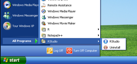
- Download RStudio from here
- Select the installation package recommended for your system (e.g. 'RStudio Desktop 0.93.84 - Windows XP/Vista/7')
- Click 'Run' and when prompted verify the publisher
- Use all of the defaults while installing
- Start RStudio from the Windows Start Menu
HowTo's
- Start a new script
- File->New->Rscript
Features
- Syntax highlighting - text colored according to syntax rules
- Code folding - mainly useful when writing functions
- Supports huge range of languages (not just R)
- Bracket matching
- Submit code to R line-by-line or selected lines (F8 key)
- Windows only
Installation and setup
- Download Notepad ++ from here
- Select 'Download the current version'
- Select 'Notepad++ v5.9 Installer'
- Click 'Run' and when prompted verify the publisher
- Use all of the defaults while installing
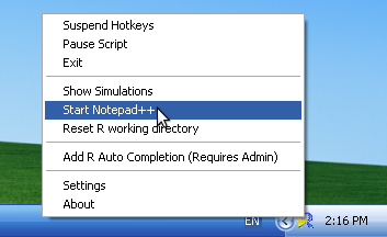
- Similarly, download and install NppToR (acts as a conduit between Notepad++ and R) from here
- Start Notepad++ (and R) by right clicking on the NppToR icon in the Windows Task Tray and selecting 'Start Notepad++'
| Feature | Notepad ++ | RStudio | Emacs |
|---|---|---|---|
| Platform | Win only | Win,Mac,Linux | Win,Mac,Linux |
| Syntax Highlighting | Yes | Yes | Yes |
| Bracket matching | Yes | Yes | |
| Integrated Console | No | Yes | Yes |
| Auto-complete | Yes | Yes | Yes |
| Parameter prompting and integrated help | No | Yes | Yes (with effort) |
| Code folding | Yes | No | Yes |
Worked examples
- Complete the following table, by
assigning the following entries
(numbers etc) to the corresponding object names and determining the
object class
for each.
Name Entry Syntax Class A 100 hint B Big hint VAR1 100 & 105 & 110 hint VAR2 5 + 6 hint VAR3 150 to 250 hint
- Print out the contents of the vector you called 'a'. Notice that the output appears on the line under the syntax that you entered, and that the output is proceeded by a [1]. This indicates that the value returned (100) is the first entry in the vector
- Print out the contents of the vector called 'b'. Again notice that the output is proceeded by [1].
- Print out the contents of the vector called 'var1'.
- Print out the contents of the vector called 'var2'. Notice that the output contains the product of the statement rather than the statement itself.
- Print out the contents of the vector called 'var3'. Notice that the output contains 100 entries (150 to 250) and that it spans multiple lines on the screen. Each new line begins with a number in square brackets [] to indicate the index of the entry that immediately follows.
- Generate the following numeric vectors (variables)
- The numbers 1, 4, 7 & 9 (call the object y)
- The numbers 10 to 25 (call the object y1)
- The sequency of numbers 2, 4, 6, 8...20 (call the object y2)
- The numbers 1, 4, 7 & 9 (call the object y)
- Generate the following character vectors (factorial/categorical variables)
- A factor that lists the sex of individuals as 6 females followed by 6 males
- A factor called TEMPERATURE that lists 10 cases of 'High', 10 'Medium & 10 'Low'
- A factor called TEMPERATURE that lists 'High', 'Medium & 'Low' alternating 10 times
- A factor called TEMPERATURE that lists 10 cases of 'High', 8 cases of 'Medium' and 11 cases of 'Low'
- A factor that lists the sex of individuals as 6 females followed by 6 males
- Print out the contents of the 'TEMPERATURE' factor. A list of factor levels will be printed on the screen. This will take up multiple lines, each of which will start with a number in square brackets [ ] to indicate the index number of the entry immediately to the right. At the end, the output also indicates what the names of the factor levels are. These are listed in alphebetical order.