Tutorial 14.2 - Principle Components Analysis (PCA)
10 Jun 2015
> library(vegan)
> library(ggplot2)
> library(grid)
> #define my common ggplot options
> murray_opts <- opts(panel.grid.major=theme_blank(),
+                            panel.grid.minor=theme_blank(),
+                            panel.border = theme_blank(),
+                            panel.background = theme_blank(),
+                            axis.title.y=theme_text(size=15, vjust=0,angle=90),
+                            axis.text.y=theme_text(size=12),
+                            axis.title.x=theme_text(size=15, vjust=-1),
+                            axis.text.x=theme_text(size=12),
+                            axis.line = theme_segment(),
+                            plot.margin=unit(c(0.5,0.5,1,2),"lines")
+ )
Error: Use 'theme' instead. (Defunct; last used in version 0.9.1)
> coenocline <- function(x,A0,m,r,a,g, int=T, noise=T) {
+ #x is the environmental range
+ #A0 is the maximum abundance of the species at the optimum environmental conditions
+ #m is the value of the environmental gradient that represents the optimum conditions for the species
+ #r the species range over the environmental gradient (niche width)
+ #a and g are shape parameters representing the skewness and kurtosis
+ # when a=g, the distribution is symmetrical
+ # when a>g - negative skew (large left tail)
+ # when a<g - positive skew (large right tail)
+ #int - indicates whether the responses should be rounded to integers (=T)
+ #noise - indicates whether or not random noise should be added (reflecting random sampling)
+ #NOTE.  negative numbers converted to 0
+          b <- a/(a+g)
+          d <- (b^a)*(1-b)^g
+          cc <- (A0/d)*((((x-m)/r)+b)^a)*((1-(((x-m)/r)+b))^g)
+          if (noise) {n <- A0/10; n[n<0]<-0; cc<-cc+rnorm(length(cc),0,n)}
+          cc[cc<0] <- 0
+          cc[is.na(cc)]<-0
+          if (int) cc<-round(cc,0)
+          cc
+ }
> #plot(coenocline(0:100,40,40,20,1,1, int=T, noise=T), ylim=c(0,100))
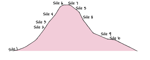
To assist with demonstrating Principle Components Analysis (PCA), we will return to the fabricated species abundance data introduced in Tutorial 13.2. This data set comprises the abundances of 10 species within 10 sites located along a transect that extends in a northerly direction over a mountain range.
> set.seed(1)
> x <- seq(0,50,l=10)
> n <- 10
> sp1<-coenocline(x=x,A0=5,m=0,r=2,a=1,g=1,int=T, noise=T)
> sp2<-coenocline(x=x,A0=70,m=7,r=30,a=1,g=1,int=T, noise=T)
> sp3<-coenocline(x=x,A0=50,m=15,r=30,a=1,g=1,int=T, noise=T)
> sp4<-coenocline(x=x,A0=7,m=25,r=20,a=0.4,g=0.1,int=T, noise=T)
> sp5<-coenocline(x=x,A0=40,m=30,r=30,a=0.6,g=0.5,int=T, noise=T)
> sp6<-coenocline(x=x,A0=15,m=35,r=15,a=0.2,g=0.3,int=T, noise=T)
> sp7<-coenocline(x=x,A0=20,m=45,r=25,a=0.5,g=0.9,int=T, noise=T)
> sp8<-coenocline(x=x,A0=5,m=45,r=5,a=1,g=1,int=T, noise=T)
> sp9<-coenocline(x=x,A0=20,m=45,r=15,a=1,g=1,int=T, noise=T)
> sp10<-coenocline(x=x,A0=30,m=50,r=5,a=1,g=1,int=T, noise=T)
> X <- cbind(sp1, sp10,sp9,sp2,sp3,sp8,sp4,sp5,sp7,sp6)
> #X<-X[c(1,10,9,2,3,8,4,5,7,6),]
> colnames(X) <- paste("Sp",1:10,sep="")
> rownames(X) <- paste("Site", c(1,10,9,2,3,8,4,5,7,6), sep="")
> X <- X[c(1,4,5,7,8,10,9,6,3,2),]
> data <- data.frame(Sites=factor(rownames(X),levels=rownames(X)), X)
| Sites | Sp1 | Sp2 | Sp3 | Sp4 | Sp5 | Sp6 | Sp7 | Sp8 | Sp9 | Sp10 |
|---|---|---|---|---|---|---|---|---|---|---|
| Site1 | 5 | 0 | 0 | 65 | 5 | 0 | 0 | 0 | 0 | 0 |
| Site2 | 0 | 0 | 0 | 25 | 39 | 0 | 6 | 23 | 0 | 0 |
| Site3 | 0 | 0 | 0 | 6 | 42 | 0 | 6 | 31 | 0 | 0 |
| Site4 | 0 | 0 | 0 | 0 | 0 | 0 | 0 | 40 | 0 | 14 |
| Site5 | 0 | 0 | 6 | 0 | 0 | 0 | 0 | 34 | 18 | 12 |
| Site6 | 0 | 29 | 12 | 0 | 0 | 0 | 0 | 0 | 22 | 0 |
| Site7 | 0 | 0 | 21 | 0 | 0 | 5 | 0 | 0 | 20 | 0 |
| Site8 | 0 | 0 | 0 | 0 | 13 | 0 | 6 | 37 | 0 | 0 |
| Site9 | 0 | 0 | 0 | 60 | 47 | 0 | 4 | 0 | 0 | 0 |
| Site10 | 0 | 0 | 0 | 72 | 34 | 0 | 0 | 0 | 0 | 0 |
Principal components analysis (PCA)
Principle components analysis (PCA) can be performed by either spectral (eigen) decomposition of an association matrix or single value decomposition of the original data matrix. Either way, it yields a rigid rotation of axes in that the positions of points relative to one another (euclidean distances) are maintained during rotation. The rotated axes are referred to as principle components.
Obviously, the higher the degree of associations between the variables (species), the more strongly focused and oriented the data cloud is and therefore the more 'successful' the PCA in terms of being able to represent many variables by only a few new variables.
The resulting principle components (axes) and scores (new variable values) are independent of one another and therefore the 'reduced data' can be used in subsequent statistical analyses. For example, principle component 1 (as one measure of the community) could be regressed against an environmental variable (such as altitude or rainfall) in a regular linear modelling procedure. Similarly, multiple correlated predictor variables (that otherwise violate multi-collinearity) could be reduced to one or two orthogonal predictors to use in linear modelling. Principle components analysis is therefore often an intermediate step to used as either responses or predictors in linear modeling.
In PCA, the sum of the eigenvalues will be equal to the sum of the variances of the association matrix.
- if the association matrix is a variance-covariance matrix, then the sum of the eigenvalues will be equal to the sum of the variances of all variables (species).
- if the association matrix is a correlation matrix, then the sum of the eigenvalues will be equal to the number of variables (species).
In R, PCA via spectral decomposition is implemented in the princomp() function and via either prcomp() or rda() (from the vegan package). We will first explore the simpler spectral decomposition route (using the princomp() function).
princomp()
Lets perform a principle components analysis on the species abundance data. We will indicate that a correlation matrix should be used as the association matrix (cor=T). This is equivalent to centering and scaling the data and thus each variable has equal influence (rare taxa are promoted at the expense of very abundant taxa). Since axes rotation orients axes on the basis of greatest variance in data, the axes will tend to orient towards variables that are substantially more variable than other variables (larger magnitudes of values). If the variances of the variables are substantially different from one another, then it is advisable that correlations be used.
> data.pca <- princomp(data[,-1], cor=TRUE)
> summary(data.pca, loadings=TRUE)
Importance of components:
                         Comp.1
Standard deviation     1.955001
Proportion of Variance 0.382203
Cumulative Proportion  0.382203
                          Comp.2
Standard deviation     1.5557921
Proportion of Variance 0.2420489
Cumulative Proportion  0.6242519
                          Comp.3
Standard deviation     1.2943370
Proportion of Variance 0.1675308
Cumulative Proportion  0.7917827
                          Comp.4
Standard deviation     1.0817301
Proportion of Variance 0.1170140
Cumulative Proportion  0.9087967
                           Comp.5
Standard deviation     0.81775539
Proportion of Variance 0.06687239
Cumulative Proportion  0.97566911
                           Comp.6
Standard deviation     0.38265939
Proportion of Variance 0.01464282
Cumulative Proportion  0.99031193
                            Comp.7
Standard deviation     0.260454350
Proportion of Variance 0.006783647
Cumulative Proportion  0.997095576
                            Comp.8
Standard deviation     0.167331033
Proportion of Variance 0.002799967
Cumulative Proportion  0.999895544
                             Comp.9
Standard deviation     0.0323196987
Proportion of Variance 0.0001044563
Cumulative Proportion  1.0000000000
                       Comp.10
Standard deviation           0
Proportion of Variance       0
Cumulative Proportion        1

Loadings:
     Comp.1 Comp.2 Comp.3 Comp.4 Comp.5
Sp1         -0.326  0.504         0.634
Sp2  -0.263 -0.104         0.758
Sp3  -0.473 -0.113 -0.220 -0.160
Sp4   0.275 -0.471  0.221        -0.347
Sp5   0.397 -0.130 -0.381        -0.330
Sp6  -0.326 -0.141 -0.251 -0.600
Sp7   0.331  0.153 -0.486         0.402
Sp8   0.116  0.611                0.217
Sp9  -0.478                0.137
Sp10 -0.103  0.463  0.430        -0.381
     Comp.6 Comp.7 Comp.8 Comp.9
Sp1   0.301  0.342 -0.120
Sp2  -0.280  0.325         0.346
Sp3   0.102  0.108         0.236
Sp4         -0.289  0.246  0.617
Sp5   0.344  0.511 -0.435
Sp6  -0.271  0.260         0.254
Sp7   0.230         0.632  0.115
Sp8         -0.186 -0.415  0.595
Sp9   0.735 -0.272
Sp10  0.172  0.492  0.401
     Comp.10
Sp1
Sp2  -0.160
Sp3   0.782
Sp4
Sp5
Sp6  -0.491
Sp7
Sp8
Sp9  -0.350
Sp10
The summary of the analysis displays the eigenvalues (in units of standard deviation). These are also expressed as a
percentage and cumulative percentage.
The first principle component explains 38.22%
of the variation.
The loadings (eigenvectors) indicate the degree of correlation between the original variables and the new principle components. In this way they indicate how much each of the original variables contribute to the new variables. In this example it is clear that principle component 1 is made up of fairly uniform contributions from all of the original variables (except perhaps species 1 and 3). Given the strength of this principle component, the underlying gradient it represents appears to have an influence on many aspects of the community.
The sign of an eigenvector indicates the polarity of the correlation between the original variable and the new variable.
Species 1 and 3 seem to be the major contributors to principle component 2. Perhaps this represents another environmental gradient that species 1 and 3 are more sensitive to than the others. Many of the remaining principle components (that did not explain much of the original variation) have few major contributors and thus probably represent the unique responses of individual characteristics (species). Blank eigenvector values are just considered too small to warrant display.
Axes retention
Recall that one of the goals of R-mode analyses is to reduce a large number of variables that characterize a community to a smaller number of independent variables that can be used in subsequent analyses. In our example, we started with three variables (abundances of three species) and ended up with three new dimensions representing the same data (from another perspective). So what have we really achieved.
Consider again what each of the new variables (dimensions) represent. The first principle component is orientated through the data cloud in the direction of the greatest spread (trend). The next principle component is orientated in the direction of the greatest spread remaining and so on. If there are correlations between the original variables, then the latter principle components will probably just represent noise. It is only the first few principle components that are likely to represent real trends.
Consequently, we can just keep those principle components (axes) that explain that capture substantial amounts of the original variability. Recall that the eigenvalues (also called latent roots) quantify how much of the original variability is explained by each of the principle components. There are three bases on which to use these eigenvalues for determining how many principle components to retain.
- Retain axes (principle components) such that the cumulative proportions explained by the axes just exceeds 80%.
In this case we would retain the first three principle components ( which explain
79.18%). - Since the sum of the eigenvalues (in variance units) is equal to the number of original variables, purely random
axes rotations should yield eigenvalues of approximately 1 for each principle component. Therefore eigenvalues greater than
one indicate that the new axis is explaining more than its share of the original variance. Conversely, eigenvalues less than
one correspond to variables that explain less than their share.
Hence, we could elect to retain only those principle components whose eigenvalues are greater than 1.
By this rule, we would again retain the first three principle components.> round(data.pca$sdev^2,2)
 Comp.1  Comp.2  Comp.3  Comp.4  Comp.5
   3.82    2.42    1.68    1.17    0.67
 Comp.6  Comp.7  Comp.8  Comp.9 Comp.10
   0.15    0.07    0.03    0.00    0.00
- There are often a relatively large number of principle components with eigenvalues greater than one (particularly when there
were a large number of original variables). When this case, it is often better to plot the eigenvalues as a histogram.
This is known as a screeplot. Major elbows (or kinks, changes in direction) in the screeplot indicate
points at which the relative value of additional components changes. So a general rule is to keep all components up to the elbow.
The screeplot can be produced using the screeplot function.
In this example, there are two possible elbows. One between components 1 and 2 and another between components 3 and 4. We could therefore justify capping the number of principle components at either 1 or 3.
> screeplot(data.pca)

Ordination plot
An ordination plot, plots the objects (sites) in the reduced dimensional space. That is, it displays the objects in one, two or three dimensions so that the major patterns amongst objects can be visualized.
The new coordinates are calculated by using the eigenvectors (component loadings) as the weightings in the linear model with scaled versions of the original vectors ($y$): $$\textbf{X} = c_0 + c_{1}y_{i1}+c_2y_{i2}+...+c_jy_{ij}$$ and are often called the axes scores and are stored in the pca object as scores. The centers and standard deviations of the scaled original data are also stored in the pca object.
> scale(data[,-1], center = data.pca$center, scale = data.pca$scale) %*% data.pca$loadings
           Comp.1     Comp.2     Comp.3
Site1   0.7825501 -2.3688257  2.5335395
Site2   1.7685536  0.2935564 -1.1400547
Site3   1.7063613  0.8679611 -1.3260717
Site4  -0.1676240  2.4848095  1.7046156
Site5  -1.5186651  1.9803978  1.1437051
Site6  -3.0108352 -0.7536609 -0.4664866
Site7  -3.7408656 -1.0250009 -1.2639273
Site8   1.0837586  1.3788118 -0.7766807
Site9   1.8687783 -1.2650232 -0.7336800
Site10  1.2279879 -1.5930259  0.3250410
              Comp.4     Comp.5
Site1  -2.969091e-01  1.2722736
Site2   2.770594e-02  0.2150604
Site3   3.184052e-02  0.4916520
Site4  -2.688294e-01 -0.4912986
Site5  -8.875218e-02 -0.5357291
Site6   2.662100e+00  0.1597642
Site7  -2.107679e+00  0.1016205
Site8  -6.553076e-05  1.1446501
Site9   4.681628e-02 -0.9279340
Site10 -6.227973e-03 -1.4300592
           Comp.6      Comp.7
Site1   0.1321870  0.06950862
Site2   0.1720803  0.10477437
Site3   0.1873296  0.28686390
Site4  -0.6207592  0.32494247
Site5   0.8335420 -0.23387595
Site6  -0.1230187  0.06607664
Site7  -0.1191365  0.05299591
Site8  -0.3462617 -0.49995276
Site9   0.2122245  0.18652277
Site10 -0.3281874 -0.35785598
             Comp.8        Comp.9
Site1  -0.010045342  0.0001973846
Site2   0.087323584  0.0834325305
Site3  -0.337752893 -0.0321254475
Site4   0.050817451  0.0021247970
Site5  -0.010482988 -0.0021335938
Site6   0.002766586  0.0010845153
Site7   0.002268968  0.0007950366
Site8   0.129923630 -0.0224286601
Site9   0.302379120 -0.0424898856
Site10 -0.217198116  0.0115433231
             Comp.10
Site1  -2.101546e-18
Site2   1.968544e-15
Site3  -2.638881e-15
Site4   7.906407e-16
Site5  -5.240281e-16
Site6  -6.959909e-16
Site7  -6.959909e-16
Site8   5.252544e-16
Site9   2.329367e-15
Site10 -1.778458e-15
> #OR
> data.pca$scores
           Comp.1     Comp.2     Comp.3
Site1   0.7825501 -2.3688257  2.5335395
Site2   1.7685536  0.2935564 -1.1400547
Site3   1.7063613  0.8679611 -1.3260717
Site4  -0.1676240  2.4848095  1.7046156
Site5  -1.5186651  1.9803978  1.1437051
Site6  -3.0108352 -0.7536609 -0.4664866
Site7  -3.7408656 -1.0250009 -1.2639273
Site8   1.0837586  1.3788118 -0.7766807
Site9   1.8687783 -1.2650232 -0.7336800
Site10  1.2279879 -1.5930259  0.3250410
              Comp.4     Comp.5
Site1  -2.969091e-01  1.2722736
Site2   2.770594e-02  0.2150604
Site3   3.184052e-02  0.4916520
Site4  -2.688294e-01 -0.4912986
Site5  -8.875218e-02 -0.5357291
Site6   2.662100e+00  0.1597642
Site7  -2.107679e+00  0.1016205
Site8  -6.553076e-05  1.1446501
Site9   4.681628e-02 -0.9279340
Site10 -6.227973e-03 -1.4300592
           Comp.6      Comp.7
Site1   0.1321870  0.06950862
Site2   0.1720803  0.10477437
Site3   0.1873296  0.28686390
Site4  -0.6207592  0.32494247
Site5   0.8335420 -0.23387595
Site6  -0.1230187  0.06607664
Site7  -0.1191365  0.05299591
Site8  -0.3462617 -0.49995276
Site9   0.2122245  0.18652277
Site10 -0.3281874 -0.35785598
             Comp.8        Comp.9
Site1  -0.010045342  0.0001973846
Site2   0.087323584  0.0834325305
Site3  -0.337752893 -0.0321254475
Site4   0.050817451  0.0021247970
Site5  -0.010482988 -0.0021335938
Site6   0.002766586  0.0010845153
Site7   0.002268968  0.0007950366
Site8   0.129923630 -0.0224286601
Site9   0.302379120 -0.0424898856
Site10 -0.217198116  0.0115433231
             Comp.10
Site1  -2.101546e-18
Site2   1.968544e-15
Site3  -2.638881e-15
Site4   7.906407e-16
Site5  -5.240281e-16
Site6  -6.959909e-16
Site7  -6.959909e-16
Site8   5.252544e-16
Site9   2.329367e-15
Site10 -1.778458e-15
A simple ordination plot can be produced by plotting the scores of one principle component against another using the base graphics techniques demonstrated in Tutorial 5. Using object names (site names) helps for identifying the objects in the plot.
> plot(data.pca$scores[,1],data.pca$scores[,2], type="n")
> # the site names are in the first column
> text(data.pca$scores[,1],data.pca$scores[,2],data[,1])

With a bit of tweaking with either base graphics or ggplot2 we can establish a really nice looking ordination plot.
 |
|
> par(mar = c(4, 5, 1, 1), xpd = T)
> plot(data.pca$scores[, 1], data.pca$scores[,
+     2], type = "n", axes = FALSE, ann = FALSE)
> # the site names are in the first column
> text(data.pca$scores[, 1], data.pca$scores[,
+     2], data[, 1])
> axis(1)
> mtext("Principle component 1", 1, line = 3)
> axis(2)
> mtext("Principle component 2", 2, line = 3)
> box(bty = "l")
> dt <- data.frame(Sites=data[,1],data.pca$scores[,1:2]) > library(ggplot2) > p <- ggplot(dt, aes(x=Comp.1, y=Comp.2)) + geom_text(aes(label=Sites))+ + scale_y_continuous("Principle component 2")+scale_x_continuous("Principle component 1")+ + murray_opts > p |
|
Biplot
The ordination plot allows us to visualize how alike the objects (sites) are to one another. We can add to this by overlaying the eigenvectors associated with each of the principle components featured on the ordination plot. Rather than plot the eigenvector coordinates as points (and them getting lost amongst the site points), they are typically represented by arrows. The arrows originate at the origin (0,0) and extend out to the eigenvector values for each principle component. Moreover, arrows give the sense of vectors - as in Variable one tends to align showing which axis each variable aligns to.
Such a plot that has both the objects as points and the variables as arrows is known as a biplot. In R, the biplot() function provides a simple biplot.
> biplot(data.pca)

The arrow lengths are generally scaled to fit within the bounds of the limits defined by the axes scores and they provide a relative indication of the strength and polarity of the associations.
In the example, it is clear that most of the variables (species) align predominantly with principle component 1. Species 3 aligns mostly with principle component 2 and Species 1 is aligns with both (although slightly more with principle component 2).
rda()
In contrast to spectral (eigen) decomposition based PCA, single value decomposition PCA starts with the rectangular data matrix. Although this makes it more difficult to conceptualize, it is more numerically stable. Whilst we can perform single value decomposition via either prcomp() or rda(), the later (from the vegan package) is more versatile and captures a richer array of information. As a result, we will focus on the rda() function.
The rda() is used for PCA (as will be demonstrated here) as well as constrained PCA (Redundancy analysis or RDA, hence the function name). As a result, some of the information captured by the rda object will not be meaningful in the context of PCA.
The influence of abundant species is dampened by scaling to unit variance (variance of 1) which is analogous to using a correlation matrix.
> library(vegan)
> data.rda <- rda(data[,-1], scale=TRUE)
> summary(data.rda, scaling=2)
Call:
rda(X = data[, -1], scale = TRUE)

Partitioning of correlations:
              Inertia Proportion
Total              10          1
Unconstrained      10          1

Eigenvalues, and their contribution to the correlations

Importance of components:
                         PC1    PC2
Eigenvalue            3.8220 2.4205
Proportion Explained  0.3822 0.2420
Cumulative Proportion 0.3822 0.6242
                         PC3    PC4
Eigenvalue            1.6753 1.1701
Proportion Explained  0.1675 0.1170
Cumulative Proportion 0.7918 0.9088
                          PC5     PC6
Eigenvalue            0.66872 0.14643
Proportion Explained  0.06687 0.01464
Cumulative Proportion 0.97567 0.99031
                          PC7    PC8
Eigenvalue            0.06784 0.0280
Proportion Explained  0.00678 0.0028
Cumulative Proportion 0.99710 0.9999
                           PC9
Eigenvalue            0.001045
Proportion Explained  0.000100
Cumulative Proportion 1.000000

Scaling 2 for species and site scores
* Species are scaled proportional to eigenvalues
* Sites are unscaled: weighted dispersion equal on all dimensions
* General scaling constant of scores:  3.08007


Species scores

         PC1       PC2      PC3
Sp1  -0.1300 -0.494334 -0.63551
Sp2   0.5000 -0.157276  0.11701
Sp3   0.9007 -0.170843  0.27779
Sp4  -0.5235 -0.714165 -0.27820
Sp5  -0.7564 -0.196662  0.47970
Sp6   0.6212 -0.213901  0.31704
Sp7  -0.6311  0.231834  0.61283
Sp8  -0.2207  0.925419 -0.04869
Sp9   0.9110 -0.009745  0.12221
Sp10  0.1964  0.702341 -0.54197
          PC4      PC5       PC6
Sp1   0.08911 -0.50512  0.112154
Sp2  -0.79900 -0.06343 -0.104375
Sp3   0.16895 -0.01456  0.038032
Sp4   0.04967  0.27670  0.027303
Sp5  -0.01385  0.26323  0.128107
Sp6   0.63259 -0.04035 -0.101082
Sp7  -0.01782 -0.32040  0.085889
Sp8   0.06432 -0.17279  0.006936
Sp9  -0.14486  0.05298  0.274048
Sp10  0.08330  0.30368  0.063979


Site scores (weighted sums of species scores)

            PC1     PC2     PC3
Site1  -0.38988 -1.4830 -1.9065
Site2  -0.88111  0.1838  0.8579
Site3  -0.85013  0.5434  0.9979
Site4   0.08351  1.5556 -1.2827
Site5   0.75662  1.2398 -0.8607
Site6   1.50003 -0.4718  0.3510
Site7   1.86374 -0.6417  0.9511
Site8  -0.53994  0.8632  0.5845
Site9  -0.93105 -0.7920  0.5521
Site10 -0.61180 -0.9973 -0.2446
             PC4     PC5     PC6
Site1   0.267341 -1.5154  0.3365
Site2  -0.024947 -0.2562  0.4380
Site3  -0.028670 -0.5856  0.4768
Site4   0.242057  0.5852 -1.5801
Site5   0.079914  0.6381  2.1217
Site6  -2.396989 -0.1903 -0.3131
Site7   1.897781 -0.1210 -0.3032
Site8   0.000059 -1.3634 -0.8814
Site9  -0.042154  1.1052  0.5402
Site10  0.005608  1.7033 -0.8354
Lets go through the output
- Partitioning of correlations reflects the scale=TRUE parameter.
- inertia is a term used to refer to the sum of the variables (covariance matrix) or correlation matrix diagonals (scale=TRUE). In the later case (which is the case here), inertia equates to the number of variables.
- eigenvalues are the amount of variance explained by each of the new principle components and thus a measure of importance
of each principle component. When a correlation matrix is applied, then the eigenvalues will sum up to the number of variables.
These are also expressed as percentage and cumulative percentage of their sums.
Note, that the eigenvalues are in units of variance and that to save space, the output does not include all eigenvalues (only the most important ones).
In this case, principle component 1 explains
38.22%of the variance. - scaling refers to the way either objects (sites) or variables (species) are scaled so that they can both be sensibly included on
a biplot.
- (scaling=1) the eigenvectors (site scores) are scaled to be proportional to the eigenvalues. This is a good option if the main focus is to interpret the relationships amongst objects (sites).
- (scaling=2) the eigenvectors (site scores) are scaled to the square-root of the eigenvalues. This is a good option if the main focus is to interpret the relationships amongst variables (species).
- species scores these are the (scaled) eigenvectors (loadings) that represent the degree of correlation between each of the original variables and the new principle components.
- site scores these are the (scaled) coordinates of the objects (sites).
Axis retention
Determining the number of axes (principle components) to retain follows the same 'rules' outlined in above.
> #the eigenvalues
> data.rda$CA$eig
        PC1         PC2         PC3
3.822030054 2.420488947 1.675308207
        PC4         PC5         PC6
1.170140005 0.668723871 0.146428210
        PC7         PC8         PC9
0.067836468 0.027999675 0.001044563
> #expressed as cumulative percentages
> round(cumsum(100*data.rda$CA$eig/sum(data.rda$CA$eig)),2)
   PC1    PC2    PC3    PC4    PC5
 38.22  62.43  79.18  90.88  97.57
   PC6    PC7    PC8    PC9
 99.03  99.71  99.99 100.00
> #screeplot
> screeplot(data.rda)
> abline(a=1,b=0)

- Again, we could justify retaining either just the first principle component or else the first three principle components.
Biplot
Again, there is a convenience function called biplot() that can be used to produce simple biplots. When the main focus is on the relationships between variables (species), a scaling specifier of 2 is most sensible. When doing so, it is also useful to include a circle of equilibrium contribution. This circle (the radius of which is equal to the square-root of the ratio of plot dimensions to number of variables) defines a region beyond which variables (species) can be interpreted with greatest confidence.
 |
 |
> biplot(data.rda, scaling = 1, main = "Scaling=1") > biplot(data.rda, scaling=2, main="Scaling=2") > d <- 2 > p <- 10 > cec <- sqrt(d/p) > > circ <- seq(0,2*pi,length=100) > coords <- t(rbind(sin(circ)*cec, cos(circ)*cec)) > lines(coords, col="blue") |
|
Using the principle components in subsequent analysis
If major patterns existed between the variables, then the PCA should be able to reduce the variables down to a smaller number that hopefully contain the bulk of the original variability. The resulting retained principle components should reflect the major underling environmental gradients.
For example, close inspection of the arrangement of sites along principle component 1 (x-axis) does suggest that there is a hint of a altitude effect (sites on the left hand side of the ordination were typically sampled from lower on the mountain range).
Since each of the principle components are independent of one another, as are their scores, we can use these principle components as responses to simple or multiple regressions against the environmental variables to explore the assocations more formally.
Lets first retrieve the environmental variables collected from the 10 sites.
> set.seed(1)
> Site <- gl(10,1,10,lab=paste('Site',1:10, sep=""))
>
> Y <- matrix(c(
+ 6.1,4.2,101325,2,
+ 6.7,9.2,101352,510,
+ 6.8,8.6,101356,546,
+ 7.0,7.4,101372,758,
+ 7.2,5.8,101384,813,
+ 7.5,8.4,101395,856,
+ 7.5,0.5,101396,854,
+ 7.0,11.8,101370,734,
+ 8.4,8.2,101347,360,
+ 6.2,1.5,101345,356
+   ),10,4, byrow=TRUE)
> colnames(Y) <- c('pH','Slope', 'Pressure', 'Altitude')
> Substrate <- factor(c('Quartz','Shale','Shale','Shale','Shale','Quartz','Quartz','Shale','Quartz','Quartz'))
> enviro <- data.frame(Site,Y,Substrate)
As always, prior to leaping in and fitting a model, we should explore the data to gain an appreciation of the suitability and compatibility of the data and model. Lets start by producing some scatterplot matrices to explore the nature of relationships between the principle components and the predictors.
> #PC1
> pairs(cbind(data.rda$CA$u[,1],enviro[,-1]))

> #PC2
> pairs(cbind(data.rda$CA$u[,2],enviro[,-1]))

> #PC3
> pairs(cbind(data.rda$CA$u[,3],enviro[,-1]))

- Altitude and pressure are very highly correlated predictors (not surprisingly) and should not be used in the same model
- There is no major evidence of non-normality between the responses (PC's) and the predictors - although the relationship between PC1 and ALtitude is perhaps slightly curved.
Now lets regress the first three principle components (individually) against a couple of these environmental predictions (altitude, temperature and slope).
> #we should also confirm variance inflations are ok (each should be less than 5)
> library(car)
> vif(lm(data.rda$CA$u[,1]~Slope+Altitude+Substrate+pH, data=enviro))
    Slope  Altitude Substrate        pH
 2.116732  1.830014  2.636302  1.968157
> #specify linear models relating each of the first three principle components against
> # a linear predictor comprising Slope, Altitude, Substrate and pH
> data.lm <- lm(data.rda$CA$u[,1:3] ~ enviro$Slope + enviro$Altitude + enviro$Substrate+enviro$pH)
> # summarize the models
> summary(data.lm)
Response PC1 :

Call:
lm(formula = PC1 ~ enviro$Slope + enviro$Altitude + enviro$Substrate +
    enviro$pH)

Residuals:
    Site1     Site2     Site3     Site4
 0.239795 -0.014671 -0.050466  0.003064
    Site5     Site6     Site7     Site8
 0.140531  0.085398  0.037275 -0.078458
    Site9    Site10
-0.080953 -0.281515

Coefficients:
                        Estimate
(Intercept)            0.1807875
enviro$Slope          -0.0213244
enviro$Altitude        0.0011277
enviro$SubstrateShale -0.3260633
enviro$pH             -0.0753861
                      Std. Error
(Intercept)            0.8121648
enviro$Slope           0.0259196
enviro$Altitude        0.0003074
enviro$SubstrateShale  0.1951991
enviro$pH              0.1322828
                      t value Pr(>|t|)
(Intercept)             0.223   0.8327
enviro$Slope           -0.823   0.4481
enviro$Altitude         3.668   0.0145
enviro$SubstrateShale  -1.670   0.1557
enviro$pH              -0.570   0.5934

(Intercept)
enviro$Slope
enviro$Altitude       *
enviro$SubstrateShale
enviro$pH
---
Signif. codes:
  0 '***' 0.001 '**' 0.01 '*' 0.05
  '.' 0.1 ' ' 1

Residual standard error: 0.1901 on 5 degrees of freedom
Multiple R-squared:  0.8193,	Adjusted R-squared:  0.6748
F-statistic: 5.669 on 4 and 5 DF,  p-value: 0.04229


Response PC2 :

Call:
lm(formula = PC2 ~ enviro$Slope + enviro$Altitude + enviro$Substrate +
    enviro$pH)

Residuals:
    Site1     Site2     Site3     Site4
 0.025466 -0.151353 -0.057143  0.179078
    Site5     Site6     Site7     Site8
 0.034234  0.013755 -0.099604 -0.004816
    Site9    Site10
 0.022940  0.037443

Coefficients:
                        Estimate
(Intercept)           -0.8361051
enviro$Slope          -0.0074536
enviro$Altitude        0.0003381
enviro$SubstrateShale  0.5480945
enviro$pH              0.0589811
                      Std. Error
(Intercept)            0.5131551
enviro$Slope           0.0163769
enviro$Altitude        0.0001942
enviro$SubstrateShale  0.1233339
enviro$pH              0.0835811
                      t value Pr(>|t|)
(Intercept)            -1.629  0.16417
enviro$Slope           -0.455  0.66810
enviro$Altitude         1.741  0.14223
enviro$SubstrateShale   4.444  0.00674
enviro$pH               0.706  0.51190

(Intercept)
enviro$Slope
enviro$Altitude
enviro$SubstrateShale **
enviro$pH
---
Signif. codes:
  0 '***' 0.001 '**' 0.01 '*' 0.05
  '.' 0.1 ' ' 1

Residual standard error: 0.1201 on 5 degrees of freedom
Multiple R-squared:  0.9279,	Adjusted R-squared:  0.8702
F-statistic: 16.08 on 4 and 5 DF,  p-value: 0.004638


Response PC3 :

Call:
lm(formula = PC3 ~ enviro$Slope + enviro$Altitude + enviro$Substrate +
    enviro$pH)

Residuals:
   Site1    Site2    Site3    Site4
-0.30906  0.32692  0.36225 -0.44520
   Site5    Site6    Site7    Site8
-0.31368 -0.11906  0.25477  0.06971
   Site9   Site10
 0.01179  0.16156

Coefficients:
                        Estimate
(Intercept)           -1.1148133
enviro$Slope           0.0225742
enviro$Altitude        0.0003341
enviro$SubstrateShale -0.0908323
enviro$pH              0.1162957
                      Std. Error
(Intercept)            1.6441465
enviro$Slope           0.0524716
enviro$Altitude        0.0006224
enviro$SubstrateShale  0.3951612
enviro$pH              0.2677933
                      t value Pr(>|t|)
(Intercept)            -0.678    0.528
enviro$Slope            0.430    0.685
enviro$Altitude         0.537    0.614
enviro$SubstrateShale  -0.230    0.827
enviro$pH               0.434    0.682

Residual standard error: 0.3848 on 5 degrees of freedom
Multiple R-squared:  0.2596,	Adjusted R-squared:  -0.3327
F-statistic: 0.4383 on 4 and 5 DF,  p-value: 0.7778
- An increase in Altitude is associated with a significant positive increase in PC1
- The community composition (as measured by PC2) was found to differ according to substrate. Shale substrates had significantly larger PC2 values (sites dominated by Species 7, 8 and 10) than quartz sites.
- PC3 was not found to be associated with any of the measured environmental variables
Additional considerations of PCA
In addition to species abundance data, PCA can handle environmental data involving measurements. Indeed, as it is essentially based on euclidean distances, PCA can accommodate any positive or negative numbers and the ability to center and scale in a way that dampens the influence of highly variable and large magnitude variables makes it particularly suitable for environmental variables.
PCA does not perform well variables are not linearly related and performs even worse when unimodal relationships exist. Recall a unimodal relationship is one that has a major alteration in direction (such as a parabola). Unfortunately, most species abundance data is unimodal.
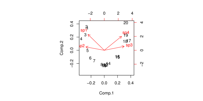
Consider another fabricated data set that depicts the abundance of four species from a total of 20 sites sampled evenly across an unknown (yet very broad) environmental gradient. The environmental gradient is sufficiently wide as to transcend entire communities.
> set.seed(2)
> ENV <- seq(0,30,l=20)
> sp1 <- round(150*dnorm(ENV,1,3),0)
> sp1<-sp1+rpois(20,sp1)
> sp2 <- round(100*dnorm(ENV,6,3),0)
> sp2<-sp2+rpois(20,sp2)
> sp3 <- round(100*dnorm(ENV,25,3),0)
> sp3<-sp3+rpois(20,sp3)
> sp4 <- round(150*dnorm(ENV,30,3),0)
> sp4<-sp4+rpois(20,sp4)
> #sp4 <- round(100*dnorm(ENV,20,3),0)+rnorm(20,0,0.5)
> data1 <- data.frame(sp1,sp2,sp3,sp4)
> #par(mfrow=c(2,1))
> #biplot(princomp(data1, cor=T))
> #plot(sp1~ENV,type="l");lines(sp2~ENV);lines(sp3~ENV);lines(sp4~ENV)
> #pairs(data1)
If we plot the abundances of each species against this environmental gradient, it is clear that there is almost no overlap between the community comprising species 1 and 2 and the community of species 3 and 4.
Note also that the abundances of species 2 and 3 across the environmental gradient are strongly curvilinear (actually unimodal). A unimodal species distribution increases up to a peak (representing optimal conditions) before declining again as the conditions get increasingly less favorable. The presence of such a distribution along an environmental gradient indicates that the environmental conditions span the entire niche of this species is the result of Most species. The problem is that since no two species niches are likely to overlap exactly (and they clearly do not in this example), the individual relationships between the difference species will not be linear.


Recall that the rotated axes in a PCA are linear (they are axes after all). So, analogous to linear regression, PCA attempts to fit a linear line through the major axis of variance in a data cloud. If the inter-variable relationships are non-linear, then the multivariate data cloud will also be non-linear (or the multivariate equivalent thereof). Consequently, the axes do not adequately represent the trends.
The following biplot demonstrates the consequence of performing a PCA on species abundance data sampled across a large environmental range. The pattern in known as the horseshoe effect. The horseshoe effect is characterized by the arrangement of sites in curved pattern that begins to curl in on itself towards the ends. Unfortunately, since species response curves are frequently unimodal (curvilinear), horseshoe effects are particularly vexing for ecologists.
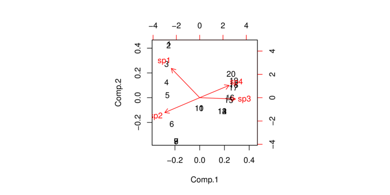
One way to deal with this issue is to perform a Hellinger transformation on the data prior to running the PCA. A Hellinger transformation is essentially a euclidean distance matrix.
> data1.hel <- decostand(data1, "hel")
> biplot(princomp(data1.hel, cor=T))
Finally, another avenue for analyzing species abundance data is Correspondence Analysis (CA).
Worked Examples
Basic statistics references
- Legendre and Legendre
- Quinn & Keough (2002) - Chpt 17
Principle components analysis
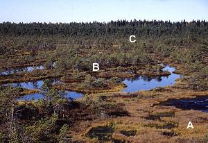
Gittens(1985) measured the abundance of 8 species of plants from 45 sites within 3 habitat types. Essentially, the plant ecologist wanted to be able to compare the sites according to their plant communities.
Download veg data set| Format of veg.csv data file | ||||||||||||||||||||||||||||||||||||||||||||||||||||||||||||||
|---|---|---|---|---|---|---|---|---|---|---|---|---|---|---|---|---|---|---|---|---|---|---|---|---|---|---|---|---|---|---|---|---|---|---|---|---|---|---|---|---|---|---|---|---|---|---|---|---|---|---|---|---|---|---|---|---|---|---|---|---|---|---|
|
 |
> veg <- read.csv('../downloads/data/veg.csv')
> veg
   SITE HABITAT SP1 SP2 SP3 SP4 SP5 SP6
1     1       A   4   0   0  36  28  24
2     2       B  92  84   0   8   0   0
3     3       A   9   0   0  52   4  40
4     4       A  52   0   0  52  12  28
5     5       C  99   0  36  88  52   8
6     6       A  12   0   0  20  40  40
7     7       C  72   0  20  72  24  20
8     8       C  80   0   0  48  16  28
9     9       B  80  76   4   8  12   0
10   10       C  92   0  40  72  36  12
11   11       A  28   4   0  16  56  28
12   12       A   8   0   0  36  68   8
13   13       C  99  12   4  84  36  12
14   14       A  40   0   0  68  12   8
15   15       A  28   0   0  36  64  28
16   16       A  28   0   0  28  44  20
17   17       C  80   0   0  52  20  32
18   18       C  84   0   0  76  44  16
19   19       B  88  40  12   8  24   8
20   20       C  99   0  60  88  28   0
21   21       A  12   0   0  36  16  12
22   22       A   0   0   0  20   8   0
23   23       C  88   0  12  72  32  16
24   24       C  56   0   4  32  56   4
25   25       C  99   0  40  60  20   4
26   26       A  12   0   0  28   4   4
27   27       A  28   0   0  48  64   4
28   28       B  92  52   0  40  64   8
29   29       C  80   0   0  68  40  12
30   30       A  32   0   0  56  28  36
31   31       A  40   0   0  60   8  36
32   32       A  44   0   0  44   8  20
33   33       A  48   0   0  72  20  12
34   34       A  48   0   0   8  44   8
35   35       B  99  36  20  56   8   4
36   36       A  15   0   4  36   4  28
37   37       A   8   0   0  20  16  12
38   38       A  28   0   0  24  16  12
39   39       A  52   0   0  48  12  28
40   40       C  92   0   4  56  12  16
41   41       C  92   0   8  52  56   8
42   42       A   4   0   0  44  24   4
43   43       A  16   0   0  36   0  24
44   44       A  76   0   0  48  12  36
45   45       B  96  36   4  28  28   8
   SP7 SP8
1   99  68
2   84   4
3   96  68
4   96  24
5   72   0
6   88  68
7   72   8
8   92   8
9   84   0
10  84   0
11  96  56
12  99  28
13  88   8
14  88  24
15  99  56
16  88  32
17  96  20
18  96   0
19  92   0
20  80   0
21  88  76
22  99  60
23  88   0
24  96  16
25  56   4
26  99  72
27  99  28
28  96   4
29  80   8
30  84  24
31  96  56
32  96  24
33  99  32
34  92  56
35  24   0
36  99  44
37  99  56
38  99  36
39  99  32
40  70   4
41  99   4
42  99  60
43  99  76
44  96  32
45  88   4
-
Before leaping into a multivariate analysis, we will begin by
treating the data set as a series of univariate responses (only a single response variable), and
examine the patterns between habitats based on the following single species:
- SP1
Show codeWhat does this plot illustrate about the relationships between habitats based on this plant species?
> plot(SP1~SITE, col=as.numeric(HABITAT),data=veg, pch=16)

- SP2
Show codeWhat does this plot illustrate about the relationships between habitats based on this plant species?
> plot(SP2~SITE, col=as.numeric(HABITAT),data=veg, pch=16)

- SP5
Show codeWhat does this plot illustrate about the relationships between habitats based on this plant species?
> plot(SP5~SITE, col=as.numeric(HABITAT),data=veg, pch=16)

- SP8
Show codeWhat does this plot illustrate about the relationships between habitats based on this plant species?
> plot(SP8~SITE, col=as.numeric(HABITAT),data=veg, pch=16)

- SP1
-
Examine the degree of correlation between each of the species (HINT).
Show codeDoes it appear that some species are correlated to others, which have the greatest degree of correlation?
> cor(veg[,3:10])
            SP1         SP2         SP3
SP1  1.00000000  0.39932541  0.51973792
SP2  0.39932541  1.00000000 -0.03109734
SP3  0.51973792 -0.03109734  1.00000000
SP4  0.42648174 -0.39693165  0.49178740
SP5  0.09498966 -0.12100375  0.06762395
SP6 -0.28460668 -0.38589794 -0.33336314
SP7 -0.52482537 -0.23588776 -0.54411165
SP8 -0.89270957 -0.38465627 -0.47152710
            SP4         SP5         SP6
SP1  0.42648174  0.09498966 -0.28460668
SP2 -0.39693165 -0.12100375 -0.38589794
SP3  0.49178740  0.06762395 -0.33336314
SP4  1.00000000  0.07451769  0.05902845
SP5  0.07451769  1.00000000 -0.14178611
SP6  0.05902845 -0.14178611  1.00000000
SP7 -0.30180087  0.13069797  0.25344908
SP8 -0.41799861 -0.18946629  0.37061195
           SP7        SP8
SP1 -0.5248254 -0.8927096
SP2 -0.2358878 -0.3846563
SP3 -0.5441116 -0.4715271
SP4 -0.3018009 -0.4179986
SP5  0.1306980 -0.1894663
SP6  0.2534491  0.3706119
SP7  1.0000000  0.4703816
SP8  0.4703816  1.0000000
-
SP1 and SP8 appeared to be highly negatively correlated.
To examine this correlation, create a scatterplot of SP1 against SP8 (HINT) and fit a smooth line through these data(HINT).
If we were purely trying to combine SP1 and SP2 into a new group, the position of each site (point) along this effectively becomes the sites new value in the new group.
Show code
> plot(SP1~SP8, col=as.numeric(HABITAT),data=veg,pch=16, asp=1)
> #model II regression slope from eigen analysis
> #it is not critical that you understand the following - a simple line of best fit would illustrate just as well
> e <- eigen(cor(veg[,c(3,10)]))
> e1 <- e$values[1]* e$vectors[,1]
> e2 <- e$values[2]* e$vectors[,2]
> slope <-(e2[2]-e1[2])/(e2[1]-e1[1])
> int <- mean(veg$SP1)-slope*mean(veg$SP8)
> abline(a=int,b=slope)

-
Since a PCA is based either on covariances or correlations (both of which assume linearity), we first need
to explore the nature of the relationships between variables (species).
Show codeWhat conclusions would you draw from the above?
> pairs(veg[,3:10])

-
Use principal components analysis (PCA, HINT)
to generate new groups (components) and explore the trends in plant communities amongst sites (and habitats)
Show code
> library(vegan)
> veg.pca <- rda(veg[,c(-1,-2)],scale=TRUE)
> summary(veg.pca, display=NULL)
Call: rda(X = veg[, c(-1, -2)], scale = TRUE) Partitioning of correlations: Inertia Proportion Total 8 1 Unconstrained 8 1 Eigenvalues, and their contribution to the correlations Importance of components: PC1 PC2 Eigenvalue 3.2953 1.6398 Proportion Explained 0.4119 0.2050 Cumulative Proportion 0.4119 0.6169 PC3 PC4 Eigenvalue 1.1296 0.8092 Proportion Explained 0.1412 0.1012 Cumulative Proportion 0.7581 0.8592 PC5 PC6 Eigenvalue 0.50231 0.34259 Proportion Explained 0.06279 0.04282 Cumulative Proportion 0.92202 0.96484 PC7 PC8 Eigenvalue 0.18898 0.09231 Proportion Explained 0.02362 0.01154 Cumulative Proportion 0.98846 1.00000 Scaling 2 for species and site scores * Species are scaled proportional to eigenvalues * Sites are unscaled: weighted dispersion equal on all dimensions * General scaling constant of scores:- Examine the Eigenvalues for each new component (group). The sum of these values should add up to the number of original variables (species).
If there were absolutely no correlations between the species, then you would expect each new component to represent a single original species and it would have an eigenvalue of 1.
The more correlated the species were, the more they will group together into the first few newly generated components (groups) and thus the higher the eigenvalues of these earlier groups.
What do the eigenvalues indicate in this case?
Show code> veg.pca$CA$eig
       PC1        PC2        PC3
3.29532671 1.63976232 1.12956068
       PC4        PC5        PC6
0.80916487 0.50230897 0.34259051
       PC7        PC8
0.18897511 0.09231083
> sum(veg.pca$CA$eig)
[1] 8
- Calculate the percentage of total variation is explained by each of the new principal components.
How much of the total original variation is explained by principal component 1 (as a percentage)?
Show code
> 100*veg.pca$CA$eig/sum(veg.pca$CA$eig)
PC1 PC2 PC3 PC4 41.191584 20.497029 14.119509 10.114561 PC5 PC6 PC7 PC8 6.278862 4.282381 2.362189 1.153885 - Calculate the cumulative sum of these percentages.
How much of the total variation is explained by the first three principal components (as a percentage)?
Show code
> cumsum(100*veg.pca$CA$eig/sum(veg.pca$CA$eig))
PC1 PC2 PC3 PC4 41.19158 61.68861 75.80812 85.92268 PC5 PC6 PC7 PC8 92.20154 96.48393 98.84611 100.00000 - Using the eigenvalues and a screeplot, determine how many principal components are necessary to represent the original variables (species)
. How many principal components are necessary?
Show code> screeplot(veg.pca) > abline(a = 1, b = 0)

- Examine the Eigenvalues for each new component (group). The sum of these values should add up to the number of original variables (species).
If there were absolutely no correlations between the species, then you would expect each new component to represent a single original species and it would have an eigenvalue of 1.
The more correlated the species were, the more they will group together into the first few newly generated components (groups) and thus the higher the eigenvalues of these earlier groups.
What do the eigenvalues indicate in this case?
-
Generate a a quick biplot ordination (scatterplot of principal components) with principal component 1 on the x-axis and principal component 2 on the y-axis.
Are the patterns of sites associated with any particular species?
Show code
> biplot(veg.pca,scaling=2)

- Whilst the above biplot illustrates some of the patterns, it does not allow us to directly see whether the communities change in the different habitats.
So lets instead construct the plot at a lower level.
- Create the base ordination plot and add the sites (colored according to habitat). Since we are more interested in the habitats than
the actual sites, we can just label the points according to their habitat rather than their site names.
Show code
> veg.ord<-ordiplot(veg.pca, type = "n")
> text(veg.ord, "sites",lab=veg$HABITAT, col=as.numeric(veg$HABITAT))

- Lets now add the species correlation vectors (component loadings). This will yield a biplot similar to the previous question.
Show code
> veg.ord<-ordiplot(veg.pca, type = "n")
> text(veg.ord, "sites",lab=veg$HABITAT, col=as.numeric(veg$HABITAT))
> data.envfit <- envfit(veg.pca, veg[,3:8])
> plot(data.envfit, col="grey")

- Now lets fit the habitat vectors onto this ordination.
Before environmental variables can he added to an ordination plot, they must first be numeric representations.
If we wish to display the orientation of each habitat on the ordination plot, then we need to convert the habitat
variable into dummy variables.
Show code
> veg.ord<-ordiplot(veg.pca, type = "n")
> text(veg.ord, "sites",lab=veg$HABITAT, col=as.numeric(veg$HABITAT))
> data.envfit <- envfit(veg.pca, veg[,3:8])
> plot(data.envfit, col="grey")
> #dummy code the habitat factor
> habitat <- model.matrix(~-1+HABITAT, veg)
> data.envfit <- envfit(veg.pca, env=habitat)
> data.envfit
***VECTORS

              PC1      PC2     r2
HABITATA -0.98909  0.14729 0.7372
HABITATB  0.44758 -0.89424 0.7909
HABITATC  0.81009  0.58630 0.5844
         Pr(>r)
HABITATA  0.001 ***
HABITATB  0.001 ***
HABITATC  0.001 ***
---
Signif. codes:
  0 '***' 0.001 '**' 0.01 '*' 0.05
  '.' 0.1 ' ' 1
P values based on 999 permutations.
> plot(data.envfit, col="blue")

- Species 1 in primarily associated with principal component (axis)?
- Species 2 in primarily associated with principal component (axis)?
- Species 5 in primarily associated with principal component (axis)?
- Habitat A aligns primarily with the
- Habitat B aligns primarily with the
- Habitat C strongly reflects the abundances of
- Create the base ordination plot and add the sites (colored according to habitat). Since we are more interested in the habitats than
the actual sites, we can just label the points according to their habitat rather than their site names.
- We could take the above exploration one step further.
We would specifically address the question, are the communities in the three different habitats significantly different from one another.
One simple way to achieve this is to take the first couple of principle components and use them as responses in ANOVA's against habitat.
Lets do this separately for the first two principle components.
Since Habitat A is physically a little different to the other two habitats (it is occasionally completely submerged), it is perhaps sensible to compare each of the other habitats to habitat A
- PC1
Show codeWhat conclusions would you draw?
> veg.scores <- scores(veg.pca,display="sites")
> summary(lm(veg.scores[,1]~veg$HABITAT))
Call:
lm(formula = veg.scores[, 1] ~ veg$HABITAT)

Residuals:
     Min       1Q   Median       3Q
-0.67498 -0.20378 -0.08413  0.24618
     Max
 0.82356

Coefficients:
             Estimate Std. Error
(Intercept)  -0.49047    0.07048
veg$HABITATB  1.14571    0.16019
veg$HABITATC  1.08548    0.11763
             t value Pr(>|t|)
(Intercept)   -6.959 1.66e-08 ***
veg$HABITATB   7.152 8.82e-09 ***
veg$HABITATC   9.228 1.17e-11 ***
---
Signif. codes:
  0 '***' 0.001 '**' 0.01 '*' 0.05
  '.' 0.1 ' ' 1

Residual standard error: 0.3524 on 42 degrees of freedom
Multiple R-squared:  0.722,	Adjusted R-squared:  0.7088
F-statistic: 54.55 on 2 and 42 DF,  p-value: 2.107e-12
> boxplot(veg.scores[,1]~veg$HABITAT)

- PC2
Show codeWhat conclusions would you draw?
> veg.scores <- scores(veg.pca,display="sites")
> summary(lm(veg.scores[,2]~veg$HABITAT))
Call:
lm(formula = veg.scores[, 2] ~ veg$HABITAT)

Residuals:
     Min       1Q   Median       3Q
-0.94799 -0.15104 -0.01557  0.22215
     Max
 0.80795

Coefficients:
             Estimate Std. Error
(Intercept)   0.07304    0.07399
veg$HABITATB -1.38219    0.16819
veg$HABITATC  0.35760    0.12350
             t value Pr(>|t|)
(Intercept)    0.987  0.32924
veg$HABITATB  -8.218 2.78e-10 ***
veg$HABITATC   2.896  0.00598 **
---
Signif. codes:
  0 '***' 0.001 '**' 0.01 '*' 0.05
  '.' 0.1 ' ' 1

Residual standard error: 0.37 on 42 degrees of freedom
Multiple R-squared:  0.6936,	Adjusted R-squared:  0.679
F-statistic: 47.54 on 2 and 42 DF,  p-value: 1.631e-11
> boxplot(veg.scores[,2]~veg$HABITAT)

- PC1
The ecologist was not interested in teasing out the patterns based on each individual species in isolation. The ecologist wanted to see patterns between the plant communities, rather than individual species. Hence a multivariate approach was taken. You may have noticed that the patterns between sites (and habitats) based on SP1 and SP8 were very similar. The abundances of SP1 and SP2 appear to be correlated to one another. It is not surprising that different species might be correlated, as they are likely to respond similarly to similar conditions.
If two or more species reveal exactly the same patterns (hypothetically), we could easily combine them into a single group that characterises the sites. Species are never likely to be exactly correlated, however we can still generate new groups that are the combinations of multiple species abundances. If we were to attempt to combine three species, two of which were highly correlated to one another and the other not correlated to either, then the two correlated species will contribute a lot to the new group and the other variable will contribute only little.
In the example, lets say we wanted to reduce the 8 species variables down to just 2 groups. Based on how much each species is correlated to each other species, each species will contribute something to each of the two new groups. So each new group is a linear combination of original species variables. This sort of data combining (or reduction) can be done in a number of ways, however for it to work meaningfully, there must be a reasonable degree of correlation between the species.
Principle components analysis
Peet & Loucks (1977) examined the abundances of 8 species of trees (Bur oak, Black oak, White oak, Red oak, American elm, Basswood, Ironwood, Sugar maple) at 10 forest sites in southern Wisconsin, USA. The data (given below) are the mean measurements of canopy cover for eight species of north American trees in 10 samples (quadrats). For this question we will explore the relationships between the quadrats, in terms of tree species abundances using PCA. That is, which quadrats are most similar/dissimilar to one another.
Download wisc data set| Format of wisc.csv data file | ||||||||||||||||||||||||||||||||||||||||||||||||||||||||||||||||||||||||||||||||||||||||||||||||||||||||||
|---|---|---|---|---|---|---|---|---|---|---|---|---|---|---|---|---|---|---|---|---|---|---|---|---|---|---|---|---|---|---|---|---|---|---|---|---|---|---|---|---|---|---|---|---|---|---|---|---|---|---|---|---|---|---|---|---|---|---|---|---|---|---|---|---|---|---|---|---|---|---|---|---|---|---|---|---|---|---|---|---|---|---|---|---|---|---|---|---|---|---|---|---|---|---|---|---|---|---|---|---|---|---|---|---|---|---|
|
||||||||||||||||||||||||||||||||||||||||||||||||||||||||||||||||||||||||||||||||||||||||||||||||||||||||||

> wisc <- read.csv('../downloads/data/wisc.csv')
> wisc
   QUADRAT BUROAK BLACKOAK WHITEOAK
1        1      9        8        5
2        2      8        9        4
3        3      3        8        9
4        4      5        7        9
5        5      6        0        7
6        6      0        0        7
7        7      5        0        4
8        8      0        0        6
9        9      0        0        0
10      10      0        0        2
   REDOAK ELM BASSWOOD IRONWOOD MAPLE
1       3   2        0        0     0
2       4   2        0        0     0
3       0   4        0        0     0
4       6   5        0        0     0
5       9   6        2        0     0
6       8   5        7        6     5
7       7   5        6        7     4
8       6   0        6        4     8
9       4   2        7        6     8
10      3   5        6        5     9
- Since a PCA is based either on covariances or correlations (both of which assume linearity), we first need
to explore the nature of the relationships between variables (species)
Show codeWhat conclusions would you draw from the above?
> pairs(wisc[,-1])

-
Use principal components analysis (PCA),
to generate new groups (components) and explore the trends in tree communities amongst quadrats.
Show code
> library(vegan)
> wisc.pca <- rda(wisc[,-1],scale=TRUE)
> summary(wisc.pca, display=NULL)
Call: rda(X = wisc[, -1], scale = TRUE) Partitioning of correlations: Inertia Proportion Total 8 1 Unconstrained 8 1 Eigenvalues, and their contribution to the correlations Importance of components: PC1 PC2 Eigenvalue 4.6342 1.6869 Proportion Explained 0.5793 0.2109 Cumulative Proportion 0.5793 0.7901 PC3 PC4 Eigenvalue 0.76596 0.61527 Proportion Explained 0.09575 0.07691 Cumulative Proportion 0.88589 0.96280 PC5 PC6 Eigenvalue 0.1912 0.06725 Proportion Explained 0.0239 0.00841 Cumulative Proportion 0.9867 0.99510 PC7 PC8 Eigenvalue 0.03576 0.003456 Proportion Explained 0.00447 0.000430 Cumulative Proportion 0.99957 1.000000 Scaling 2 for species and site scores * Species are scaled proportional to eigenvalues * Sites are unscaled: weighted dispersion equal on all dimensions * General scaling constant of scores:- Examine the Eigenvalues for each new component (group). The sum of these values should add up to the number of original variables (species).
If there were absolutely no correlations between the species, then you would expect each new component to represent a single original species and it would have an eigenvalue of 1.
The more correlated the species were, the more they will group together into the first few newly generated components (groups) and thus the higher the eigenvalues of these earlier groups.
What do the eigenvalues indicate in this case?
Show code> wisc.pca$CA$eig
        PC1         PC2         PC3
4.634205168 1.686922043 0.765963102
        PC4         PC5         PC6
0.615270356 0.191164244 0.067254391
        PC7         PC8
0.035764329 0.003456366
> sum(wisc.pca$CA$eig)
[1] 8
- Calculate the percentage of total variation is explained by each of the new principal components.
How much of the total original variation is explained by principal component 1 (as a percentage)?
Show code
> 100*wisc.pca$CA$eig/sum(wisc.pca$CA$eig)
PC1 PC2 PC3 57.92756460 21.08652554 9.57453878 PC4 PC5 PC6 7.69087945 2.38955306 0.84067989 PC7 PC8 0.44705411 0.04320458 - Calculate the cumulative sum of these percentages.
How much of the total variation is explained by the first three principal components (as a percentage)?
Show code
> cumsum(100*wisc.pca$CA$eig/sum(wisc.pca$CA$eig))
PC1 PC2 PC3 PC4 57.92756 79.01409 88.58863 96.27951 PC5 PC6 PC7 PC8 98.66906 99.50974 99.95680 100.00000 - Using the eigenvalues and a screeplot, determine how many principal components are necessary to represent the original variables (species)
. How many principal components are necessary?
Show code> screeplot(wisc.pca) > abline(a = 1, b = 0)

- Examine the Eigenvalues for each new component (group). The sum of these values should add up to the number of original variables (species).
If there were absolutely no correlations between the species, then you would expect each new component to represent a single original species and it would have an eigenvalue of 1.
The more correlated the species were, the more they will group together into the first few newly generated components (groups) and thus the higher the eigenvalues of these earlier groups.
What do the eigenvalues indicate in this case?
-
Generate a a quick biplot ordination (scatterplot of principal components) with principal component 1 on the x-axis and principal component 2 on the y-axis.
Are the patterns of quadrats associated with any particular tree species?
Show code
> biplot(wisc.pca,scaling=2)

- Notice the "horseshoe effect". This effect is typically the result of a sampling regime that
spans multiple communities such that the abundances of species are unimodal.
Plot the abundances of the difference species against site number
Show code
> plot(1:10,wisc[,3], type="l")
> for (i in 3:8) lines(1:10,wisc[,i], type="l", col=i)
