Tutorial 7.2a - Simple linear regression

10 Jun 2019

Many biologists and ecologists get a little twitchy and nervous around mathematical and statistical formulae and nomenclature. Whilst it is possible to perform basic statistics without too much regard for the actual equation (model) being employed, as the complexity of the analysis increases, the need to understand the underlying model becomes increasingly important. Consequently, I will always present the linear model formulae along with the analysis. If you start to feel some form of disorder starting to develop, you might like to run through the Tutorials and Workshops twice (the first time ignoring the formulae).

Preliminaries

The following packages will be used in this tutorial:

library(car)
library(effects)
library(emmeans)
library(ggfortify)
library(ggeffects)
library(tidyverse)

Overview

Correlation and regression are techniques used to examine associations and relationships between continuous variables collected on the same set of sampling or experimental units. Specifically, correlation is used to investigate the degree to which variables change or vary together (covary). In correlation, there is no distinction between dependent (response) and independent (predictor) variables and there is no attempt to prescribe or interpret the causality of the association.

For example, there may be an association between arm and leg length in humans, whereby individuals with longer arms generally have longer legs. Neither variable directly causes the change in the other. Rather, they are both influenced by other variables to which they both have similar responses. Hence correlations apply mainly to survey designs where each variable is measured rather than specifically set or manipulated by the investigator.

Regression is used to investigate the nature of a relationship between variables in which the magnitude and changes in one variable (known as the independent or predictor variable) are assumed to be directly responsible for the magnitude and changes in the other variable (dependent or response variable). Regression analyses apply to both survey and experimental designs. Whilst for experimental designs, the direction of causality is established and dictated by the experiment, for surveys the direction of causality is somewhat discretionary and based on prior knowledge.

For example, although it is possible that ambient temperature effects the growth rate of a species of plant, the reverse is not logical. As an example of regression, we could experimentally investigate the relationship between algal cover on rocks and molluscan grazer density by directly manipulating the density of snails in different specifically control plots and measuring the cover of algae therein. Any established relationship must be driven by snail density, as this was the controlled variable. Alternatively the relationship could be investigated via a field survey in which the density of snails and cover of algae could be measured from random locations across a rock platform. In this case, the direction of causality (or indeed the assumption of causality) may be more difficult to defend.

In addition to examining the strength and significance of a relationship (for which correlation and regression are equivalent), regression analysis also explores the functional nature of the relationship. In particular, it estimates the rate at which a change in an independent variable is reflected in a change in a dependent variable as well as the expected value of the dependent variable when the independent variable is equal to zero. These estimates can be used to construct a predictive model (equation) that relates the magnitude of a dependent variable to the magnitude of an independent variable, and thus permit new responses to be predicted from new values of the independent variable.

Simple linear regression is a linear modelling process that models a continuous response against a single continuous predictor. The linear model is expressed as: $$y_i = \beta_0+ \beta_1 x_i+\varepsilon_i \hspace{1cm}\varepsilon\sim{}\mathcal{N}(0,\sigma^2)$$ where:

$y_i$ is the response value for each of the $i$ observations
$\beta_0$ is the y-intercept (value of $y$ when $x=0$)
$\beta_1$ is the slope (rate of chance in $y$ per unit chance in $x$)
$x_i$ is the predictor value for each of the $i$ observations
$\varepsilon_i$ is the residual value of each of the $i$ observations. A residual is the difference between the observed value and the value expected by the model.
$\varepsilon\sim\mathcal{N}(0,\sigma^2)$ indicates that the residuals are normally distributed with a constant amount of variance

The parameters of the trendline ($\beta_0, \beta_1$) are determined by Ordinary Least Squares in which the sum of the squared residuals is minimized. A non-zero population slope is indicative of a relationship.

Scenario and Data

Lets say we had set up an experiment in which we applied a continuous treatment ($x$) ranging in magnitude from 0 to 16 to a total of 16 sampling units ($n=16$) and then measured a response ($y$) from each unit. As this section is mainly about the generation of artificial data (and not specifically about what to do with the data), understanding the actual details are optional and can be safely skipped. Consequently, I have folded (toggled) this section away.

Details of data generation

Random data incorporating the following trends (effect parameters)

the sample size = 16
the continuous $x$ variable ranging from 0 to 16
when the value of $x$ is 0, $y$ is expected to be 40 ($\beta_0=40$)
a 1 unit increase in $x$ is associated with a 1.5 unit decline in $y$ ($\beta_1=-1.5$)
the data are drawn from normal distributions with a mean of 0 and standard deviation of 5 ($\sigma^2=25$)

set.seed(1)
n <- 16
a <- 40  #intercept
b <- -1.5  #slope
sigma2 <- 25  #residual variance (sd=5)
x <- 1:n  #values of the year covariate
eps <- rnorm(n, mean = 0, sd = sqrt(sigma2))  #residuals
y <- a + b * x + eps  #response variable
#OR
y <- (model.matrix(~x) %*% c(a,b))+eps
data <- data.frame(y=round(y,1), x)  #dataset
head(data)  #print out the first six rows of the data set

With these sort of data, we are primarily interested in investigating whether there is a relationship between the continuous response variable and the linear predictor (single continuous predictor).

More details about the linear model

$$y_i = \beta_0+ \beta_1 x_i+\varepsilon_i \hspace{1cm}\varepsilon\sim{}\mathcal{N}(0,\sigma^2)$$ which can be re-written in vector (matrix) notation: $$\mathbf{Y} = \mathbf{X}\times\boldsymbol{\beta}+\boldsymbol{\varepsilon}, \quad\boldsymbol{\varepsilon}\sim{}\mathcal{N}(0,\mathbf{V})$$ $$ \underbrace{ \begin{pmatrix} 35.4\\37.9\\31.3\\42.0\\34.1\\26.9\\31.9\\31.7\\29.4\\23.5\\31.1\\23.9\\17.4\\7.9\\23.1\\15.8 \end{pmatrix}}_\text{Response vector}_\mathbf{Y} = \underbrace{\begin{pmatrix} 1&1\\1&2\\1&3\\1&4\\1&5\\1&6\\1&7\\1&8\\1&9\\1&10\\1&11\\1&12\\1&13\\1&14\\1&15\\1&16 \end{pmatrix}}_\text{Model matrix}_\textbf{X} \times \underbrace{\begin{pmatrix} \beta_1&\beta_2 \end{pmatrix}}_\text{Parameter vector}_\boldsymbol{\beta} + \underbrace{ \begin{pmatrix} \varepsilon_1\\\varepsilon_2\\\varepsilon_3\\\varepsilon_4\\\varepsilon_5\\\varepsilon_6\\\varepsilon_7\\\varepsilon_8\\\varepsilon_9\\\varepsilon_{10}\\ \varepsilon_{11}\\\varepsilon_{12}\\\varepsilon_{13}\\\varepsilon_{14}\\\varepsilon_{15}\\\varepsilon_{16} \end{pmatrix}}_\text{Residual vector}_\boldsymbol{\varepsilon} $$ and $$ \mathbf{V} = \underbrace{ \begin{pmatrix} \sigma^2&0&0&0&0&0&0&0&0&0&0&0&0&0&0\\ 0&\sigma^2&0&0&0&0&0&0&0&0&0&0&0&0&0\\ 0&0&\sigma^2&0&0&0&0&0&0&0&0&0&0&0&0\\ 0&0&0&\sigma^2&0&0&0&0&0&0&0&0&0&0&0\\ 0&0&0&0&\sigma^2&0&0&0&0&0&0&0&0&0&0\\ 0&0&0&0&0&\sigma^2&0&0&0&0&0&0&0&0&0\\ 0&0&0&0&0&0&\sigma^2&0&0&0&0&0&0&0&0\\ 0&0&0&0&0&0&0&\sigma^2&0&0&0&0&0&0&0\\ 0&0&0&0&0&0&0&0&\sigma^2&0&0&0&0&0&0\\ 0&0&0&0&0&0&0&0&0&\sigma^2&0&0&0&0&0\\ 0&0&0&0&0&0&0&0&0&0&\sigma^2&0&0&0&0\\ 0&0&0&0&0&0&0&0&0&0&0&\sigma^2&0&0&0\\ 0&0&0&0&0&0&0&0&0&0&0&0&\sigma^2&0&0\\ 0&0&0&0&0&0&0&0&0&0&0&0&0&\sigma^2&0\\ 0&0&0&0&0&0&0&0&0&0&0&0&0&0&\sigma^2\\ \end{pmatrix}}_\text{Variance matrix} $$

So, the $\boldsymbol{\varepsilon}\sim{}\mathcal{N}(0,\mathbf{V})$ states that the residuals being the difference between the observed values and those expected/predicted by the model) should be drawn from a normal distribution.
The $\mathbf{V}$ indicates that each of the residuals should be drawn from a distribution with the same variance (all diagonals have the same value of $\sigma^2$) and that each value should be independent (the off-diagonals are all zero).

Exploratory data analysis and initial assumption checking

Normality

Estimation and inference testing in linear regression assumes that the response is normally distributed in each of the populations. In this case, the populations are all possible measurements that could be collected at each level of $x$ - hence there are 16 populations. Typically however, we only collect a single observation from each population (as is also the case here). How then can be evaluate whether each of these populations are likely to have been normal?

For a given response, the population distributions should follow much the same distribution shapes. Therefore provided the single samples from each population are unbiased representations of those populations, a boxplot of all observations should reflect the population distributions.

The two figures above show the relationships between the individual population distributions and the overall distribution. The left hand figure shows a distribution drawn from single representatives of each of the 16 populations. Since the 16 individual populations were normally distributed, the distribution of the 16 observations is also normal.

By contrast, the right hand figure shows 16 log-normally distributed populations and the resulting distribution of 16 single observations drawn from these populations. The overall boxplot mirrors each of the individual population distributions.

Homogeneity of variance

Simple linear regression also assumes that each of the populations are equally varied. Actually, it is prospect of a relationship between the mean and variance of y-values across x-values that is of the greatest concern. Strictly the assumption is that the distribution of y values at each x value are equally varied and that there is no relationship between mean and variance.

However, as we only have a single y-value for each x-value, it is difficult to directly determine whether the assumption of homogeneity of variance is likely to have been violated (mean of one value is meaningless and variability can't be assessed from a single value). The figure below depicts the ideal (and almost never realistic) situation in which (left hand figure) the populations are all equally varied. The middle figure simulates drawing a single observation from each of the populations. When the populations are equally varied, the spread of observed values around the trend line is fairly even - that is, there is no trend in the spread of values along the line.

If we then plot the residuals (difference between observed values and those predicted by the trendline) against the predict values, there is a definite lack of pattern. This lack of pattern is indicative of a lack of issues with homogeneity of variance.

If we now contrast the above to a situation where the population variance is related to the mean (unequal variance), we see that the observations drawn from these populations are not evenly distributed along the trendline (they get more spread out as the mean predicted value increase). This pattern is emphasized in the residual plot which displays a characteristic "wedge"-shape pattern.

Hence looking at the spread of values around a trendline on a scatterplot of $y$ against $x$ is a useful way of identifying gross violations of homogeneity of variance. Residual plots provide an even better diagnostic. The presence of a wedge shape is indicative that the population mean and variance are related.

Linearity

Linear regression fits a straight (linear) line through the data. Therefore, prior to fitting such a model, it is necessary to establish whether this really is the most sensible way of describing the relationship. That is, does the relationship appear to be linearly related or could some other non-linear function describe the relationship better. Scatterplots and residual plots are useful diagnostics

Explore assumptions

The assumptions are:

All of the observations are independent - this must be addressed at the design and collection stages
The response variable (and thus the residuals) should be normally distributed
The response variable should be equally varied (variance should not be related to mean as these are supposed to be estimated separately)
the relationship between the linear predictor (right hand side of the regression formula) and the link function should be linear. A scatterplot with smoother can be useful for identifying possible non-linearity.

So lets explore normality, homogeneity of variances and linearity by constructing a scatterplot of the relationship between the response ($y$) and the predictor ($x$). We will also include a range of smoothers (linear and lowess) and marginal boxplots on the scatterplot to assist in exploring linearity and normality respectively.

car package
ggplot

#scatterplot
library(car)
scatterplot(y~x, data)

library(ggplot2)
ggplot(data, aes(y=y, x=x)) + geom_point() + geom_smooth()

ggplot(data, aes(y=y)) + geom_boxplot(aes(x=1))

Conclusions:

there is no evidence that the response variable is non-normal
the spread of values around the trendline seems fairly even (hence it there is no evidence of non-homogeneity
the data seems well represented by the linear trendline. Furthermore, the lowess smoother does not appear to have a consistent shift trajectory.

Obvious violations could be addressed either by:

consider a non-linear linear predictor (such as a polynomial, spline or other non-linear function)
transform the scale of the response variables (to address normality etc)
consider modelling against an alternative distribution (such as Poisson in the case of counts, Binomial in the case of presence/absence, etc)
if normality seems reasonable, yet there is evidence of unequal variance, consider applying a variance function as weights (see below).

Model fitting or statistical analysis

In R, simple linear models are fit using the lm() function. The most important (=commonly used) parameters/arguments for simple regression are:

formula: the linear model relating the response variable to the linear predictor
data: the data frame containing the data

data.lm <- lm(y~x, data)

Model evaluation

Prior to exploring the model parameters, it is prudent to confirm that the model did indeed fit the assumptions and was an appropriate fit to the data.

As part of linear model fitting, a suite of diagnostic measures can be calculated each of which provide an indication of the appropriateness of the model for the data and the indication of each points influence (and outlyingness) of each point on resulting the model.

Leverage

Leverage is a measure of how much of an outlier each point is in x-space (on x-axis) and thus only applies to the predictor variable. Values greater than $2\times p/n$ (where p=number of model parameters ($p = 2$ for simple linear regression), and $n$ is the number of observations) should be investigated as potential outliers.

Residuals

As the residuals are the differences between the observed and predicted values along a vertical plane, they provide a measure of how much of an outlier each point is in y-space (on y-axis). Outliers are identified by relatively large residual values. Residuals can also standardized and studentized. Standardized residuals are the residuals divided by the standard deviation (they are standardized by the variability of the data) and are useful for exploring the impacts of various variance functions. Studentized residuals can be compared across different models and follow a t distribution enabling the probability of obtaining a given residual can be determined. The patterns of residuals against predicted y values (residual plot) are also useful diagnostic tools for investigating linearity and homogeneity of variance assumptions.

Cook's D

Cook's D statistic is a measure of the influence of each point on the fitted model (estimated slope) and incorporates both leverage and residuals. Values > 1 (or even approaching 1) correspond to highly influential observations.

Extractor and moderator functions

There are a number of extractor functions (functions that extract or derive specific information from a model) available including:

Extractor	Description
`residuals()`	Extracts the residuals from the model
`rstandard()`	Extracts the standardized residuals from the model
`rstudent()`	Extracts the studentized residuals from the model
`fitted()`	Extracts the predicted (expected) response values (on the link scale) at the observed levels of the linear predictor
`predict()`	Extracts the predicted (expected) response values (on either the link, response or terms (linear predictor) scale) as well as standard errors or confidence intervals.
`coef()`	Extracts the model coefficients
`confint()`	Calculate confidence intervals for the model coefficients
`summary()`	Summarizes the important output and characteristics of the model
`anova()`	Computes an analysis of variance (variance partitioning) from the model
`plot()`	Generates a series of diagnostic plots from the model
`influence.measures()`	Calculates a range of regression diagnostics including leverage and Cook's D
`effect()`	effects package - estimates the marginal (partial) effects of a factor (useful for plotting)
`avPlot()`	car package - generates partial regression plots
`AIC()`	Extracts the Akaike's Information Criterion

Lets explore the diagnostics - particularly the residuals

Base graphics
ggplot

plot(data.lm)

library(ggfortify)
autoplot(data.lm, which=1:6)

Conclusions:

there is no obvious patterns in the residuals (first plot), or at least there are no obvious trends remaining that would be indicative of non-linearity or non-homogeneity of variance
The data do not appear to deviate substantially from normality according to the Q-Q normal plot
None of the observations are considered overly influential (Cooks' D values not approaching 1).

Exploring the model parameters, test hypotheses

If there was any evidence that the assumptions had been violated or the model was not an appropriate fit, then we would need to reconsider the model and start the process again. In this case, there is no evidence that the test will be unreliable so we can proceed to explore the test statistics. The main statistic of interest is the t-statistic ($t$) for the slope parameter.

summary(data.lm)

Call:
lm(formula = y ~ x, data = data)

Residuals:
     Min       1Q   Median       3Q      Max 
-11.3694  -3.5053   0.6239   2.6522   7.3909 

Coefficients:
            Estimate Std. Error t value Pr(>|t|)    
(Intercept)  40.7450     2.6718  15.250 4.09e-10 ***
x            -1.5340     0.2763  -5.552 7.13e-05 ***
---
Signif. codes:  0 '***' 0.001 '**' 0.01 '*' 0.05 '.' 0.1 ' ' 1

Residual standard error: 5.095 on 14 degrees of freedom
Multiple R-squared:  0.6876,	Adjusted R-squared:  0.6653 
F-statistic: 30.82 on 1 and 14 DF,  p-value: 7.134e-05

Conclusions:

We would reject the null hypothesis ($p<0.05$). An increase in x is associated with a significant linear decline (negative slope) in $y$. Every 1 unit increase in $x$ results in a -1.53 unit decrease in $y$.
The $R^2$ value is 0.69 suggesting that approximately 69% of the total variance in $y$ can be explained by its linear relationship with $x$. The $R^2$ value is thus a measure of the strength of the relationship.

Alternatively, we could calculate the 95% confidence intervals for the parameter estimates.

confint(data.lm)

                2.5 %     97.5 %
(Intercept) 35.014624 46.4753756
x           -2.126592 -0.9413493

Finally, arguably a more convenient summary is provided by the tidy() function within the broom package. This will yield a tibble in a standardized format that can easily be tabulated along with other results.

library(broom)
tidy(data.lm, conf.int=TRUE)

# A tibble: 2 x 7
  term        estimate std.error statistic  p.value conf.low conf.high
  <chr>          <dbl>     <dbl>     <dbl>    <dbl>    <dbl>     <dbl>
1 (Intercept)    40.7      2.67      15.3  4.09e-10    35.0     46.5  
2 x              -1.53     0.276     -5.55 7.13e- 5    -2.13    -0.941

Predictions

One of the strengths of a good model is that it can be used to generate predictions - expected responses to new levels of a predictor. As an example, I will predict new values of y corresponding to x values of 9.5, 15.1 and 1.135. Along with the predicted values, we will generate the upper and lower limits of the prediction interval. These prediction intervals represents the predicted mean $\pm$ an estimate of the model $\sigma^2$. In so doing, it assumes that estimates of all new predicted value will occur with similar variance as that present in the fitted model.

Predict
emmeans
Manually

Prediction intervals represent the interval width in which we are (nominally) 95% confident that the true value of a single observation.

predict(data.lm, newdata=data.frame(x=c(9.5,15.1, 1.135)), interval="prediction")

       fit       lwr      upr
1 26.17228 14.892997 37.45156
2 17.58204  5.658568 29.50552
3 39.00394 26.924157 51.08373

Confidence intervals (rather than prediction intervals) for predicted values can alternatively be produced. These represent the interval in which we are (nominally) 95% confident that the true value of a mean of multiple observations will be contained. These are based on $\pm$ $Q% standard errors of the predicted value, where $Q$ is the upper quantile of a t-distribution for the appropriate degrees of freedom for the fitted model.

predict(data.lm, newdata=data.frame(x=c(9.5,15.1,1.135)), interval="confidence")

       fit      lwr      upr
1 26.17228 23.37689 28.96767
2 17.58204 12.81117 22.35292
3 39.00394 33.85484 44.15304

Note, when making predictions from models for which the response variable was transformed, it is necessary to generate the prediction intervals on the modeled scale prior to back-transforming.

predict(data.lm, newdata=data.frame(x=c(9.5,15.1,1.135)), se=TRUE, interval="confidence")

$fit
       fit      lwr      upr
1 26.17228 23.37689 28.96767
2 17.58204 12.81117 22.35292
3 39.00394 33.85484 44.15304

$se.fit
       1        2        3 
1.303341 2.224407 2.400751 

$df
[1] 14

$residual.scale
[1] 5.094864

predict(data.lm, newdata=data.frame(x=c(9.5,15.1,1.135)), se=TRUE, interval="prediction")

$fit
       fit       lwr      upr
1 26.17228 14.892997 37.45156
2 17.58204  5.658568 29.50552
3 39.00394 26.924157 51.08373

$se.fit
       1        2        3 
1.303341 2.224407 2.400751 

$df
[1] 14

$residual.scale
[1] 5.094864

predict(data.lm, newdata=data.frame(x=c(9.5,15.1,1.135)), se=TRUE, interval="prediction")$se.fit*2

       1        2        3 
2.606683 4.448813 4.801503

Note, this provides as predicted values (fit) and standard errors (se.fit) as separate items of a list. Often it is more convenient to have the predicted values and confidence intervals presented as a data frame.

predict(data.lm, newdata=data.frame(x=c(9.5,15.1,1.135)), interval="confidence")

       fit      lwr      upr
1 26.17228 23.37689 28.96767
2 17.58204 12.81117 22.35292
3 39.00394 33.85484 44.15304

predict(data.lm, newdata=data.frame(x=c(9.5,15.1,1.135)), interval="prediction")

       fit       lwr      upr
1 26.17228 14.892997 37.45156
2 17.58204  5.658568 29.50552
3 39.00394 26.924157 51.08373

Confidence intervals (rather than prediction intervals) for predicted values can alternatively be produced. These represent the interval in which we are (nominally) 95% confident that the true value of a mean of multiple observations will be contained. These are based on $\pm$ $Q$ standard errors of the predicted value, where $Q$ is the upper quantile of a t-distribution for the appropriate degrees of freedom for the fitted model.

library(emmeans)
## establish the prediction (reference) grid
data.grid = ref_grid(data.lm, at=list(x=c(9.5,15.1,1.135)))
confint(data.grid)

     x prediction   SE df lower.CL upper.CL
  9.50       26.2 1.30 14     23.4     29.0
 15.10       17.6 2.22 14     12.8     22.4
  1.14       39.0 2.40 14     33.9     44.2

Confidence level used: 0.95

## often it is better to pipe this through as.data.frame
confint(data.grid) %>% as.data.frame

       x prediction       SE df lower.CL upper.CL
1  9.500   26.17228 1.303341 14 23.37689 28.96767
2 15.100   17.58204 2.224407 14 12.81117 22.35292
3  1.135   39.00394 2.400751 14 33.85484 44.15304

Fitted/predicted values
Predicting new values of Y essentially becomes a reversal of matrix multiplications we saw earlier. We simply multiply the parameter vector (the modelled intercept and slope) by a new model matrix comprising a column of 1's and a column of new X values (in this case 6.5, 8.134, 1.1). $$ \underbrace{ \begin{pmatrix} \hat{y}_1\\\hat{y}_2\\\hat{y}_3 \end{pmatrix}}_\text{Predicted values}_\mathbf{\hat{Y}} = \underbrace{\begin{pmatrix} 1&9.5\\1&15.1\\1&1.1 \end{pmatrix}}_\text{Model matrix}_\textbf{X} \times \underbrace{\begin{pmatrix} \beta_1&\beta_2 \end{pmatrix}}_\text{Parameter vector}_\boldsymbol{\beta} $$ $$ \underbrace{ \begin{pmatrix} \hat{y}_1\\\hat{y}_2\\\hat{y}_3 \end{pmatrix}}_\text{Predicted values}_\mathbf{\hat{Y}} = \underbrace{\begin{pmatrix} 1&9.5\\1&15.1\\1&1.1 \end{pmatrix}}_\text{Model matrix}_\textbf{X} \times \underbrace{\begin{pmatrix} -1.534&40.745 \end{pmatrix}}_\text{Parameter vector}_\boldsymbol{\beta} $$

xmat <- model.matrix(~c(9.5,15.1, 1.1))
(pred<-xmat %*% coef(data.lm))

Confidence intervals
Confidence intervals represent an interval in which we have a certain degree of confidence that the true value of a fitted value (a mean) falls. That is, it relates not to single newly predicted values, but rather the mean of a set of predicted values. As confidence intervals represent a distance either side of the fitted values, we must start by calculating the standard errors. The standard error calculation therefore incorporates the model's variance-covariance matrix which represents the degree of variation between and within the parameter estimates. In effect, this is a way of indicating how much slop there is likely to be in the parameter estimates that are used to solve for Y.

(se<-sqrt(diag(xmat %*% vcov(data.lm) %*% t(xmat))))

       1        2        3 
1.303341 2.224407 2.408954

One standard error effectively represents a confidence interval of approximately 68.9%. Two standard errors would be approximately 95%. Multiplying the standard error by the critical t-value for the appropriate degrees of freedom is a popular way of estimating the 95% confidence intervals around the fitted values.

as.numeric(pred)+outer(se,qt(df=nrow(data)-2,c(.025,.975)))

      [,1]     [,2]
1 23.37689 28.96767
2 12.81117 22.35292
3 33.89094 44.22433

data.sum<-data.frame(pred, outer(se,qt(df=nrow(data)-2,c(.025,.975))))
colnames(data.sum) <- c("Fitted", "Lower", "Upper")
data.sum

    Fitted     Lower    Upper
1 26.17228 -2.795389 2.795389
2 17.58204 -4.770878 4.770878
3 39.05763 -5.166693 5.166693

Prediction intervals
In contrast to confidence intervals, prediction intervals pertain to confidence in single predicted values (rather than the mean of numerous values). So the standard errors should reflect the model variance (as measured by the variance in the fitted model) - this is approximated by adding this residual variance to the calculations.

(se<-sqrt(diag(xmat %*% vcov(data.lm) %*% t(xmat))+summary(data.lm)$sigma^2))

       1        2        3 
5.258930 5.559283 5.635664

data.sum<-data.frame(pred, as.numeric(pred)+outer(se,qt(df=nrow(data)-2,c(.025,.975))))
colnames(data.sum) <- c("Fitted", "Lower", "Upper")
data.sum

    Fitted     Lower    Upper
1 26.17228 14.892997 37.45156
2 17.58204  5.658568 29.50552
3 39.05763 26.970336 51.14493

Graphical Summaries

Partial effects plots

Effects plots display the modeled effects. Whilst these graphs are not aesthetically pleasing, they allow us to quickly and effectively appreciate the modelled trends.

effects (effects)
emmeans
ggemmeans (ggeffects)
ggpredict (ggeffects)

library(effects)
plot(effect("x",data.lm, partial.residuals=TRUE))

#OR a technically more robust approach..
plot(Effect("x",data.lm, partial.residuals=TRUE))

#OR for an older approach..
library(car)
avPlot(data.lm,"x")

Note, technically the points overlayed onto both the above figures are not the raw data (although again, in this simple case, they do equate to the raw data). Rather they are calculated by adding the residuals onto the fitted values. The rationale behind such a figure will be more obvious when exploring more complex models in later Topics. Furthermore, note that in the plot directly above, both the Y and X axes are centered around zero. Notice also that the axes titles are 'y|others' and 'x|others'. This is to explicitly remind users that this is a partial plot - although in this simple case there are no 'others'.

plot(ref_grid(data.lm, cov.reduce=FALSE), horizontal=FALSE)

#OR
plot(ref_grid(data.lm, cov.reduce=function(x) x), horizontal=FALSE)

This option uses emmeans in the backend.

ggemmeans(data.lm, ~x) %>% plot

This option used effects in the backend.

ggpredict(data.lm, ~x) %>% plot

ggpredict(data.lm, ~x) %>% plot(rawdata=TRUE)

Quality graphical summaries

If we wish to construct a more aesthetically pleasing summary graphic, then it is best to construct the plot manually. Predicted values (and associated confidence envelopes) become the basis of the data to plot.

emmeans
ggemmeans (ggeffects)
ggpredict (ggeffects)
Manually
Manually with base graphics

## define the new prediction values (x)
data.list = with(data, list(x=seq(min(x), max(x), len=100)))
data.grid = ref_grid(data.lm, ~x, cov.reduce=FALSE, at=data.list)
newdata=confint(data.grid)

ggplot(newdata, aes(y=prediction, x=x))+
  geom_point(data=data, aes(y=y, x=x), color='grey')+
  geom_ribbon(aes(ymin=lower.CL, ymax=upper.CL), fill='blue',color=NA, alpha=0.2)+
  geom_line()+
  scale_x_continuous('X')+
  scale_y_continuous('Y')+
  theme_classic()+
  theme(axis.title.y=element_text(vjust=2, size=rel(1.5)),
        axis.title.x=element_text(vjust=-1, size=rel(1.5)))

#OR with partial residuals
partial.grid = ref_grid(data.lm, ~x, cov.reduce=FALSE)
partials=summary(partial.grid) %>% mutate(Partial = prediction + resid(data.lm))

ggplot(newdata, aes(y=prediction, x=x))+
  geom_point(data=partials, aes(y=Partial, x=x), color='grey')+
  geom_ribbon(aes(ymin=lower.CL, ymax=upper.CL), fill='blue',color=NA, alpha=0.2)+
  geom_line()+
  scale_x_continuous('X')+
  scale_y_continuous('Y')+
  theme_classic()+
  theme(axis.title.y=element_text(vjust=2, size=rel(1.5)),
        axis.title.x=element_text(vjust=-1, size=rel(1.5)))

ggemmeans(data.lm, ~x) %>% plot +
  scale_x_continuous('X')+
  scale_y_continuous('Y')+
  theme_classic()+
  theme(axis.title.y=element_text(vjust=2, size=rel(1.5)),
        axis.title.x=element_text(vjust=-1, size=rel(1.5)))

ggpredict(data.lm, ~x) %>%
  plot(rawdata=TRUE,show.title=FALSE, ci.style='dash') +
  scale_x_continuous('X')+
  scale_y_continuous('Y')+
  theme_classic()+
  theme(axis.title.y=element_text(vjust=2, size=rel(1.5)),
        axis.title.x=element_text(vjust=-1, size=rel(1.5)))

#1. extract the model coefficients
coefs <- coef(data.lm)
#2. generate a prediction dataframe
dat <- data.frame(x=seq(min(data$x,na.rm=TRUE), max(data$x,na.rm=TRUE), len=100))
#3. calculate predicted Y-values and confidence interval
fit <- cbind(x=dat$x,data.frame(predict(data.lm, newdata=dat, interval='confidence')))
#4. calculate partial values as fitted + residuals
partials <- data.frame(x=data$x, partial=fitted(data.lm)+resid(data.lm))

library(ggplot2)
ggplot(fit, aes(y=fit, x=x))+
  geom_point(data=partials, aes(y=partial, x=x), color='grey')+
  geom_ribbon(aes(ymin=lwr, ymax=upr), fill='blue',color=NA, alpha=0.2)+
  geom_line()+
  scale_x_continuous('X')+
  scale_y_continuous('Y')+
  theme_classic()+
  theme(axis.title.y=element_text(vjust=2, size=rel(1.5)),
        axis.title.x=element_text(vjust=-1, size=rel(1.5)))

par(mar = c(4, 5, 0, 0))
plot(y ~ x, data = data, type = "n", ann = F, axes = F)
points(y ~ x, data = data, pch = 16)
xs <- seq(0, 17, l = 1000)
ys <- data.frame(predict(data.lm, newdata = data.frame(x = xs), interval = "confidence"))
points(y~x,data=data, pch=16)
points(ys$fit ~ xs, col = "black", type = "l")
lines(ys$lwr ~ xs, col = "black", type = "l", lty = 2)
lines(ys$upr ~ xs, col = "black", type = "l", lty = 2)
axis(1)
mtext("X", 1, cex = 1.5, line = 3)
axis(2, las = 2)
mtext("Y", 2, cex = 1.5, line = 3)
box(bty = "l")

Extending the linear model

This tutorial has at times stressed the importance of exploratory data analysis and model validation diagnostics to ensure that the data confirm to the underlying linear modelling assumptions. In case these assumptions escaped your attention, they are: Normality, Homogeneity of Variance, Linearity and Independence. Collectively, these assumptions form a rather rigid and restrictive set of requirements that to many are somewhat unrealistic. Whilst parameter estimates and to a lesser degree, hypothesis tests, are reasonably robust to these assumptions, this is of course a sliding scale.

It turns out that there are modern options for dealing with violations of each of these assumptions. For example, for circumstances when the residuals are unlikely to follow a normal distribution (such as when the response is binary), the linear model can be 'generalized' to accommodate other residual distributions (Generalized Linear Models (GLM)). When the underlying cause of heteroscadacity pertains to the distribution of data, then scale transformations or Generalized Linear Models (GLM) can be useful in addressing specific types of unequal variance.

In yet other circumstances, certain types of variance structures can be incorporated directly into the model fitting process thereby potentially resulting in more useful and reflective models. Similarly, the residual variance structure can be constrained or modified so as to deal with specific forms of autocorrelation or lack of independence that arise from sampling designs that incorporate spatial and or temporal components. Approaches for dealing with heterogeneity and autocorrelation will be the focus of Topic 8 whereas other aspects of independence will be the focus of Topic 9.

Although the word 'linear' in linear models refers to the linear combination of the linear predictor (non of the predictors are a power, there are no terms raised to the power of a predictor term etc), the most linear models are also designed to explore a linear relationship. Topic 11 and Topic 12 will introduce methods for exploring non-linear relationships.

Worked examples

Basic statistics references

Logan (2010) - Chpt 8
Quinn & Keough (2002) - Chpt 5

Very basic overview of regression

Simple linear regression

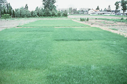
Here is an example from Fowler, Cohen and Parvis (1998). An agriculturalist was interested in the effects of fertilizer load on the yield of grass. Grass seed was sown uniformly over an area and different quantities of commercial fertilizer were applied to each of ten 1 m² randomly located plots. Two months later the grass from each plot was harvested, dried and weighed. The data are in the file fertilizer.csv.

Download Fertilizer data set

Format of fertilizer.csv data files

FERTILIZER	YIELD
25	84
50	80
75	90
100	154
125	148
...	...

FERTILIZER	Mass of fertilizer (g.m^-2) - Predictor variable
YIELD	Yield of grass (g.m^-2) - Response variable

Open

Show code

fert <- read.table('../downloads/data/fertilizer.csv', header=T, sep=',', strip.white=T)
fert

   FERTILIZER YIELD
1          25    84
2          50    80
3          75    90
4         100   154
5         125   148
6         150   169
7         175   206
8         200   244
9         225   212
10        250   248

List the following:
1. The biological hypothesis of interest
2. The biological null hypothesis of interest
3. The statistical null hypothesis of interest
Test the assumptions of simple linear regression using a scatterplot
of YIELD against FERTILIZER. Add boxplots for each variable to the margins and fit a lowess smoother through the data. Is there any evidence of violations of the simple linear regression assumptions? (Y or N)

Show base graphics code
# get the car package library(car) scatterplot(YIELD~FERTILIZER, data=fert)
Show ggplot code
library(tidyverse) ggplot(fert, aes(y=YIELD, x=FERTILIZER)) + geom_point() + geom_smooth()
ggplot(fert, aes(y=YIELD)) + geom_boxplot(aes(x=1))
If there is no evidence that the assumptions of simple linear regression have been violated, fit the linear model
YIELD = intercept + (SLOPE * FERTILIZER). At this stage ignore any output.
Show code
fert.lm<-lm(YIELD~FERTILIZER, data=fert)

Examine the regression diagnostics

(particularly the residual plot

). Does the residual plot indicate any potential problems with the data? (Y or N)

Show base graphics code

# setup a 2x6 plotting device with small margins
par(mfrow = c(2, 3), oma = c(0, 0, 2, 0))
plot(fert.lm,ask=F,which=1:6)

influence.measures(fert.lm)

Influence measures of
 lm(formula = YIELD ~ FERTILIZER, data = fert) :

      dfb.1_ dfb.FERT   dffit cov.r  cook.d   hat inf
1   5.39e-01  -0.4561  0.5411 1.713 0.15503 0.345    
2  -4.15e-01   0.3277 -0.4239 1.497 0.09527 0.248    
3  -6.01e-01   0.4237 -0.6454 0.969 0.18608 0.176    
4   3.80e-01  -0.2145  0.4634 1.022 0.10137 0.127    
5  -5.77e-02   0.0163 -0.0949 1.424 0.00509 0.103    
6  -2.50e-02  -0.0141 -0.0821 1.432 0.00382 0.103    
7   2.09e-17   0.1159  0.2503 1.329 0.03374 0.127    
8  -2.19e-01   0.6184  0.9419 0.623 0.31796 0.176    
9   3.29e-01  -0.6486 -0.8390 1.022 0.30844 0.248    
10  1.51e-01  -0.2559 -0.3035 1.900 0.05137 0.345   *

library(effects)
plot(Effect('FERTILIZER',fert.lm, partial.residuals=TRUE))

Show autoplot code

library(ggfortify)
autoplot(fert.lm, which=1:6)

    influence.measures(fert.lm)

Influence measures of
 lm(formula = YIELD ~ FERTILIZER, data = fert) :

      dfb.1_ dfb.FERT   dffit cov.r  cook.d   hat inf
1   5.39e-01  -0.4561  0.5411 1.713 0.15503 0.345    
2  -4.15e-01   0.3277 -0.4239 1.497 0.09527 0.248    
3  -6.01e-01   0.4237 -0.6454 0.969 0.18608 0.176    
4   3.80e-01  -0.2145  0.4634 1.022 0.10137 0.127    
5  -5.77e-02   0.0163 -0.0949 1.424 0.00509 0.103    
6  -2.50e-02  -0.0141 -0.0821 1.432 0.00382 0.103    
7   2.09e-17   0.1159  0.2503 1.329 0.03374 0.127    
8  -2.19e-01   0.6184  0.9419 0.623 0.31796 0.176    
9   3.29e-01  -0.6486 -0.8390 1.022 0.30844 0.248    
10  1.51e-01  -0.2559 -0.3035 1.900 0.05137 0.345   *

Prior to exploring the model output, it is often a good idea to produce a quick partial plot. This helps appreciate the patterns contained within the fitted model as well as interpreting any estimated parameters/effects.
Show effects code
library(effects) plot(Effect('FERTILIZER',fert.lm, partial.residuals=TRUE))
Show ggpredict code
library(ggeffects) ggpredict(fert.lm, ~FERTILIZER) %>% plot(rawdata=TRUE)
Show ggemmeans code
library(ggeffects) ggemmeans(fert.lm, ~FERTILIZER) %>% plot

If there is no evidence that any of the assumptions have been violated, examine the regression output

. Identify and interpret the following;

Show code

summary(fert.lm)

Call:
lm(formula = YIELD ~ FERTILIZER, data = fert)

Residuals:
   Min     1Q Median     3Q    Max 
-22.79 -11.07  -5.00  12.00  29.79 

Coefficients:
            Estimate Std. Error t value Pr(>|t|)    
(Intercept) 51.93333   12.97904   4.001  0.00394 ** 
FERTILIZER   0.81139    0.08367   9.697 1.07e-05 ***
---
Signif. codes:  0 '***' 0.001 '**' 0.01 '*' 0.05 '.' 0.1 ' ' 1

Residual standard error: 19 on 8 degrees of freedom
Multiple R-squared:  0.9216,	Adjusted R-squared:  0.9118 
F-statistic: 94.04 on 1 and 8 DF,  p-value: 1.067e-05

Show confint code

confint(fert.lm)

                 2.5 %    97.5 %
(Intercept) 22.0036246 81.863042
FERTILIZER   0.6184496  1.004338

Show tidy code

library(broom)
tidy(fert.lm, conf.int=TRUE)

# A tibble: 2 x 7
  term        estimate std.error statistic   p.value conf.low conf.high
  <chr>          <dbl>     <dbl>     <dbl>     <dbl>    <dbl>     <dbl>
1 (Intercept)   51.9     13.0         4.00 0.00394     22.0       81.9 
2 FERTILIZER     0.811    0.0837      9.70 0.0000107    0.618      1.00

sample y-intercept
sample slope
t value for main H₀
R² value

What conclusions (statistical and biological) would you draw from the analysis?

Significant simple linear regression outcomes are usually accompanied by a scatterpoint that summarizes the relationship between the two population. Construct a scatterplot

without marginal boxplots.

Show base graphics code

#setup the graphics device with wider margins
opar <- par(mar=c(5,5,0,0))
#construct the base plot without axes or labels or even points
plot(YIELD~FERTILIZER, data=fert, ann=F, axes=F, type="n")
# put the points on as solid circles (point character 16)
points(YIELD~FERTILIZER, data=fert, pch=16)
# calculate predicted values
xs <- seq(min(fert$FERTILIZER), max(fert$FERTILIZER), l = 1000)
ys <- predict(fert.lm, newdata = data.frame(FERTILIZER = xs), se=T)
lines(xs,ys$fit-ys$se.fit, lty=2)
lines(xs,ys$fit+ys$se.fit, lty=2)
lines(xs, ys$fit)
# draw the x-axis
axis(1)
mtext("Fertilizer concentration",1,line=3)
# draw the y-axis (labels rotated)
axis(2,las=1)
mtext("Grass yield",2,line=3)
#put an 'L'-shaped box around the plot
box(bty="l")

#reset the parameters
par(opar)

Show ggplot code

library(ggplot2)
ggplot(fert, aes(y=YIELD, x=FERTILIZER)) +
  geom_point()+
  geom_smooth(method='lm', fill='blue',alpha=0.2)+
  scale_y_continuous(expression(Grass~yield~(g.m^{-2})))+
  scale_x_continuous(expression(Fertilizer~concentration~(g.m^{-2})))+
  theme_classic()+
  theme(axis.title.y=element_text(vjust=2, size=rel(1.5)),
                axis.title.x=element_text(vjust=-1, size=rel(1.5)))

Show manual code

newdata = with(fert, data.frame(FERTILIZER=seq(min(FERTILIZER), max(FERTILIZER), len=100)))
Xmat = model.matrix(~FERTILIZER, data=newdata)
coefs=coef(fert.lm)
    fit = as.vector(coefs %*% t(Xmat))
SE = sqrt(diag(Xmat %*% vcov(fert.lm) %*% t(Xmat)))
Q = qt(0.975, df=df.residual(fert.lm))
newdata = newdata %>% mutate(lower=fit-Q*SE, upper=fit+Q*SE, fit=fit)

partial.Xmat = model.matrix(~FERTILIZER, data=fert)
partial.resid = fert %>% mutate(Partial=as.vector(coefs %*% t(partial.Xmat)) + resid(fert.lm))
library(ggplot2)
ggplot(newdata, aes(y=fit, x=FERTILIZER)) +
      geom_ribbon(aes(ymin=lower, ymax=upper), fill='blue', color=NA, alpha=0.3) +
      geom_line() +
  geom_point(data=partial.resid, aes(y=Partial))+
  scale_y_continuous(expression(Grass~yield~(g.m^{-2})))+
  scale_x_continuous(expression(Fertilizer~concentration~(g.m^{-2})))+
  theme_classic()+
  theme(axis.title.y=element_text(vjust=2, size=rel(1.5)),
                axis.title.x=element_text(vjust=-1, size=rel(1.5)))

Show emmeans code

fert.grid = with(fert, list(FERTILIZER=seq(min(FERTILIZER), max(FERTILIZER), len=100)))
newdata = ref_grid(fert.lm, ~FERTILIZER, at=fert.grid, cov.reduce=FALSE) %>% confint
partial.resid = ref_grid(fert.lm, ~FERTILIZER, cov.reduce=FALSE) %>% summary %>%
  mutate(Partial=prediction+resid(fert.lm))
library(ggplot2)
ggplot(newdata, aes(y=prediction, x=FERTILIZER)) +
      geom_ribbon(aes(ymin=lower.CL, ymax=upper.CL), fill='blue', color=NA, alpha=0.3) +
      geom_line() +
  geom_point(data=partial.resid, aes(y=Partial))+
  scale_y_continuous(expression(Grass~yield~(g.m^{-2})))+
  scale_x_continuous(expression(Fertilizer~concentration~(g.m^{-2})))+
  theme_classic()+
  theme(axis.title.y=element_text(vjust=2, size=rel(1.5)),
                axis.title.x=element_text(vjust=-1, size=rel(1.5)))

Simple linear regression

Christensen et al. (1996) studied the relationships between coarse woody debris (CWD) and, shoreline vegetation and lake development in a sample of 16 lakes. They defined CWD as debris greater than 5cm in diameter and recorded, for a number of plots on each lake, the basal area (m².km^-1) of CWD in the nearshore water, and the density (no.km^-1) of riparian trees along the shore. The data are in the file christ.csv and the relevant variables are the response variable, CWDBASAL (coarse woody debris basal area, m².km-1), and the predictor variable, RIPDENS (riparian tree density, trees.km^-1).

Download Christensen data set

Format of christ.csv data files

LAKE	RIPDENS	CWDBASAL
Bay	1270	121
Bergner	1210	41
Crampton	1800	183
Long	1875	130
Roach	1300	127
...	...	...

LAKE	Name of the North American freshwater lake from which the observations were collected
RIPDENS	Density of riparian trees (trees.km^-1) Predictor variable
CWDBASAL	Course woody debris basal area (m².km^-1) Response variable

Open the christ data file.

Show code

christ <- read.table('../downloads/data/christ.csv', header=T, sep=',', strip.white=T)
head(christ)

        LAKE RIPDENS CWDBASAL
1        Bay    1270      121
2    Bergner    1210       41
3   Crampton    1800      183
4       Long    1875      130
5      Roach    1300      127
6 Tenderfoot    2150      134

List the following:
1. The biological hypothesis of interest
2. The biological null hypothesis of interest
3. The statistical null hypothesis of interest
In the table below, list the assumptions of simple linear regression along with how violations of each assumption are diagnosed and/or the risks of violations are minimized.

Assumption Diagnostic/Risk Minimization
I.

II.

III.

IV.
Draw a scatterplot
of CWDBASAL against RIPDENS. This should include boxplots for each variable to the margins and a fitted lowess smoother through the data HINT.
Show base graphics code
library(car) scatterplot(CWDBASAL~RIPDENS, data=christ)
Show ggplot code
library(tidyverse) ggplot(christ, aes(y=CWDBASAL, x=RIPDENS)) + geom_point() + geom_smooth()
ggplot(christ, aes(y=CWDBASAL)) + geom_boxplot(aes(x=1))
ggplot(christ, aes(y=RIPDENS)) + geom_boxplot(aes(x=1))
1. Is there any evidence of nonlinearity? (Y or N)
2. Is there any evidence of nonnormality? (Y or N)
3. Is there any evidence of unequal variance? (Y or N)
The main intention of the researchers is to investigate whether there is a linear relationship between the density of riparian vegetation and the size of the logs. They have no of using the model equation for further predictions, not are they particularly interested in the magnitude of the relationship (slope). Is model I or II regression
appropriate in these circumstances?. Explain?

If there is no evidence that the assumptions of simple linear regression have been violated, fit the linear model
CWDBASAL = (SLOPE * RIPDENS) + intercept HINT. At this stage ignore any output.

Show code
christ.lm<-lm(CWDBASAL~RIPDENS, data=christ)

Assumption	Diagnostic/Risk Minimization
I.
II.
III.
IV.

Examine the regression diagnostics

(particularly the residual plot)

HINT. Does the residual plot indicate any potential problems with the data? (Y or N)

Show code

# setup a 2x6 plotting device with small margins
par(mfrow = c(2, 3), oma = c(0, 0, 2, 0))
plot(christ.lm,ask=F,which=1:6)

influence.measures(christ.lm)

Influence measures of
 lm(formula = CWDBASAL ~ RIPDENS, data = christ) :

     dfb.1_ dfb.RIPD  dffit cov.r  cook.d    hat inf
1   0.09523   0.0230  0.396 0.889 0.07148 0.0627    
2  -0.06051   0.0150 -0.156 1.172 0.01280 0.0631    
3  -0.50292   0.6733  0.822 0.958 0.29787 0.1896    
4   0.10209  -0.1323 -0.155 1.480 0.01293 0.2264   *
5   0.06999   0.0568  0.423 0.857 0.08004 0.0637    
6   0.85160  -1.0289 -1.120 1.482 0.59032 0.4016   *
7  -0.00766  -0.0175 -0.084 1.222 0.00377 0.0653    
8   0.13079  -0.0961  0.163 1.235 0.01401 0.0959    
9  -0.16369   0.1207 -0.203 1.211 0.02156 0.0967    
10  0.02294  -0.1138 -0.311 1.042 0.04742 0.0722    
11 -0.02588  -0.0101 -0.120 1.198 0.00763 0.0629    
12  0.49223  -0.3571  0.622 0.769 0.16169 0.0932    
13 -0.12739   0.1065 -0.137 1.355 0.01007 0.1570    
14 -0.15382   0.1248 -0.171 1.301 0.01550 0.1340    
15 -0.21860   0.1721 -0.251 1.224 0.03278 0.1178    
16 -0.22479   0.1666 -0.277 1.156 0.03922 0.0979

library(effects)
plot(Effect('RIPDENS', christ.lm, partial.residuals=TRUE))

Show autoplot code

library(ggfortify)
autoplot(christ.lm, which=1:6)

influence.measures(christ.lm)

Influence measures of
 lm(formula = CWDBASAL ~ RIPDENS, data = christ) :

     dfb.1_ dfb.RIPD  dffit cov.r  cook.d    hat inf
1   0.09523   0.0230  0.396 0.889 0.07148 0.0627    
2  -0.06051   0.0150 -0.156 1.172 0.01280 0.0631    
3  -0.50292   0.6733  0.822 0.958 0.29787 0.1896    
4   0.10209  -0.1323 -0.155 1.480 0.01293 0.2264   *
5   0.06999   0.0568  0.423 0.857 0.08004 0.0637    
6   0.85160  -1.0289 -1.120 1.482 0.59032 0.4016   *
7  -0.00766  -0.0175 -0.084 1.222 0.00377 0.0653    
8   0.13079  -0.0961  0.163 1.235 0.01401 0.0959    
9  -0.16369   0.1207 -0.203 1.211 0.02156 0.0967    
10  0.02294  -0.1138 -0.311 1.042 0.04742 0.0722    
11 -0.02588  -0.0101 -0.120 1.198 0.00763 0.0629    
12  0.49223  -0.3571  0.622 0.769 0.16169 0.0932    
13 -0.12739   0.1065 -0.137 1.355 0.01007 0.1570    
14 -0.15382   0.1248 -0.171 1.301 0.01550 0.1340    
15 -0.21860   0.1721 -0.251 1.224 0.03278 0.1178    
16 -0.22479   0.1666 -0.277 1.156 0.03922 0.0979

Prior to exploring the model output, it is often a good idea to produce a quick partial plot. This helps appreciate the patterns contained within the fitted model as well as interpreting any estimated parameters/effects.
Show base graphics code
library(effects) plot(Effect('RIPDENS',christ.lm, partial.residuals=TRUE))
Show ggpredict code
library(ggeffects) ggpredict(christ.lm, ~RIPDENS) %>% plot(rawdata=TRUE)
Show ggemmeans code
library(ggeffects) ggemmeans(christ.lm, ~RIPDENS) %>% plot

At this point, we have no evidence to suggest that the hypothesis tests will not be reliable. Examine the regression output and identify and interpret the following:

Show code

summary(christ.lm)

Call:
lm(formula = CWDBASAL ~ RIPDENS, data = christ)

Residuals:
   Min     1Q Median     3Q    Max 
-38.62 -22.41 -13.33  26.16  61.35 

Coefficients:
             Estimate Std. Error t value Pr(>|t|)    
(Intercept) -77.09908   30.60801  -2.519 0.024552 *  
RIPDENS       0.11552    0.02343   4.930 0.000222 ***
---
Signif. codes:  0 '***' 0.001 '**' 0.01 '*' 0.05 '.' 0.1 ' ' 1

Residual standard error: 36.32 on 14 degrees of freedom
Multiple R-squared:  0.6345,	Adjusted R-squared:  0.6084 
F-statistic:  24.3 on 1 and 14 DF,  p-value: 0.0002216

Show confint code

confint(christ.lm)

                    2.5 %      97.5 %
(Intercept) -142.74672817 -11.4514274
RIPDENS        0.06525871   0.1657734

Show tidy code

library(broom)
tidy(christ.lm, conf.int=TRUE)

# A tibble: 2 x 7
  term        estimate std.error statistic  p.value  conf.low conf.high
  <chr>          <dbl>     <dbl>     <dbl>    <dbl>     <dbl>     <dbl>
1 (Intercept)  -77.1     30.6        -2.52 0.0246   -143.       -11.5  
2 RIPDENS        0.116    0.0234      4.93 0.000222    0.0653     0.166

sample y-intercept
sample slope
t value for main H₀
P-value for main H₀
R² value

What conclusions (statistical and biological) would you draw from the analysis?

Finally, how about a nice summary figure.

Show base graphics code

#setup the graphics device with wider margins
opar <- par(mar=c(5,5,0,0))
#construct the base plot without axes or labels or even points
plot(CWDBASAL~RIPDENS, data=christ, ann=F, axes=F, type="n")
# put the points on as solid circles (point character 16)
points(CWDBASAL~RIPDENS, data=christ, pch=16)
# calculate predicted values
xs <- seq(min(christ$RIPDENS), max(christ$RIPDENS), l = 1000)
ys <- predict(christ.lm, newdata = data.frame(RIPDENS = xs), se=T)
lines(xs,ys$fit-ys$se.fit, lty=2)
lines(xs,ys$fit+ys$se.fit, lty=2)
lines(xs, ys$fit)
# draw the x-axis
axis(1)
mtext("Density of riparian trees",1,line=3)
# draw the y-axis (labels rotated)
axis(2,las=1)
mtext("Course woody debris basal area",2,line=3)
#put an 'L'-shaped box around the plot
box(bty="l")

#reset the parameters
par(opar)

Show ggplot code

library(ggplot2)
ggplot(christ, aes(y=CWDBASAL, x=RIPDENS)) +
  geom_point()+
  geom_smooth(method='lm', fill='blue',alpha=0.2)+
  scale_y_continuous(expression(Density~of~riparian~trees~(trees.km^{-1})))+
  scale_x_continuous(expression(Course~woody~debris~basal~area~(m^2~km^{-1})))+
  theme_classic()+
  theme(axis.title.y=element_text(vjust=2, size=rel(1.5)),
        axis.title.x=element_text(vjust=-1, size=rel(1.5)))

Show manual code

newdata = with(christ, data.frame(RIPDENS=seq(min(RIPDENS), max(RIPDENS), len=100)))
Xmat = model.matrix(~RIPDENS, data=newdata)
coefs=coef(christ.lm)
    fit = as.vector(coefs %*% t(Xmat))
SE = sqrt(diag(Xmat %*% vcov(christ.lm) %*% t(Xmat)))
Q = qt(0.975, df=df.residual(christ.lm))
newdata = newdata %>% mutate(lower=fit-Q*SE, upper=fit+Q*SE, fit=fit)

partial.Xmat = model.matrix(~RIPDENS, data=christ)
partial.resid = christ %>% mutate(Partial=as.vector(coefs %*% t(partial.Xmat)) + resid(christ.lm))
library(ggplot2)
ggplot(newdata, aes(y=fit, x=RIPDENS)) +
      geom_ribbon(aes(ymin=lower, ymax=upper), fill='blue', color=NA, alpha=0.3) +
      geom_line() +
  geom_point(data=partial.resid, aes(y=Partial))+
  scale_y_continuous(expression(Density~of~riparian~trees~(trees.km^{-1})))+
  scale_x_continuous(expression(Course~woody~debris~basal~area~(m^2~km^{-1})))+
  theme_classic()+
  theme(axis.title.y=element_text(vjust=2, size=rel(1.5)),
                axis.title.x=element_text(vjust=-1, size=rel(1.5)))

Simple linear regression

Here is a modified example from Quinn and Keough (2002). Peake & Quinn (1993) investigated the relationship between the number of individuals of invertebrates living in amongst clumps of mussels on a rocky intertidal shore and the area of those mussel clumps.

Download PeakeQuinn data set

Format of peakquinn.csv data files

AREA	INDIV
516.00	18
469.06	60
462.25	57
938.60	100
1357.15	48
...	...

AREA	Area of mussel clump mm² - Predictor variable
INDIV	Number of individuals found within clump - Response variable

Open the peakquinn data file.

Show code

peakquinn <- read.table('../downloads/data/peakquinn.csv', header=T, sep=',', strip.white=T)
peakquinn

       AREA INDIV
1    516.00    18
2    469.06    60
3    462.25    57
4    938.60   100
5   1357.15    48
6   1773.66   118
7   1686.01   148
8   1786.29   214
9   3090.07   225
10  3980.12   283
11  4424.84   380
12  4451.68   278
13  4982.89   338
14  4450.86   274
15  5490.74   569
16  7476.21   509
17  7138.82   682
18  9149.94   600
19 10133.07   978
20  9287.69   363
21 13729.13  1402
22 20300.77   675
23 24712.72  1159
24 27144.03  1062
25 26117.81   632

The relationship between two continuous variables can be analyzed by simple linear regression. As with question 2, note that the levels of the predictor variable were measured, not fixed, and thus parameter estimates should be based on model II RMA regression. Note however, that the hypothesis test for slope is uneffected by whether the predictor variable is fixed or measured.

Before performing the analysis we need to check the assumptions. To evaluate the assumptions of linearity, normality and homogeneity of variance, construct a scatterplot

of INDIV against AREA (INDIV on y-axis, AREA on x-axis) including a lowess smoother and boxplots on the axes.

Show base graphics code

library(car)
scatterplot(INDIV~AREA,data=peakquinn)

Show ggplot code

    library(tidyverse)
ggplot(peakquinn, aes(y=INDIV, x=AREA)) + geom_point() + geom_smooth()

ggplot(peakquinn, aes(y=INDIV)) + geom_boxplot(aes(x=1))

ggplot(peakquinn, aes(y=INDIV, x=AREA)) + geom_point() + geom_smooth() + scale_x_log10() + scale_y_log10()

ggplot(peakquinn, aes(y=INDIV)) + geom_boxplot(aes(x=1)) + scale_y_log10()

ggplot(peakquinn, aes(y=AREA)) + geom_boxplot(aes(x=1)) + scale_y_log10()

Consider the assumptions and suitability of the data for simple linear regression:
1. In this case, the researchers are interested in investigating whether there is a relationship between the number of invertebrate individuals and mussel clump area as well as generating a predictive model. However, they are not interested in the specific magnitude of the relationship (slope) and have no intension of comparing their slope to any other non-zero values. Is model I or II regression
  appropriate in these circumstances?. Explain?
2. Is there any evidence that the other assumptions are likely to be violated?
To get an appreciation of what a residual plot would look like when there is some evidence that the assumption of homogeneity of variance assumption has been violated, perform the simple linear regression (by fitting a linear model)

Show code
peakquinn.lm<-lm(INDIV~AREA, data=peakquinn)

examining the regression diagnostics

residual plot

Show code

# setup a 2x6 plotting device with small margins
par(mfrow = c(2, 3), oma = c(0, 0, 2, 0))
plot(peakquinn.lm,ask=F,which=1:6)

influence.measures(peakquinn.lm)

Influence measures of
 lm(formula = INDIV ~ AREA, data = peakquinn) :

    dfb.1_ dfb.AREA    dffit cov.r   cook.d    hat inf
1  -0.1999  0.13380 -0.20006 1.125 2.04e-02 0.0724    
2  -0.1472  0.09887 -0.14731 1.150 1.12e-02 0.0728    
3  -0.1507  0.10121 -0.15073 1.148 1.17e-02 0.0728    
4  -0.1153  0.07466 -0.11549 1.155 6.92e-03 0.0687    
5  -0.1881  0.11765 -0.18896 1.117 1.82e-02 0.0653    
6  -0.1214  0.07306 -0.12237 1.142 7.75e-03 0.0622    
7  -0.0858  0.05206 -0.08639 1.155 3.88e-03 0.0628    
8  -0.0176  0.01059 -0.01776 1.165 1.65e-04 0.0621    
9  -0.0509  0.02633 -0.05236 1.150 1.43e-03 0.0535    
10 -0.0237  0.01069 -0.02504 1.148 3.28e-04 0.0489    
11  0.0475 -0.01961  0.05096 1.141 1.35e-03 0.0470    
12 -0.0418  0.01717 -0.04492 1.142 1.05e-03 0.0468    
13 -0.0061  0.00221 -0.00672 1.144 2.36e-05 0.0448    
14 -0.0453  0.01859 -0.04862 1.142 1.23e-03 0.0468    
15  0.1641 -0.05100  0.18584 1.067 1.74e-02 0.0433    
16  0.0472 -0.00254  0.06317 1.129 2.08e-03 0.0401    
17  0.1764 -0.01859  0.22781 1.021 2.57e-02 0.0403    
18  0.0542  0.01493  0.09093 1.120 4.28e-03 0.0411    
19  0.2173  0.12011  0.43430 0.808 8.29e-02 0.0433    
20 -0.0701 -0.02168 -0.12016 1.106 7.43e-03 0.0413    
21  0.1849  0.63635  1.07759 0.357 3.36e-01 0.0614   *
22  0.0752 -0.33126 -0.39474 1.157 7.79e-02 0.1352    
23 -0.0789  0.22611  0.25071 1.362 3.25e-02 0.2144   *
24  0.0853 -0.21744 -0.23573 1.473 2.88e-02 0.2681   *
25  0.4958 -1.32133 -1.44477 0.865 8.44e-01 0.2445   *

library(effects)
plot(Effect('AREA', peakquinn.lm, partial.residuals=TRUE))

Show autoplot code

library(ggfortify)
autoplot(peakquinn.lm, which=1:6)

influence.measures(peakquinn.lm)

Influence measures of
 lm(formula = INDIV ~ AREA, data = peakquinn) :

    dfb.1_ dfb.AREA    dffit cov.r   cook.d    hat inf
1  -0.1999  0.13380 -0.20006 1.125 2.04e-02 0.0724    
2  -0.1472  0.09887 -0.14731 1.150 1.12e-02 0.0728    
3  -0.1507  0.10121 -0.15073 1.148 1.17e-02 0.0728    
4  -0.1153  0.07466 -0.11549 1.155 6.92e-03 0.0687    
5  -0.1881  0.11765 -0.18896 1.117 1.82e-02 0.0653    
6  -0.1214  0.07306 -0.12237 1.142 7.75e-03 0.0622    
7  -0.0858  0.05206 -0.08639 1.155 3.88e-03 0.0628    
8  -0.0176  0.01059 -0.01776 1.165 1.65e-04 0.0621    
9  -0.0509  0.02633 -0.05236 1.150 1.43e-03 0.0535    
10 -0.0237  0.01069 -0.02504 1.148 3.28e-04 0.0489    
11  0.0475 -0.01961  0.05096 1.141 1.35e-03 0.0470    
12 -0.0418  0.01717 -0.04492 1.142 1.05e-03 0.0468    
13 -0.0061  0.00221 -0.00672 1.144 2.36e-05 0.0448    
14 -0.0453  0.01859 -0.04862 1.142 1.23e-03 0.0468    
15  0.1641 -0.05100  0.18584 1.067 1.74e-02 0.0433    
16  0.0472 -0.00254  0.06317 1.129 2.08e-03 0.0401    
17  0.1764 -0.01859  0.22781 1.021 2.57e-02 0.0403    
18  0.0542  0.01493  0.09093 1.120 4.28e-03 0.0411    
19  0.2173  0.12011  0.43430 0.808 8.29e-02 0.0433    
20 -0.0701 -0.02168 -0.12016 1.106 7.43e-03 0.0413    
21  0.1849  0.63635  1.07759 0.357 3.36e-01 0.0614   *
22  0.0752 -0.33126 -0.39474 1.157 7.79e-02 0.1352    
23 -0.0789  0.22611  0.25071 1.362 3.25e-02 0.2144   *
24  0.0853 -0.21744 -0.23573 1.473 2.88e-02 0.2681   *
25  0.4958 -1.32133 -1.44477 0.865 8.44e-01 0.2445   *

How would you describe the residual plot?
What could be done to the data to address the problems highlighted by the scatterplot, boxplots and residuals?
Describe how the scatterplot, axial boxplots and residual plot might appear following successful data transformation.

Transform

HINT

Show code

library(car)
scatterplot(log10(INDIV)~log10(AREA), data=peakquinn)

Show ggplot code

    library(tidyverse)
ggplot(peakquinn, aes(y=INDIV, x=AREA)) + geom_point() + geom_smooth() + scale_x_log10() + scale_y_log10()

ggplot(peakquinn, aes(y=INDIV)) + geom_boxplot(aes(x=1)) + scale_y_log10()

ggplot(peakquinn, aes(y=AREA)) + geom_boxplot(aes(x=1)) + scale_y_log10()

Would you consider the transformation as successful? (Y or N)

Note, rather than transform the response so that it conforms to the assumptions of normality, arguably, it would be more appropriate to model these data against a more suitable distribution. In this case, since the response represents count data, a Poisson distribution would be more appropriate than a Gaussian (normal) distribution. Indeed this is the approach that we will take in Tutorial 9.4a. However, for this tutorial, we will fit the normalized data against a normal distribution.

If you are satisfied that the assumptions of the analysis are likely to have been met, perform the linear regression analysis (refit the linear model) HINT, examine the output.

Show model fitting code

peakquinn.lm<-lm(log(INDIV)~log(AREA), data=peakquinn)

Show base graphics diagnostics code

par(mfrow = c(2, 3), oma = c(0, 0, 2, 0))
plot(christ.lm,ask=F,which=1:6)

Show autoplot code

autoplot(peakquinn.lm, which=1:6)

Show effects code

library(effects)
plot(Effect('AREA', peakquinn.lm, partial.residuals=TRUE))

plot(allEffects(peakquinn.lm), partial.residuals=TRUE,
 axes=list(x=list(AREA=list(transform=list(trans=log, inverse=exp),
                            ticks=list(at=c(500,1000,2000,5000,10000, 20000)))),
           y=list(transform=list(transform=exp))))

Error in get(as.character(FUN), mode = "function", envir = envir): object 'inverse' of mode 'function' was not found

Show ggpredict code

library(ggeffects)
ggpredict(peakquinn.lm, term='AREA [exp]') %>% plot() + scale_y_log10() + scale_x_log10()

## The following should work, but there is a bug
ggpredict(peakquinn.lm, term='AREA',full.data=TRUE) %>% plot(rawdata=TRUE)

Show ggemmeans code

library(ggeffects)
ggemmeans(peakquinn.lm, 'AREA [exp]') %>% plot()

ggemmeans(peakquinn.lm, 'AREA [exp]') %>% plot() + scale_x_log10() + scale_y_log10()

Show summary code

summary(peakquinn.lm)

Call:
lm(formula = log(INDIV) ~ log(AREA), data = peakquinn)

Residuals:
    Min      1Q  Median      3Q     Max 
-0.9983 -0.1488  0.0511  0.2574  0.6175 

Coefficients:
            Estimate Std. Error t value Pr(>|t|)    
(Intercept) -1.32632    0.59645  -2.224   0.0363 *  
log(AREA)    0.83492    0.07066  11.816 3.01e-11 ***
---
Signif. codes:  0 '***' 0.001 '**' 0.01 '*' 0.05 '.' 0.1 ' ' 1

Residual standard error: 0.4274 on 23 degrees of freedom
Multiple R-squared:  0.8586,	Adjusted R-squared:  0.8524 
F-statistic: 139.6 on 1 and 23 DF,  p-value: 3.007e-11

Show confint code

confint(peakquinn.lm)

                 2.5 %      97.5 %
(Intercept) -2.5601791 -0.09246238
log(AREA)    0.6887433  0.98108798

Show tidy code

tidy(peakquinn.lm,confint=TRUE)

# A tibble: 2 x 5
  term        estimate std.error statistic  p.value
  <chr>          <dbl>     <dbl>     <dbl>    <dbl>
1 (Intercept)   -1.33     0.596      -2.22 3.63e- 2
2 log(AREA)      0.835    0.0707     11.8  3.01e-11

Test the null hypothesis that the population slope of the regression line between log number of individuals and log clump area is zero - use either the t-test or ANOVA F-test regression output. What are your conclusions (statistical and biological)? HINT
If the relationship is significant construct the regression equation relating the number of individuals in the a clump to the clump size. Remember that parameter estimates should be based on RMA regression not OLS!

DV = intercept + slope x IV

Log_eIndividuals Log_eArea

Write the results out as though you were writing a research paper/thesis. For example (select the phrase that applies and fill in gaps with your results):
A linear regression of log number of individuals against log clump area showed (choose correct option)
(b = , t = , df = , P = )
How much of the variation in log individual number is explained by the linear relationship with log clump area? That is , what is the R² value?

What number of individuals would you predict

for a new clump with an area of 8000 mm²? HINT

Show predict code

#include prediction intervals
exp(predict(peakquinn.lm, newdata=data.frame(AREA=8000), interval="predict"))

       fit      lwr      upr
1 481.6561 194.5975 1192.167

#include 95% confidence intervals
exp(predict(peakquinn.lm, newdata=data.frame(AREA=8000), interval="confidence"))

       fit      lwr      upr
1 481.6561 394.5162 588.0434

Show emmeans code

peakquinn.grid = ref_grid(peakquinn.lm, at=list(AREA=8000))
confint(peakquinn.grid, type='response') %>% as.data.frame

  AREA response       SE df lower.CL upper.CL
1 8000 481.6561 46.46698 23 394.5162 588.0434

Given that in this case both response and predictor variables were measured (the levels of the predictor variable were not specifically set by the researchers), it might be worth presenting the less biased model parameters (y-intercept and slope) from RMA model II regression. Perform the RMA model II regression
and examine the slope and intercept
1. b (slope):
2. c (y-intercept):
Show code
library(lmodel2)
Error in library(lmodel2): there is no package called 'lmodel2'
peakquinn.lm2 <- lmodel2(log10(INDIV)~log10(AREA), data=peakquinn)
Error in lmodel2(log10(INDIV) ~ log10(AREA), data = peakquinn): could not find function "lmodel2"
peakquinn.lm2
Error in eval(expr, envir, enclos): object 'peakquinn.lm2' not found

Significant simple linear regression outcomes are usually accompanied by a scatterplot that summarizes the relationship between the two population. Construct a scatterplot

without a smoother or marginal boxplots. Consider whether or not transformed or untransformed data should be used in this graph.

Show base graphics code

#setup the graphics device with wider margins
opar <- par(mar=c(6,6,0,0))
#construct the base plot with log scale axes 
plot(INDIV~AREA, data=peakquinn, log='xy', ann=F, axes=F, type="n")
# put the points on as solid circles (point character 16)
points(INDIV~AREA, data=peakquinn, pch=16)
# draw the x-axis
axis(1)
mtext(expression(paste("Mussel clump area ",(mm^2))),1,line=4,cex=2)
# draw the y-axis (labels rotated)
axis(2,las=1)
mtext("Number of individuals per clump",2,line=4,cex=2)
#put in the fitted regression trendline
xs <- seq(min(peakquinn$AREA), max(peakquinn$AREA), l = 1000)
ys <- 10^predict(peakquinn.lm, newdata=data.frame(AREA=xs), interval='c')
lines(ys[,'fit']~xs)
matlines(xs,ys, lty=2,col=1)
# include the equation
text(max(peakquinn$AREA), 20, expression(paste(log[10], "INDIV = 0.835.",log[10], "AREA - 0.576")),
  pos = 2)
text(max(peakquinn$AREA), 17, expression(paste(R^2 == 0.857)), pos = 2)
#put an 'L'-shaped box around the plot
box(bty="l")

#reset the parameters
par(opar)

Show ggplot code

library(ggplot2)
library(scales)
ggplot(peakquinn, aes(y=INDIV, x=AREA)) +
  geom_point()+
  geom_smooth(method='lm', fill='blue',alpha=0.2)+
  scale_y_log10(expression(Number~of~individuals), breaks=as.vector(c(1,2,5,10) %o% 10^(-1:2)))+
  scale_x_log10(expression(Mussel~clump~area~(mm^2)), breaks=as.vector(c(1,2,5,10) %o% 10^(-1:5)))+
  theme_classic()+
  theme(axis.title.y=element_text(vjust=2, size=rel(1.5)),
        axis.title.x=element_text(vjust=-1, size=rel(1.5)))

Show manual code

newdata = with(peakquinn, data.frame(AREA=seq(min(AREA), max(AREA), len=100)))
Xmat = model.matrix(~log(AREA), data=newdata)
coefs=coef(peakquinn.lm)
   fit = as.vector(coefs %*% t(Xmat))
SE = sqrt(diag(Xmat %*% vcov(peakquinn.lm) %*% t(Xmat)))
Q = qt(0.975, df=df.residual(peakquinn.lm))
newdata = newdata %>% mutate(lower=exp(fit-Q*SE), upper=exp(fit+Q*SE), fit=exp(fit))

partial.Xmat = model.matrix(~log(AREA), data=peakquinn)
partial.resid = peakquinn %>% mutate(Partial=exp(as.vector(coefs %*% t(partial.Xmat)) + resid(peakquinn.lm)))
library(ggplot2)
ggplot(newdata, aes(y=fit, x=AREA)) +
  geom_ribbon(aes(ymin=lower, ymax=upper), fill='blue', color=NA, alpha=0.3) +
  geom_line() +
  geom_point(data=partial.resid, aes(y=Partial))+
  scale_y_log10(expression(Grass~yield~(g.m^{-2})))+
  scale_x_log10(expression(Fertilizer~concentration~(g.m^{-2})))+
  theme_classic()+
  theme(axis.title.y=element_text(vjust=2, size=rel(1.5)),
                axis.title.x=element_text(vjust=-1, size=rel(1.5)))

Show emmeans code

peakquinn.grid = with(peakquinn, list(AREA=seq(min(AREA), max(AREA), len=100)))
newdata = ref_grid(peakquinn.lm, ~AREA, at=peakquinn.grid, cov.reduce=FALSE) %>% confint(type='response')
partial.resid = ref_grid(peakquinn.lm, ~AREA, cov.reduce=FALSE) %>% summary %>%
  mutate(Partial=exp(prediction+resid(peakquinn.lm)))
library(ggplot2)
ggplot(newdata, aes(y=response, x=AREA)) +
  geom_ribbon(aes(ymin=lower.CL, ymax=upper.CL), fill='blue', color=NA, alpha=0.3) +
  geom_line() +
  geom_point(data=partial.resid, aes(y=Partial))+
  scale_y_log10(expression(Grass~yield~(g.m^{-2})))+
  scale_x_log10(expression(Fertilizer~concentration~(g.m^{-2})))+
  theme_classic()+
  theme(axis.title.y=element_text(vjust=2, size=rel(1.5)),
                axis.title.x=element_text(vjust=-1, size=rel(1.5)))

Model II RMA regression

Nagy, Girard & Brown (1999) investigated the allometric scaling relationships for mammals (79 species), reptiles (55 species) and birds (95 species). The observed relationships between body size and metabolic rates of organisms have attracted a great deal of discussion amongst scientists from a wide range of disciplines recently. Whilst some have sort to explore explanations for the apparently 'universal' patterns, Nagy et al. (1999) were interested in determining whether scaling relationships differed between taxonomic, dietary and habitat groupings.

Download Nagy data set

Format of nagy.csv data file

Species	Common	Mass	FMR	Taxon	Habitat	Diet	Class
Pipistrellus pipistrellus	Pipistrelle	7.3	29.3	Ch	ND	I	Mammal
Plecotus auritus	Brown long-eared bat	8.5	27.6	Ch	ND	I	Mammal
Myotis lucifugus	Little brown bat	9.0	29.9	Ch	ND	I	Mammal
Gerbillus henleyi	Northern pygmy gerbil	9.3	26.5	Ro	D	G	Mammal
Tarsipes rostratus	Honey possum	9.9	34.4	Tr	ND	N	Mammal
..	..	..	..	..	..	..	..

Open the nagy data file.

Show code

nagy <- read.table('../downloads/data/nagy.csv', header=T, sep=',', strip.white=T)
head(nagy)

                    Species                Common Mass  FMR Taxon Habitat Diet  Class   MASS
1 Pipistrellus pipistrellus           Pipistrelle  7.3 29.3    Ch      ND    I Mammal 0.0073
2          Plecotus auritus  Brown long-eared bat  8.5 27.6    Ch      ND    I Mammal 0.0085
3          Myotis lucifugus      Little brown bat  9.0 29.9    Ch      ND    I Mammal 0.0090
4         Gerbillus henleyi Northern pygmy gerbil  9.3 26.5    Ro       D    G Mammal 0.0093
5        Tarsipes rostratus          Honey possum  9.9 34.4    Tr      ND    N Mammal 0.0099
6           Anoura caudifer   Flower-visiting bat 11.5 51.9    Ch      ND    N Mammal 0.0115

For this example, we will explore the relationships between field metabolic rate (FMR) and body mass (Mass) in grams for the entire data set and then separately for each of the three classes (mammals, reptiles and aves).

Unlike the previous examples in which both predictor and response variables could be considered 'random' (measured not set), parameter estimates should be based on model II RMA regression. However, unlike previous examples, in this example, the primary focus is not hypothesis testing about whether there is a relationship or not. Nor is prediction a consideration. Instead, the researchers are interested in establishing (and comparing) the allometric scaling factors (slopes) of the metabolic rate - body mass relationships. Hence in this case, model II regression is indeed appropriate.

Before performing the analysis we need to check the assumptions. To evaluate the assumptions of linearity, normality and homogeneity of variance, construct a scatterplot
of FMR against Mass including a lowess smoother and boxplots on the axes.
Show code
library(car) scatterplot(FMR~Mass,data=nagy)
1. Is there any evidence of non-normality?
2. Is there any evidence of non-linearity?
Typically, allometric scaling data are treated by a log-log transformation. That is, both predictor and response variables are log₁₀ transformed. This is achieved graphically on a scatterplot by plotting the data on log transformed axes. Produce such a scatterplot (HINT). Does this improve linearity?
Show code
library(car) scatterplot(FMR~Mass,data=nagy,log='xy')

Fit the linear models relating log-log transformed FMR and Mass using both the Ordinary Least Squares and Reduced Major Axis methods separately for each of the classes (mammals, reptiles and aves).

Show code

nagy.olsM <- lm(log10(FMR)~log10(Mass),data=subset(nagy,nagy$Class=="Mammal"))
summary(nagy.olsM)

Call:
lm(formula = log10(FMR) ~ log10(Mass), data = subset(nagy, nagy$Class == 
    "Mammal"))

Residuals:
     Min       1Q   Median       3Q      Max 
-0.60271 -0.13172 -0.00811  0.14440  0.41794 

Coefficients:
            Estimate Std. Error t value Pr(>|t|)    
(Intercept)  0.68301    0.05336   12.80   <2e-16 ***
log10(Mass)  0.73412    0.01924   38.15   <2e-16 ***
---
Signif. codes:  0 '***' 0.001 '**' 0.01 '*' 0.05 '.' 0.1 ' ' 1

Residual standard error: 0.2119 on 77 degrees of freedom
Multiple R-squared:  0.9498,	Adjusted R-squared:  0.9491 
F-statistic:  1456 on 1 and 77 DF,  p-value: < 2.2e-16

nagy.olsR <- lm(log10(FMR)~log10(Mass),data=subset(nagy,nagy$Class=="Reptiles"))
summary(nagy.olsR)

Call:
lm(formula = log10(FMR) ~ log10(Mass), data = subset(nagy, nagy$Class == 
    "Reptiles"))

Residuals:
     Min       1Q   Median       3Q      Max 
-0.61438 -0.07813 -0.00782  0.17257  0.39794 

Coefficients:
            Estimate Std. Error t value Pr(>|t|)    
(Intercept) -0.70658    0.05941  -11.89   <2e-16 ***
log10(Mass)  0.88789    0.02941   30.19   <2e-16 ***
---
Signif. codes:  0 '***' 0.001 '**' 0.01 '*' 0.05 '.' 0.1 ' ' 1

Residual standard error: 0.2289 on 53 degrees of freedom
Multiple R-squared:  0.945,	Adjusted R-squared:  0.944 
F-statistic: 911.5 on 1 and 53 DF,  p-value: < 2.2e-16

nagy.olsA <- lm(log10(FMR)~log10(Mass),data=subset(nagy,nagy$Class=="Aves"))
summary(nagy.olsA)

Call:
lm(formula = log10(FMR) ~ log10(Mass), data = subset(nagy, nagy$Class == 
    "Aves"))

Residuals:
     Min       1Q   Median       3Q      Max 
-0.53281 -0.07884  0.00453  0.09973  0.41202 

Coefficients:
            Estimate Std. Error t value Pr(>|t|)    
(Intercept)  1.01945    0.03929   25.95   <2e-16 ***
log10(Mass)  0.68079    0.01817   37.46   <2e-16 ***
---
Signif. codes:  0 '***' 0.001 '**' 0.01 '*' 0.05 '.' 0.1 ' ' 1

Residual standard error: 0.1653 on 93 degrees of freedom
Multiple R-squared:  0.9378,	Adjusted R-squared:  0.9372 
F-statistic:  1403 on 1 and 93 DF,  p-value: < 2.2e-16

library(lmodel2)

Error in library(lmodel2): there is no package called 'lmodel2'

nagy.rmaM <- lmodel2(log10(FMR)~log10(Mass),data=subset(nagy,nagy$Class=="Mammal"), nperm=99, range.y='interval', range.x='interval')

Error in lmodel2(log10(FMR) ~ log10(Mass), data = subset(nagy, nagy$Class == : could not find function "lmodel2"

nagy.rmaM

Error in eval(expr, envir, enclos): object 'nagy.rmaM' not found

nagy.rmaR <- lmodel2(log10(FMR)~log10(Mass),data=subset(nagy,nagy$Class=="Reptiles"), nperm=99, range.y='interval', range.x='interval')

Error in lmodel2(log10(FMR) ~ log10(Mass), data = subset(nagy, nagy$Class == : could not find function "lmodel2"

nagy.rmaR

Error in eval(expr, envir, enclos): object 'nagy.rmaR' not found

nagy.rmaA <- lmodel2(log10(FMR)~log10(Mass),data=subset(nagy,nagy$Class=="Aves"), nperm=99, range.y='interval', range.x='interval')

Error in lmodel2(log10(FMR) ~ log10(Mass), data = subset(nagy, nagy$Class == : could not find function "lmodel2"

nagy.rmaA

Error in eval(expr, envir, enclos): object 'nagy.rmaA' not found

Indicate the following;

	OLS		RMA
Class	Slope	Intercept	Slope	Intercept	R²
Mammals (HINT and HINT)
Reptiles ( HINT and HINT)
Aves (HINT and HINT)

Produce a scatterplot that depicts the relationship between FMR and Mass just for the mammals (HINT)

Fit the OLS regression line to this plot (HINT)
Fit the RMA regression line (in red) to this plot (HINT)

Show code

#setup the graphics device with wider margins
opar <- par(mar=c(6,6,0,0))
#construct the base plot with log scale axes
plot(FMR~Mass,data=subset(nagy,nagy$Class=="Mammal"), log='xy', ann=F, axes=F, type="n")
# put the points on as solid circles (point character 16)
points(FMR~Mass,data=subset(nagy,nagy$Class=="Mammal"), pch=16)
# draw the x-axis
axis(1)
mtext(expression(paste("Mass ",(g))),1,line=4,cex=2)
# draw the y-axis (labels rotated)
axis(2,las=1)
mtext("Field metabolic rate",2,line=4,cex=2)
#put in the fitted regression trendline
xs <- with(subset(nagy,nagy$Class=="Mammal"),seq(min(Mass), max(Mass), l = 1000))
ys <- 10^predict(nagy.olsM, newdata=data.frame(Mass=xs), interval='c')
lines(ys[,'fit']~xs)
matlines(xs,ys, lty=2,col=1)
#now include the RMA trendline
centr.y <- mean(nagy.rmaM$y)

Error in mean(nagy.rmaM$y): object 'nagy.rmaM' not found

centr.x <- mean(nagy.rmaM$x)

Error in mean(nagy.rmaM$x): object 'nagy.rmaM' not found

A <- nagy.rmaM$regression.results[4,2]

Error in eval(expr, envir, enclos): object 'nagy.rmaM' not found

B <- nagy.rmaM$regression.results[4,3]

Error in eval(expr, envir, enclos): object 'nagy.rmaM' not found

B1 <- nagy.rmaM$confidence.intervals[4, 4]

Error in eval(expr, envir, enclos): object 'nagy.rmaM' not found

A1 <- centr.y - B1 * centr.x

Error in eval(expr, envir, enclos): object 'centr.y' not found

B2 <- nagy.rmaM$confidence.intervals[4, 5]

Error in eval(expr, envir, enclos): object 'nagy.rmaM' not found

A2 <- centr.y - B2 * centr.x

Error in eval(expr, envir, enclos): object 'centr.y' not found

lines(10^(A+(log10(xs)*B))~xs, col="red")

Error in eval(predvars, data, env): object 'A' not found

lines(10^(A1+(log10(xs)*B1))~xs, col="red",lty=2)

Error in eval(predvars, data, env): object 'A1' not found

lines(10^(A2+(log10(xs)*B2))~xs, col="red",lty=2)

Error in eval(predvars, data, env): object 'A2' not found

# include the equation
#text(max(peakquinn$AREA), 20, expression(paste(log[10], "INDIV = 0.835.",log[10], "AREA - 0.576")), pos = 2)
#text(max(peakquinn$AREA), 17, expression(paste(R^2 == 0.857)), pos = 2)
##put an 'L'-shaped box around the plot
box(bty="l")

#reset the parameters
par(opar)

Compare and contrast the OLS and RMA parameter estimates. Explain which estimates are most appropriate and why the in this case the two methods produce very similar estimates.

To see how the degree of correlation can impact on the difference between OLS and RMA estimates, fit the relationship between FMR and Mass for the entire data set.

Show code

library(lmodel2)

Error in library(lmodel2): there is no package called 'lmodel2'

nagy.rma <- lmodel2(log10(FMR)~log10(Mass),data=nagy, nperm=99, range.y='interval', range.x='interval')

Error in lmodel2(log10(FMR) ~ log10(Mass), data = nagy, nperm = 99, range.y = "interval", : could not find function "lmodel2"

nagy.rma

Error in eval(expr, envir, enclos): object 'nagy.rma' not found

Complete the following table

OLS RMA

Class Slope Intercept Slope Intercept R²
Entire data set (HINT and HINT)
Produce a scatterplot that depicts the relationship between FMR and Mass for the entire data set (HINT)
Fit the OLS regression line to this plot (HINT)
Fit the RMA regression line (in red) to this plot (HINT)
Compare and contrast the OLS and RMA parameter estimates. Explain which estimates are most appropriate and why the in this case the two methods produce not so similar estimates.

Show code

#setup the graphics device with wider margins
opar <- par(mar=c(6,6,0,0))
#construct the base plot with log scale axes
plot(FMR~Mass,data=nagy, log='xy', ann=F, axes=F, type="n")
# put the points on as solid circles (point character 16)
points(FMR~Mass,data=nagy, pch=16)
# draw the x-axis
axis(1)
mtext(expression(paste("Mass ",(g))),1,line=4,cex=2)
# draw the y-axis (labels rotated)
axis(2,las=1)
mtext("Field metabolic rate",2,line=4,cex=2)
#put in the fitted regression trendline
xs <- with(nagy,seq(min(Mass), max(Mass), l = 1000))
nagy.lm<-lm(log10(FMR)~log10(Mass), data=nagy)
ys <- 10^predict(nagy.lm, newdata=data.frame(Mass=xs), interval='c')
lines(ys[,'fit']~xs)
matlines(xs,ys, lty=2,col=1)
#now include the RMA trendline
centr.y <- mean(nagy.rma$y)

Error in mean(nagy.rma$y): object 'nagy.rma' not found

centr.x <- mean(nagy.rma$x)

Error in mean(nagy.rma$x): object 'nagy.rma' not found

A <- nagy.rma$regression.results[4,2]

Error in eval(expr, envir, enclos): object 'nagy.rma' not found

B <- nagy.rma$regression.results[4,3]

Error in eval(expr, envir, enclos): object 'nagy.rma' not found

B1 <- nagy.rma$confidence.intervals[4, 4]

Error in eval(expr, envir, enclos): object 'nagy.rma' not found

A1 <- centr.y - B1 * centr.x

Error in eval(expr, envir, enclos): object 'centr.y' not found

B2 <- nagy.rma$confidence.intervals[4, 5]

Error in eval(expr, envir, enclos): object 'nagy.rma' not found

A2 <- centr.y - B2 * centr.x

Error in eval(expr, envir, enclos): object 'centr.y' not found

lines(10^(A+(log10(xs)*B))~xs, col="red")

Error in eval(predvars, data, env): object 'A' not found

lines(10^(A1+(log10(xs)*B1))~xs, col="red",lty=2)

Error in eval(predvars, data, env): object 'A1' not found

lines(10^(A2+(log10(xs)*B2))~xs, col="red",lty=2)

Error in eval(predvars, data, env): object 'A2' not found

#put an 'L'-shaped box around the plot
box(bty="l")

#reset the parameters
par(opar)

Show code

library(ggplot2)
library(lmodel2)

Error in library(lmodel2): there is no package called 'lmodel2'

dat <- nagy
dat$FMR <- log10(dat$FMR)
dat$Mass <- log10(dat$MASS)
mod.mam <- lmodel2(FMR ~ Mass, data=subset(dat, Class=="Mammal"),"interval", "interval", 99)

Error in lmodel2(FMR ~ Mass, data = subset(dat, Class == "Mammal"), "interval", : could not find function "lmodel2"

mod.rep <- lmodel2(FMR ~ Mass, data=subset(dat, Class=="Reptiles"),"interval", "interval", 99)

Error in lmodel2(FMR ~ Mass, data = subset(dat, Class == "Reptiles"), : could not find function "lmodel2"

mod.ave <- lmodel2(FMR ~ Mass, data=subset(dat, Class=="Aves"),"interval", "interval", 99)

Error in lmodel2(FMR ~ Mass, data = subset(dat, Class == "Aves"), "interval", : could not find function "lmodel2"

#Extract parameters and confidence bands
lm2.params <- function(mod,method='RMA') {
   y <- mod$y
   x <- mod$x
   centr.y <- mean(y)
   centr.x <- mean(x)
   row <- which(mod$regression.results == method)
   a <- mod$regression.results[row, 2]
   b <- mod$regression.results[row, 3]
   b1 <- mod$confidence.intervals[row, 4]
   a1 <- centr.y - b1 * centr.x
   b2 <- mod$confidence.intervals[row, 5]
   a2 <- centr.y - b2 * centr.x
   data.frame(a,b,a1,b1,a2,b2)
}

reg <- data.frame(Taxa=c('Mammal','Reptiles','Aves'),
       rbind(lm2.params(mod.mam),
             lm2.params(mod.rep),
             lm2.params(mod.ave)))

Error in lm2.params(mod.mam): object 'mod.mam' not found

ggplot(nagy) +
  geom_point(aes(y=FMR, x=MASS, color=Class)) +
  geom_abline(data = reg, aes(intercept = a, slope = b, colour = Taxa))+
  geom_abline(data = reg, aes(intercept = a1, slope = b1, colour = Taxa), linetype='dashed')+
  geom_abline(data = reg, aes(intercept = a2, slope = b2, colour = Taxa), linetype='dashed')+
  scale_y_log10(expression(Field~Metabolic~Rate), labels=math_format(10^.x))+
  scale_x_log10(expression(Mass~(g)), labels=math_format(10^.x))+
  annotation_logticks()+
  theme_classic()+
  theme(legend.position=c(1,0), legend.justification=c(1,0))

Error in fortify(data): object 'reg' not found

Transformation	Syntax
log_e	> new_var <- log(old_var)
log₁₀	> new_var <- log10(old_var)
square root	> new_var <- sqrt(old_var)
arcsin	> new_var <- asin(sqrt(old_var))
scale (mean=0, unit variance)	> new_var <- scale(old_var)