Tutorial 7.5a - Analysis of Covariance
15 Aug 2017
Overview
Previous tutorials have concentrated on designs for either continuous (Regression) or categorical (ANOVA) predictor variables. Analysis of covariance (ANCOVA) models are essentially ANOVA models that incorporate one or more continuous and categorical variables (covariates). Although the relationship between a response variable and a covariate may itself be of substantial biological interest, typically covariate(s) are incorporated to reduce the amount of unexplained variability in the model (analogous to blocking - see tutorials ) and thereby increase the power of any treatment effects.
In ANCOVA, a reduction in unexplained variability is achieved by adjusting the response (to each treatment) according to slight differences in the covariate means as well as accounting for any underlying trends between the response and covariate(s), see Figure below. To do so, the extent to which the within treatment group small differences in covariate means between groups and treatment groups are essentially compared via differences in their y-intercepts. The total variation is thereafter partitioned into explained (using the deviations between the overall trend and trends approximated for each of the treatment groups) and unexplained components (using the deviations between the observations and the approximated within group trends).
In this way, ANCOVA can be visualized as a regular ANOVA in which the group and overall means are replaced by group and overall trendlines. Importantly, it should be apparent that ANCOVA is only appropriate when each of the within group trends have the same slope and are thus parallel to one another and the overall trend (see Figures e-f below to visualize a situation in which slopes are not parallel). Furthermore, ANCOVA is not appropriate when the resulting adjustments must be extrapolated from a linear relationship outside the measured range of the covariate (see Figures g-h below).
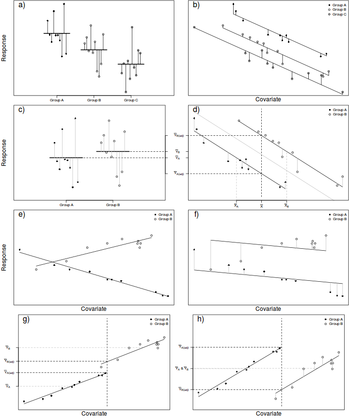
As an example, an experiment might be set up to investigate the energetic impacts of sexual vs parthenogenetic (egg development without fertilization) reproduction on leaf insect food consumption. To do so, researchers could measure the daily food intake of individual adult female leaf insects from female only (parthenogenetic) and mixed (sexual) populations. Unfortunately, the available individual leaf insects varied substantially in body size which was expected to increase the variability of daily food intake of treatment groups. Consequently, the researchers also measured the body mass of the individuals as a covariate, thereby providing a means by which daily food consumption could be standardized for body mass.
Although ANCOVA and blocking designs both aim to reduce the sources of unexplained variation by incorporating additional variables, blocking designs do so by measuring a response to each level of a treatment factor under a similar (standardized) set of unmeasured conditions. By contrast, ANCOVA attempts to reduce unexplained variability by standardizing the response to the treatment by the effects of the specific covariate condition.
Thus ANCOVA provides a means of exercising some statistical control over the variability when it is either not possible or not desirable to exercise experimental control (such as blocking or using otherwise homogeneous observations). From the example above, the researchers decided that the experiment would be too drawn out if each individual were to be measured under both sexual and parthenogenetic situations (due to the need to establish the new populations and allow enough time to minimize the risks of carryover effects).
Null hypotheses
Factor A - the main treatment effect
H$_0(A)$: $\mu_{1(adj)}=\mu_{2(adj)}=...=\mu_{i(adj)}=\mu_{(adj)}$ (the adjusted population group means are all equal)
The mean of population 1 adjusted for the covariate is equal to that of population 2 adjusted for the covariate and so on, and thus all population means adjusted for the covariate are equal to an overall adjusted mean.
If the effect of the $i^{th}$ group is the difference between the $i^{th}$ group adjusted mean and the overall adjusted mean ($\alpha_{i(adj)} = \mu_{i(adj)} - \mu_{(adj)}$) then the H$_0$ can alternatively be written as:
H$_0(A)$: $\alpha_{1(adj)} = \alpha_{2(adj)} = ... = \alpha_{i(adj)} = 0$ (the effect of each group equals zero)
If one or more of the $\alpha_{i(adj)}$ are different from zero (the response mean for this treatment differs from the overall response mean), the null hypothesis is not true indicating that the treatment does affect the response variable.
Factor B - the covariate effect
H$_0(B)$: $\beta_{1(pooled)}=0$ (the pooled population slope equals zero)
Note, that this null hypothesis is rarely of much interest. It is precisely because of this nuisance relationship that ANCOVA designs are applied.
Linear models
One or more covariates can be incorporated into single factor, nested, factorial and partly nested designs in order to reduce the unexplained variation. Fundamentally, the covariate(s) are purely used to adjust the response values prior to the regular analysis. The difficulty is in determining the appropriate adjustments. Following is a list of the appropriate linear models and adjusted response calculations for a range of ANCOVA designs. Note that these linear models do not include interactions involving the covariates as these are assumed to be zero. The inclusion of these interaction terms is a useful means of testing the homogeneity of slopes assumption (see )
Single categorical and single covariate
Linear model: $y_{ij}=\mu+\alpha_i + \beta(x_{ij}-\bar{x}) + \varepsilon_{ij}$
Adjustments: $y_{ij(adj)}=y_{ij}-b(x_{ij}-\bar{x})$
Linear model: $y_{ij}=\mu+\alpha_i + \beta_{YX}(x_{ij}-\bar{x}) + \beta_{YZ}(z_{ij}-\bar{z}) + \varepsilon_{ij}$
Adjustments: $y_{ij(adj)}=y_{ij}-b_{YX}(x_{ij}-\bar{x})-b_{YZ}(z_{ij}-\bar{z})$
Special attention must be paid to the issues raised for multiple linear regression (see ).
Linear model: $y_{ijk}=\mu+\alpha_i + \gamma_j + (\alpha\gamma)_{ij} + \beta(x_{ijk}-\bar{x}) +\varepsilon_{ijkl}$
Adjustments: $y_{ijk(adj)}=y_{ijk}-b(x_{ijk}-\bar{x})$
where $\beta$ is the population slope between the response and the covariate.
Linear model: $y_{ijk}=\mu+\alpha_i + \gamma_{j(i)} + \beta(x_{ijk}-\bar{x}) +\varepsilon_{ijk}$
Adjustments: $y_{ijk(adj)}=y_{ijk}-b(x_{ijk}-\bar{x})$
Linear model: $y_{ijkl}=\mu+\alpha_i + \gamma_{j(i)} + \delta_k + (\alpha\delta)_{ik} + \gamma\delta_{j(i)k} + \beta(x_{ijk}-\bar{x}) +\varepsilon_{ijkl}$
Adjustments: $y_{ijk(adj)}=y_{ijk}-b_{between}(x_{i}-\bar{x})-b_{within}(x_{ijk}-\bar{x}_i)$
where $b_{between}$ and $b_{within}$ refer to the between and within block/plot/subject regression slopes respectively.
Analysis of Variance
In ANCOVA, the total variability of the response variable is sequentially partitioned into components explained by each of the model terms, starting with the covariate and is therefore equivalent to performing a regular analysis of variance on the response variables that have been adjusted for the covariate. The appropriate unexplained residuals and therefore the appropriate \textit{F}-ratios for each factor differ according to the different null hypotheses associated with different linear models as well as combinations of fixed and random factors in the model (see the following tables). Note that since the covariate levels measured are typically different for each group, ANCOVA designs are inherently non-orthogonal (unbalanced). Consequently, sequential (Type I sums of squares) should not be used. {For very simple Ancova designs that incorporate a single categorical and single covariate, Type I sums of squares can be used provided the covariate appears in the linear model first (and thus is partitioned out last) as we are typically not interested in estimating this effect.
A, categorical, B continuous covariate| F-ratio | ||||
|---|---|---|---|---|
| Factor | d.f. | MS | A&B fixed | A random, B fixed |
| A | $a-1$ | $MS_{A}$ | $\frac{MS_{A}}{MS_{Resid}}$ | $\frac{MS_{A}}{MS_{Resid}}$ |
| B | $1$ | $MS_{B}$ | $\frac{MS_{B}}{MS_{Resid}}$ | $[\frac{MS_{B}}{MS_{Resid}}]$ |
| BxA | $a-1$ | $MS_{BxA}$ | $\frac{MS_{BxA}}{MS_{Resid}}$ | $\frac{MS_{BxA'}}{MS_{Resid}}$ |
| Residual (=N$^\prime$(BxA)) | $(n-2)a$ | $MS_{Resid}$ | ||
anova(lm(DV ~ B * A, dataset)) # OR anova(aov(DV ~ B * A, dataset)) # OR (make sure not using treatment contrasts) Anova(lm(DV ~ B * A, dataset), type = "III") |
||||
A and B categorical, C continuous covariate
| F-ratio | |||||
|---|---|---|---|---|---|
| Factor | d.f. | MS | A&B fixed | A random, B fixed | A&B random |
| A | $a-1$ | $MS_{A}$ | $\frac{MS_{A}}{MS_{Resid}}$ | $[\frac{MS_{A'}}{MS_{B'\times A}}]$ | $[\frac{MS_{A'}}{MS_{B'\times A'}}]$ |
| B | $b-1$ | $MS_{B}$ | $\frac{MS_{B}}{MS_{Resid}}$ | $[\frac{MS_{B'}}{MS_{Resid}}]$ | $[\frac{MS_{B'}}{MS_{B'\times A'}}]$ |
| BxA | $(b-1)(a-1)$ | $MS_{BxA}$ | $\frac{MS_{BxA}}{MS_{Resid}}$ | $\frac{MS_{B'\times A}}{MS_{Resid}}$ | $\frac{MS_{B'\times A'}}{MS_{Resid}}$ |
| C | $1$ | $MS_{C}$ | $\frac{MS_{C}}{MS_{Resid}}$ | $[\frac{MS_{C}}{MS_{C\times A'}}]$ | $[\frac{MS_{C}}{MS_{C\times A'} + MS_{C\times B'} + MS_{C\times B'\times A'}}]$ |
| CxA | $a-1$ | $MS_{C\times A}$ | $\frac{MS_{C\times A}}{MS_{Resid}}$ | $[\frac{MS_{C\times A}}{MS_{C\times B'\times A}}]$ | $[\frac{MS_{C\times A}}{MS_{C\times B'\times A'}}]$ |
| CxB | $b-1$ | $MS_{C\times B}$ | $\frac{MS_{C\times B}}{MS_{Resid}}$ | $[\frac{MS_{C\times B'}}{MS_{Resid}}]$ | $[\frac{MS_{C\times B'}}{MS_{C\times B'\times A'}}]$ |
| CxBxA | $(b-1)(a-1)$ | $MS_{C\times B\times A}$ | $\frac{MS_{C\times B\times A}}{MS_{Resid}}$ | $[\frac{MS_{C\times B'\times A}}{MS_{Resid}}]$ | $[\frac{MS_{C\times B'\times A'}}{MS_{Resid}}]$ |
| Residual (=N$^\prime$(CxBxA)) | $(n-2)ba$ | $MS_{Resid}$ | |||
anova(lm(DV ~ C * B * A, dataset)) # OR anova(aov(DV ~ C * B * A, dataset)) # OR (make sure not using treatment contrasts) Anova(lm(DV ~ C * B * A, dataset), type = "III") |
|||||
Assumptions
As ANCOVA designs are essentially regular ANOVA designs that are first adjusted (centered) for the covariate(s), ANCOVA designs inherit all of the underlying assumptions of the appropriate ANOVA design. Readers should also eventually consult Tutorial 7.6a, Tutorial 9.2a, Tutorial 9.3a and Tutorial 9.4a. Specifically, hypothesis tests assume that:
- the appropriate residuals are normally distributed. Boxplots using the appropriate scale of replication (reflecting the appropriate residuals/F-ratio denominator, see the above tables) should be used to explore normality. Scale transformations are often useful.
- the appropriate residuals are equally varied. Boxplots and plots of means against variance (using the appropriate scale of replication) should be used to explore the spread of values. Residual plots should reveal no patterns. Scale transformations are often useful.
- the appropriate residuals are independent of one another.
- the relationship between the response variable and the covariate should be linear. Linearity can be explored using scatterplots and residual plots should reveal no patterns.
- for repeated measures and other designs in which treatment levels within blocks can not be be randomly ordered, the variance/covariance matrix is assumed to display sphericity.
- for designs that utilize blocking, it is assumed that there are no block by within block interactions
Homogeneity of Slopes
In addition to the above assumptions, ANCOVA designs also assume that slopes of relationships between the response variable and the covariate(s) are the same for each treatment level (group). That is, all the trends are parallel. If the individual slopes deviate substantially from each other (and thus the overall slope), then adjustments made to each of the observations are nonsensical (see Figures e-f above). This situation is analogous to an interaction between two or more factors. In ANCOVA, interactions involving the covariate suggest that the nature of the relationship between the response and the covariate differs between the levels of the categorical treatment. More importantly, they also indicate that whether or not there is an effect of the treatment depends on what range of the covariate you are focussed on. Clearly then, it is not possible to make conclusions about the main effects of treatments in the presence of such interactions. The assumption of homogeneity of slopes can be examined via interaction plots or more formally, by testing hypotheses about the interactions between categorical variables and the covariate(s).
There are three broad approaches for dealing with ANCOVA designs with heterogeneous slopes and selection depends on the primary focus of the study.
- When the primary objective of the analysis is to investigate the effects of categorical treatments, it is possible to adopt an approach similar to that taken when exploring interactions in multiple regression. The effect of treatments can be examined at specific values of the covariate (such as the mean and $\pm$ one standard deviation). This approach is really only useful at revealing broad shifts in patterns over the range of the covariate and if the selected values of the covariate do not have some inherent biological meaning (selected arbitrarily), then the outcomes can be of only limited biological interest.
- Alternatively, the Johnson-Neyman technique (or Wilxon modification thereof) procedure indicates the ranges of the covariate over which the individual regression lines of pairs of treatment groups overlap or cross. Although less powerful than the previous approach, the Wilcox(J-N) procedure has the advantage of revealing the important range (ranges for which the groups are different and not different) of the covariate rather than being constrained by specific levels selected.
- Use contrast treatments to split up the interaction term into its constituent contrasts for each level of the treatment. Essentially this compares each of the treatment level slopes to the slope from the 'control' group and is useful if the primary focus is on the relationships between the response and the covariate
Similar covariate ranges
Adjustments made to the response means in an attempt to statistically account for differences in the covariate involve predicting mean response values along displaced linear relationships between the overall response and covariate variables (see Figure d above). The degree of trend displacement for any given group is essentially calculated by multiplying the overall regression slope by the degree of difference between the overall covariate mean and the mean of the covariate for that group. However, when the ranges of the covariate within each of the groups differ substantially from one another, these adjustments are effectively extrapolations (see Figures g-h above) and therefore of unknown reliability. If a simple ANOVA of the covariate modelled against the categorical factor indicates that the covariate means differ significantly between groups, it may be necessary to either remove extreme observations or reconsider the analysis.
Robust ANCOVA
ANCOVA based on rank transformed data can be useful for accommodating data with numerous problematic outliers. Nevertheless, the problems highlighted in section Tutorial 7.6a, Ranks about the difficulties of detecting interactions from rank transformed data obviously have implications for inferential tests of homogeneity of slopes. Randomization tests that maintain response-covariate pairs and repeatedly randomize these observations amongst the levels of the treatments can also be useful, particularly when there is doubt over the independence of observations.
Specific comparisons
Both planned and unplanned comparisons follow those of other ANOVA chapters without any real additional complications. Notably, recent implementations of the Tukey's test (within R) accommodate unbalanced designs and thus negate the need for some of the more complicated and specialized techniques that have been highlighted in past texts.
ANCOVA in R
Data and scenario
Consider an experimental design aimed at exploring the effects of a categorical variable with three levels (Group A, Group B and Group C) on a response. From previous studies, we know that the response is influenced by another variable (covariate). Unfortunately, it was not possible to ensure that all sampling units were the same degree of the covariate. Therefore, in an attempt to account for this anticipated extra source of variability, we measured the level of the covariate for each sampling unit. Actually, in allocating treatments to the various treatment groups, we tried to ensure a similar mean and range of the covariate within each group.
- the sample size per treatment=10
- the categorical $x$ variable with 3 levels
- the first treatment group has a population mean of 40.
- the other two treatments reduce the mean by 15 and 20 units respectively
- the data are drawn from normal distributions with a mean of 0 and standard deviation of 4 ($\sigma^2=16$)
- the covariate (B) is a continuous variable with a mean of 20 and a standard deviation of 15
set.seed(3)
n <- 10
p <- 3
A.eff <- c(40, -15, -20)
beta <- -0.45
sigma <- 4
B <- rnorm(n * p, 0, 15)
A <- gl(p, n, lab = paste("Group", LETTERS[1:3]))
mm <- model.matrix(~A + B)
data <- data.frame(A = A, B = B, Y = as.numeric(c(A.eff, beta) %*% t(mm)) + rnorm(n * p, 0, 4))
data$B <- data$B + 20
head(data)
        A         B        Y
1 Group A  5.570999 50.09555
2 Group A 15.612114 45.38163
3 Group A 23.881823 41.16404
4 Group A  2.718022 50.72290
5 Group A 22.936742 37.26995
6 Group A 20.451859 42.61873
Exploratory data analysis
library(car)
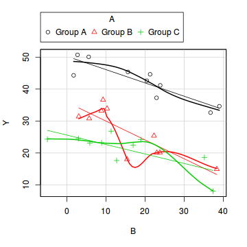
scatterplot(Y ~ B | A, data = data)
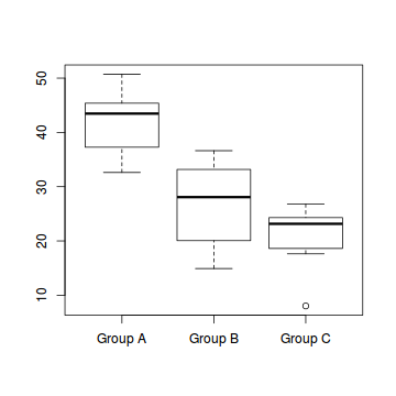
boxplot(Y ~ A, data)
# OR via ggplot
library(ggplot2)
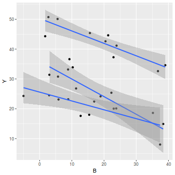
ggplot(data, aes(y = Y, x = B, group = A)) + geom_point() + geom_smooth(method = "lm")
ggplot(data, aes(y = Y, x = A)) + geom_boxplot()
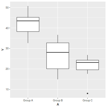
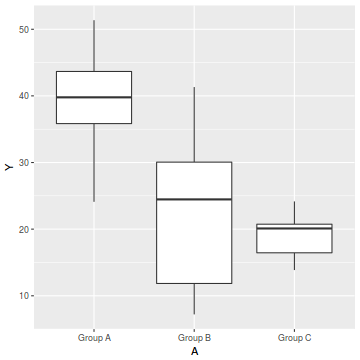
- there is no evidence of obvious non-normality
- the assumption of linearity seems reasonable
- the variability of the three groups seems approximately equal
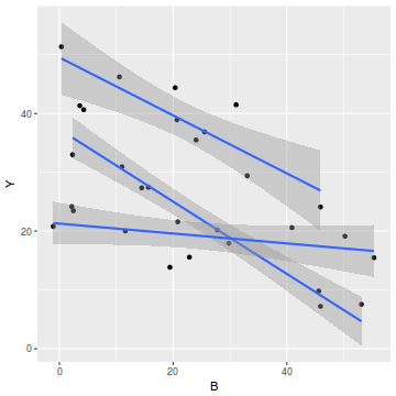
- the slopes (Y vs B trends) appear broadly similar for each treatment group
Homogeneity of slopes
We can explore inferential evidence of unequal slopes by examining estimated effects of the interaction between the categorical variable and the covariate. Note, pay no attention to the main effects - only the interaction.
anova(lm(Y ~ B * A, data = data))
Analysis of Variance Table

Response: Y
          Df  Sum Sq Mean Sq F value    Pr(>F)
B          1  354.80  354.80 23.9691 5.414e-05 ***
A          2 2772.56 1386.28 93.6531 4.609e-12 ***
B:A        2   55.08   27.54  1.8606    0.1773
Residuals 24  355.26   14.80
---
Signif. codes:  0 '***' 0.001 '**' 0.01 '*' 0.05 '.' 0.1 ' ' 1
Model fitting or statistical analysis
In R, simple ANOVA models (being regression models) are fit using the lm() function. The most important (=commonly used) parameters/arguments for simple regression are:
- formula: the linear model relating the response variable to the linear predictor
- data: the data frame containing the data
# if not intending to look at the effect of B at all
data.lm <- lm(Y ~ B + A, data = data)
# otherwise, in order to use type III sums of squares
contrasts(data$A) <- contr.sum
data.lm1 <- lm(Y ~ B + A, data = data)
Model evaluation
Prior to exploring the model parameters, it is prudent to confirm that the model did indeed fit the assumptions and was an appropriate fit to the data. Since ANCOVA models are multiple regression models, similar diagnostics (residual plots, Cooks' D and leverage) are appropriate
Residuals
plot(data.lm)
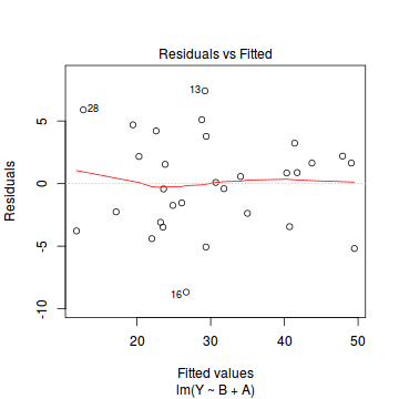
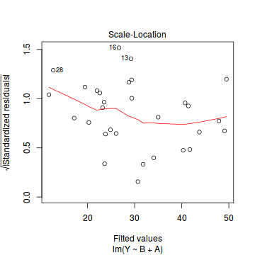
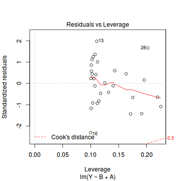
- there are no obvious patterns in the residuals (first plot). Specifically, there is no obvious 'wedge-shape' suggesting that we still have no evidence of non-homogeneity of variance
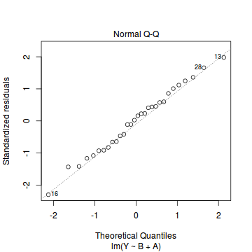
- there is no evidence of non-normality based on the Q-Q normal plot
- there are no obviously large (or small) residual or leverage values and non of the points approach the Cook's D contour of 1. Hence we can conclude that non of the observations are overly influential
Extractor functions
There are a number of extractor functions (functions that extract or derive specific information from a model) available including:| Extractor | Description |
|---|---|
| residuals() | Extracts the residuals from the model |
| fitted() | Extracts the predicted (expected) response values (on the link scale) at the observed levels of the linear predictor |
| predict() | Extracts the predicted (expected) response values (on either the link, response or terms (linear predictor) scale) |
| coef() | Extracts the model coefficients |
| confint() | Calculate confidence intervals for the model coefficients |
| summary() | Summarizes the important output and characteristics of the model |
| anova() | Computes an analysis of variance (variance partitioning) from the model |
| plot() | Generates a series of diagnostic plots from the model |
| effect() | effects package - estimates the marginal (partial) effects of a factor (useful for plotting) |
| avPlot() | car package - generates partial regression plots |
| AIC() | Compute the Akaike Information Criterion |
Exploring the model parameters, test hypotheses
If there was any evidence that the assumptions had been violated, then we would need to reconsider the model and start the process again. In this case, there is no evidence that the test will be unreliable so we can proceed to explore the test statistics.
There are two broad hypothesis testing perspectives we could take:
- We could explore the individual effects. By default, the lm() function
dummy codes the categorical variable for treatment contrasts (where each of the groups are compared to the first group).
summary(data.lm)
Call:
lm(formula = Y ~ B + A, data = data)

Residuals:
   Min     1Q Median     3Q    Max
-8.671 -2.911  0.328  2.188  7.407

Coefficients:
             Estimate Std. Error t value Pr(>|t|)
(Intercept)  50.20598    1.71450  29.283  < 2e-16 ***
B            -0.41403    0.06143  -6.740 3.76e-07 ***
AGroup B    -17.15033    1.78618  -9.602 4.91e-10 ***
AGroup C    -22.91188    1.79775 -12.745 1.09e-12 ***
---
Signif. codes:  0 '***' 0.001 '**' 0.01 '*' 0.05 '.' 0.1 ' ' 1

Residual standard error: 3.973 on 26 degrees of freedom
Multiple R-squared:  0.884,	Adjusted R-squared:  0.8706
F-statistic: 66.05 on 3 and 26 DF,  p-value: 2.719e-12
Conclusions:
- The row in the Coefficients table labeled (Intercept)
represents the first treatment group when B is equal to zero. So the Estimate for this
row represents the estimated population mean for the first treatment group (A) when B=0.
So the mean of population A is estimated to be
50.206with a standard error (precision) of1.715. Note that the rest of the columns (t value and Pr(>|t|))represent the outcome of hypothesis tests. For the first row, this hypothesis test has very little meaning as it is testing the null hypothesis that the mean of population A is zero. - The row starting with B indicates the slope of the relationship (!--rinline round(summary(data.lm)$coef[2,1],3) -->) between Y and B for the first treatment group. Recall that we must assume equal slopes for this estimate of slope (as well as the estimates of treatment effects to be appropriate).
- Each of the subsequent rows represent the estimated effects of each of the other populations from Group A.
For example, the Estimate for the row labeled AGroup B represents the estimated difference in means
between group B (for factor A) and the reference group (group A). Hence, the population mean of group B is estimated to be
17.15units lower (since has a negative sign) than the mean of group B and this 'effect' is statistically significant (at the 0.05 level). - The $R^2$ value is
0.88suggesting that approximately88% of the total variance in $Y$ can be explained by the groupings of $A$. The $R^2$ value is thus a measure of the strength of the relationship.
Alternatively, we could calculate the 95% confidence intervals for the parameter estimates.
confint(data.lm)
                  2.5 %     97.5 %
(Intercept)  46.6817751  53.730194
B            -0.5402983  -0.287754
AGroup B    -20.8218702 -13.478782
AGroup C    -26.6072038 -19.216547
- The row in the Coefficients table labeled (Intercept)
represents the first treatment group when B is equal to zero. So the Estimate for this
row represents the estimated population mean for the first treatment group (A) when B=0.
So the mean of population A is estimated to be
-
In addition (or alternatively), we could explore the collective null hypothesis (that all the population means are equal)
by partitioning the variance into explained and unexplained components (in an ANOVA table).
anova(data.lm)
Analysis of Variance Table

Response: Y
          Df  Sum Sq Mean Sq F value    Pr(>F)
B          1  354.80  354.80  22.481 6.651e-05 ***
A          2 2772.56 1386.28  87.838 2.717e-12 ***
Residuals 26  410.34   15.78
---
Signif. codes:  0 '***' 0.001 '**' 0.01 '*' 0.05 '.' 0.1 ' ' 1
# OR with type III sums of squares library(car) Anova(data.lm, type = "III")
Anova Table (Type III tests)

Response: Y
             Sum Sq Df F value    Pr(>F)
(Intercept) 13533.2  1 857.502 < 2.2e-16 ***
B             716.9  1  45.424 3.756e-07 ***
A            2772.6  2  87.838 2.717e-12 ***
Residuals     410.3 26
---
Signif. codes:  0 '***' 0.001 '**' 0.01 '*' 0.05 '.' 0.1 ' ' 1
Conclusions:
- The ratio of mean variance explained by the main effect (A) to mean unexplained variance is
NA- which is substantially higher than what would be expected if the null hypothesis was true. We would reject the null hypothesis that all the population means are equal ($p<0.05$). At least one of the populations is different from the others. - Overall, there is an effect of treatment on the response.
- Note that the first ANOVA has underestimated the effect of the covariate (B) due to the inherently unbalanced nature of the design. If we are not interested in estimating the magnitude of this effect (as is often the case if B is just a covariate added to soak up some unexplained variance), we can ignore this. Note that the effect of interest should be the last term in the model to ensure it is estimated correctlyI. f however, we require an estimate of each effect, then type III Sums of Squares should be used.
- The ratio of mean variance explained by the main effect (A) to mean unexplained variance is
Predictions
As with other regressions, we can predict new responses. In the case of the ANCOVA as described above (where B is added purely to soak up noise and does not require estimating), we would probably like to predict values associated with the three levels of the main treatment effect at the average level of the covariate.
predict(data.lm, newdata = data.frame(A = levels(data$A), B = mean(data$B, na.rm = TRUE)), interval = "prediction")
       fit      lwr      upr
1 43.37383 34.80352 51.94413
2 26.22350 17.65873 34.78827
3 20.46195 11.89377 29.03013
Prediction intervals represent the intervals associated with predicting any single new observation. Confidence intervals on the other hand, represent intervals associated with the estimated means. In essence the are the confidence in a mean of values rather than a single value. Consequently, confidence intervals are narrower than prediction intervals.
Note that confidence intervals of each population can alternatively have been achieved by fitting a means model and calculating the confidence intervals for the parameter estimates.
predict(data.lm, newdata = data.frame(A = levels(data$A), B = mean(data$B, na.rm = TRUE)), interval = "confidence")
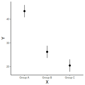
       fit      lwr      upr
1 43.37383 40.77244 45.97522
2 26.22350 23.64040 28.80661
3 20.46195 17.86757 23.05634
Graphical Summaries
Effects plots
Effects plots display the modeled effects
library(effects)
plot(effect("A", data.lm))
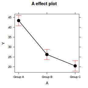
plot(effect("B", data.lm, partial.residuals = TRUE))
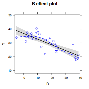
plot(allEffects(data.lm, partial.residuals = TRUE))
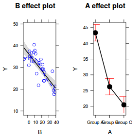
Obviously we could also roll our own.
## generate a prediction data frame
newdata <- data.frame(A = levels(data$A), B = mean(data$B, na.rm = TRUE))
fit <- predict(data.lm, newdata = newdata, interval = "confidence")
fit <- data.frame(newdata, fit)

library(ggplot2)
ggplot(fit, aes(y = fit, x = A)) + geom_pointrange(aes(ymin = lwr, ymax = upr)) +
    scale_y_continuous("Y") + scale_x_discrete("X") + theme_classic() +
    theme(axis.title.y = element_text(vjust = 1, size = rel(1.25)), axis.title.x = element_text(vjust = -1,
        size = rel(1.25)))
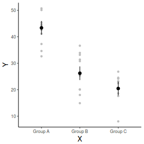
And if we wished to add the observed values to this figure.
library(ggplot2)
ggplot(fit, aes(y = fit, x = A)) + geom_point(data = data, aes(y = Y),
    col = "grey") + geom_pointrange(aes(ymin = lwr, ymax = upr)) + scale_y_continuous("Y") +
    scale_x_discrete("X") + theme_classic() + theme(axis.title.y = element_text(vjust = 1,
    size = rel(1.25)), axis.title.x = element_text(vjust = -1, size = rel(1.25)))
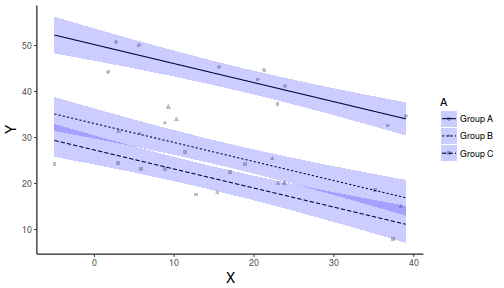
And if we wanted to show the separate trends per group
library(ggplot2)
newdata <- expand.grid(A = levels(data$A), B = seq(min(data$B), max(data$B),
    l = 10))
fit <- predict(data.lm, newdata = newdata, interval = "confidence")
fit <- data.frame(newdata, fit)
part.obs <- cbind(data, part.obs = fitted(data.lm) + resid(data.lm))
ggplot(fit, aes(y = fit, x = B, group = A, linetype = A)) + geom_point(data = part.obs,
    aes(y = part.obs, shape = A), col = "grey") + geom_line() + geom_ribbon(aes(ymin = lwr,
    ymax = upr), fill = "blue", alpha = 0.2) + scale_y_continuous("Y") +
    scale_x_continuous("X") + theme_classic() + theme(axis.title.y = element_text(vjust = 1,
    size = rel(1.25)), axis.title.x = element_text(vjust = -1, size = rel(1.25)))
Dealing with heterogeneous slopes
- the sample size per treatment=10
- the categorical $x$ variable with 3 levels
- the first treatment group has a population mean of 40.
- the other two treatments reduce the mean by 15 and 20 units respectively
- the data are drawn from normal distributions with a mean of 0 and standard deviation of 4 ($\sigma^2=16$)
- the covariate (B) is a continuous variable with a mean of 20 and a standard deviation of 15
set.seed(6)
n <- 10
p <- 3
A.eff <- c(40, -15, -20)
beta <- c(-0.45, -0.1, 0.5)
sigma <- 4
B <- rnorm(n * p, 0, 15)
A <- gl(p, n, lab = paste("Group", LETTERS[1:3]))
mm <- model.matrix(~A * B)
data1 <- data.frame(A = A, B = B, Y = as.numeric(c(A.eff, beta) %*% t(mm)) + rnorm(n * p, 0, 4))
data1$B <- data1$B + 20
head(data1)
        A        B        Y
1 Group A 24.04409 35.49432
2 Group A 10.55022 46.22216
3 Group A 33.02990 29.41898
4 Group A 45.90793 24.10656
5 Group A 20.36281 44.38834
6 Group A 25.52038 36.87477
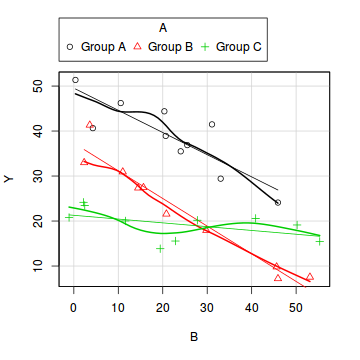
Exploratory data analysis
        library(car)
        scatterplot(Y~B|A, data=data1)
boxplot(Y~A, data1)
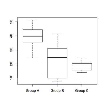
        #OR via ggplot
        library(ggplot2)
        ggplot(data1, aes(y=Y, x=B, group=A)) + geom_point() + geom_smooth(method='lm')
ggplot(data1, aes(y=Y, x=A)) + geom_boxplot()
Homogeneity of slopes
We can explore inferential evidence of unequal slopes by examining estimated effects of the interaction between the categorical variable and the covariate. Note, pay no attention to the main effects - only the interaction.
anova(lm(Y ~ B * A, data = data1))
Analysis of Variance Table

Response: Y
          Df  Sum Sq Mean Sq F value    Pr(>F)
B          1 1257.14 1257.14  98.520 5.685e-10 ***
A          2 2042.02 1021.01  80.015 2.420e-11 ***
B:A        2  510.02  255.01  19.985 7.778e-06 ***
Residuals 24  306.25   12.76
---
Signif. codes:  0 '***' 0.001 '**' 0.01 '*' 0.05 '.' 0.1 ' ' 1
Model fitting or statistical analysis
Since there is strong evidence of an interaction (non-homogeneous slopes) we cannot fit a simple ANCOVA model. We do however have a couple of options:
- examine the effect of the categorical variable at specific levels of the covariate
data1.lm <- lm(Y ~ B * A, data = data1)
library(contrast)
contrast(data1.lm, a = list(A = "Group B", B = mean(data1$B) - 2 * sd(data1$B)), b = list(A = "Group C",
    B = mean(data1$B) - 2 * sd(data1$B)))
lm model parameter contrast

 Contrast     S.E.    Lower    Upper    t df Pr(>|t|)
 22.00042 3.448672 14.88271 29.11813 6.38 24        0
contrast(data1.lm, a = list(A = "Group B", B = mean(data1$B) - sd(data1$B)), b = list(A = "Group C",
    B = mean(data1$B) - sd(data1$B)))
lm model parameter contrast

 Contrast     S.E.    Lower    Upper    t df Pr(>|t|)
 12.91806 2.234074 8.307162 17.52897 5.78 24        0
contrast(data1.lm, a = list(A = "Group B", B = mean(data1$B)), b = list(A = "Group C", B = mean(data1$B)))
lm model parameter contrast

 Contrast     S.E.     Lower    Upper   t df Pr(>|t|)
 3.835712 1.599551 0.5344006 7.137024 2.4 24   0.0246
contrast(data1.lm, a = list(A = "Group B", B = mean(data1$B) + sd(data1$B)), b = list(A = "Group C",
    B = mean(data1$B) + sd(data1$B)))
lm model parameter contrast

  Contrast     S.E.     Lower      Upper     t df Pr(>|t|)
 -5.246639 2.143777 -9.671177 -0.8221018 -2.45 24   0.0221
contrast(data1.lm, a = list(A = "Group B", B = mean(data1$B) + 2 * sd(data1$B)), b = list(A = "Group C",
    B = mean(data1$B) + 2 * sd(data1$B)))
lm model parameter contrast

  Contrast     S.E.     Lower     Upper    t df Pr(>|t|)
 -14.32899 3.332076 -21.20606 -7.451925 -4.3 24    2e-04
- apply the Wilcox modification of the Johnsone-Neyman technique to explore the ranges of the covariate over which treatment groups are different.
Conclusions:
## The following are used for the Johnson-Neyman Wilcox procedure 1. JN - is an internal 2. wilcox.JN
## - is the external
JN <- function(N1, M1, SSx1, b01, b11, SEres1, N2, M2, SSx2, b02, b12, SEres2, tmts, type = "H") {
    ## calculate the MSresiduals
    MSres1 <- SEres1/(N1 - 2)
    MSres2 <- SEres2/(N2 - 2)

    ## determine the degrees of freedom
    FNcalcD <- function(samplesize, covmean, covval, covss) {
        ## calculates the value of 'd' in the equations
        (1/samplesize) + (((covmean - covval)^2)/covss)
    }
    d1 <- FNcalcD(N1, M1, M1, SSx1)
    d2 <- FNcalcD(N2, M2, M2, SSx2)
    MSres1 <- SEres1/(N1 - 2)
    MSres2 <- SEres2/(N2 - 2)
    mu1 = MSres1 * d1
    mu2 = MSres2 * d2
    (nu <- as.integer((((mu1 + mu2)^2)/((mu1^2/(N1 - 2)) + (mu2^2/(N2 - 2))))))

    interpval <- function(lowdf, lowval, highdf, highval, compdf) {
        while (1 == 1) {
            newdf <- ((highdf - lowdf)/2) + lowdf
            newval <- 1/(0.5 * ((1/lowval) + (1/highval)))
            if (abs(newdf - compdf) < 0.1)
                break
            if (newdf > compdf) {
                highdf <- newdf
                highval <- newval
            }
            if (newdf < compdf) {
                lowdf <- newdf
                lowval <- newval
            }
        }
        newval
    }

    critvalue <- function(tmatrix, tmts, nu) {
        Hmatrix <- structure(c(4.38, 4.13, 3.97, 3.85, 3.76, 3.69, 3.64, 3.59, 3.56, 3.53, 3.49, 3.48,
            3.46, 3.44, 3.43, 3.41, 3.37, 3.33, 3.28, 3.23, 3.21, 5.38, 5.03, 4.79, 4.64, 4.52, 4.42,
            4.35, 4.29, 4.24, 4.19, 4.16, 4.12, 4.09, 4.07, 4.05, 4.03, 3.97, 3.91, 3.85, 3.78, 3.74,
            6.01, 5.59, 5.33, 5.13, 4.99, 4.88, 4.79, 4.71, 4.65, 4.59, 4.55, 4.52, 4.48, 4.45, 4.43,
            4.39, 4.33, 4.26, 4.18, 4.09, 4.05, 6.47, 6.01, 5.71, 5.49, 5.33, 5.19, 5.09, 5.02, 4.95,
            4.89, 4.84, 4.79, 4.76, 4.73, 4.69, 4.67, 4.59, 4.51, 4.42, 4.33, 4.27, 6.83, 6.34, 6.01,
            5.77, 5.59, 5.46, 5.35, 5.26, 5.19, 5.12, 5.07, 5.02, 4.98, 4.94, 4.91, 4.88, 4.79, 4.69,
            4.61, 4.51, 4.44, 7.12, 6.59, 6.25, 5.99, 5.82, 5.67, 5.55, 5.46, 5.38, 5.31, 5.25, 5.19,
            5.16, 5.12, 5.08, 5.05, 4.96, 4.86, 4.76, 4.66, 4.58, 7.37, 6.83, 6.46, 6.19, 5.99, 5.85,
            5.73, 5.63, 5.54, 5.47, 5.41, 5.36, 5.31, 5.27, 5.23, 5.19, 5.09, 4.99, 4.89, 4.78, 4.69),
            .Dim = c(21L, 7L), .Dimnames = list(c("5", "6", "7", "8", "9", "10", "11", "12", "13", "14",
                "15", "16", "17", "18", "19", "20", "24", "30", "40", "60", "120"), c("2", "3", "4",
                "5", "6", "7", "8")))
        ## matrix of H values - 1st line is data for matrix size 1st dimension of matrix is rows - degrees of
        ## freedom 2nd is cols - number of treatments 3rd - probability - currently 0.05 only
        SMMmatrix <- structure(c(5.57, 3.96, 3.38, 3.09, 2.92, 2.8, 2.72, 2.66, 2.61, 2.57, 2.54, 2.49,
            2.46, 2.43, 2.41, 2.38, 2.35, 2.32, 2.29, 2.24, 6.34, 4.43, 3.74, 3.4, 3.19, 3.06, 2.96,
            2.89, 2.83, 2.78, 2.75, 2.69, 2.65, 2.62, 2.59, 2.56, 2.52, 2.49, 2.45, 2.39, 6.89, 4.76,
            4, 3.62, 3.39, 3.24, 3.13, 3.05, 2.98, 2.93, 2.89, 2.83, 2.78, 2.75, 2.72, 2.68, 2.64, 2.6,
            2.56, 2.49, 7.31, 5.02, 4.2, 3.79, 3.54, 3.38, 3.26, 3.17, 3.1, 3.05, 3, 2.94, 2.89, 2.85,
            2.82, 2.77, 2.73, 2.69, 2.65, 2.57, 7.65, 5.23, 4.37, 3.93, 3.66, 3.49, 3.36, 3.27, 3.2,
            3.14, 3.09, 3.02, 2.97, 2.93, 2.9, 2.85, 2.8, 2.76, 2.72, 2.63), .Dim = c(20L, 5L), .Dimnames = list(c("2",
            "3", "4", "5", "6", "7", "8", "9", "10", "11", "12", "14", "16", "18", "20", "24", "30",
            "40", "60", "10000"), c("2", "3", "4", "5", "6")))
        ## matrix of SMM values - 1st line is data for matrix size 1st dimension of matrix is rows - degrees
        ## of freedom 2nd is cols - number of contrasts 3rd - probability - currently 0.05 only

        ## need to put in a catch to get number of categories greater than are in the H or SMM table
        if (tmatrix == "Hmatrix")
            hmatrix <- Hmatrix
        if (tmatrix == "SMMmatrix")
            hmatrix <- SMMmatrix
        lowval <- 0
        lowdof <- 0
        highval <- 0
        highdof <- 0
        for (i in 1:nrow(hmatrix)) {
            # print(as.numeric(rownames(hmatrix)[i])) print(nu)
            if (as.numeric(rownames(hmatrix)[i]) < nu) {
                lowdof <- as.numeric(rownames(hmatrix)[i])
                lowval <- hmatrix[i, as.character(tmts)]
            }
            if (as.numeric(rownames(hmatrix)[i]) > nu) {
                highdof <- as.numeric(rownames(hmatrix)[i])
                highval <- hmatrix[i, as.character(tmts)]
                value <- interpval(lowdof, lowval, highdof, highval, nu)
                break
            }
            if (as.numeric(rownames(hmatrix)[i]) == nu) {
                value <- hmatrix[i, as.character(tmts)]
                break
            }
        }
        class(value) <- "H"
        value
    }
    ## calculate the critical h value
    if (type == "H") {
        h <- critvalue("Hmatrix", tmts, nu)
    } else {
        h <- (2^0.5) * critvalue("SMMmatrix", tmts, nu)
    }

    A <- ((h^2)/2) * ((MSres1/SSx1) + (MSres2/SSx2))
    A <- ((b11 - b12)^2) - A
    B <- (h^2) * ((MSres1 * M1/SSx1) + (MSres2 * M2/SSx2))
    B <- B + (2 * ((b01 - b02) * (b11 - b12)))
    C <- -((h^2)/2) * ((MSres1/N1) + (MSres2/N2))
    firsthalf <- MSres1 * ((M1^2)/SSx1)
    secondhalf <- MSres2 * ((M2^2)/SSx2)
    C <- C - (((h^2)/2) * (firsthalf + secondhalf))
    C <- C + ((b01 - b02)^2)

    XLOWER <- (-B - sqrt((B^2) - (4 * A * C)))/(2 * A)
    XUPPER <- (-B + sqrt((B^2) - (4 * A * C)))/(2 * A)

    c(nu, h, XLOWER, XUPPER)
}

wilcox.JN <- function(object, type = "H") {
    NumLevels <- length(unlist(object$xlevels))
    combN <- choose(NumLevels, 2)
    combS <- combn(unlist(object$xlevels), 2)
    tab <- matrix(1, nrow = combN, ncol = 4)
    rownames(tab) <- apply(combS, 2, paste, collapse = " vs ")
    colnames(tab) <- c("df", "critical value", "lower", "upper")
    # determine the covariate
    covName <- attr(object$terms, "dataClasses")[-attr(object$terms, "response")]
    covName <- names(covName[covName != "factor"])
    for (i in 1:combN) {
        LEV1 <- combS[1, i]
        N1 <- length(object$model[2][object$model[3] == LEV1])
        M1 <- mean(object$model[2][object$model[3] == LEV1])
        SSx1 <- var(object$model[2][object$model[3] == LEV1]) * (N1 - 1)
        lmm <- eval(parse(text = paste("update(object, ~", covName, ", subset=", names(object$xlevels),
            "=='", LEV1, "')", sep = "")))
        b01 <- summary(lmm)$coef[1, 1]
        b11 <- summary(lmm)$coef[2, 1]
        SEres1 <- anova(lmm)[2, 2]
        LEV2 <- combS[2, i]
        N2 <- length(object$model[2][object$model[3] == LEV2])
        M2 <- mean(object$model[2][object$model[3] == LEV2])
        SSx2 <- var(object$model[2][object$model[3] == LEV2]) * (N2 - 1)
        lmm <- eval(parse(text = paste("update(object, ~", covName, ", subset=", names(object$xlevels),
            "=='", LEV2, "')", sep = "")))
        b02 <- summary(lmm)$coef[1, 1]
        b12 <- summary(lmm)$coef[2, 1]
        SEres2 <- anova(lmm)[2, 2]
        tab[i, ] <- (JN(N1, M1, SSx1, b01, b11, SEres1, N2, M2, SSx2, b02, b12, SEres2, NumLevels, type))
    }
    tab
}

data1.lm <- lm(Y ~ B * A, data = data1)
wilcox.JN(data1.lm)
                   df critical value    lower      upper
Group A vs Group B 13           4.24 82.18704  -6.395548
Group A vs Group C 14           4.19 45.34543 369.010466
Group B vs Group C 15           4.16 22.65381  40.450698
- the lower value of the interval (lower,upper) for the comparison of Group A and Group B is higher than the upper value. This is an artifact of the calculations and essentially signifies that the two Groups are different throughout the natural range of the covariate (B).
- for the comparison of Group A and Group C, the interval of overlap is from
45.35to369.01. Hence after a covariate value of45.35, Group A and C are not significantly different. - Group B and Group C, are not considered to be significantly different within the covariate range of
22.65to40.45
Worked Examples
- McCarthy (2007) - Chpt 6
- Kery (2010) - Chpt 10
- Gelman & Hill (2007) - Chpt 4
- Logan (2010) - Chpt 12
- Quinn & Keough (2002) - Chpt 9
Homogeneous slopes
To investigate the impacts of sexual activity on the fruitfly longevity, Partridge and Farquhar (1981), measured the longevity of male fruitflies with access to either one virgin female (potential mate), eight virgin females, one pregnant female (not a potential mate), eight pregnant females or no females. The pool of available male fruitflies varied in size and since size is known to impact longevity, the researchers also measured thorax length as a covariate.
Download Partridge1 data set| Format of partridge1.csv data file | ||||||||||||||||||||||
|---|---|---|---|---|---|---|---|---|---|---|---|---|---|---|---|---|---|---|---|---|---|---|
|
 |
Open the partridge1 data file. HINT.
partridge <- read.table("../downloads/data/partridge1.csv", header = T, sep = ",", strip.white = T)
head(partridge)
  TREATMENT THORAX LONGEV
1     Preg8   0.64     35
2     Preg8   0.68     37
3     Preg8   0.68     49
4     Preg8   0.72     46
5     Preg8   0.72     63
6     Preg8   0.76     39
- In the table below, list the assumptions of nested ANOVA along with how violations of each assumption are diagnosed and/or the risks of violations are minimized.
Assumption Diagnostic/Risk Minimization I. II. III. IV. V. -
Check the assumptions of normality and homogeneity of variances (HINT).
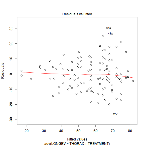
Is there any evidence of violations of the assumptions? (Y or N)
If so, assess whether a transformation will address the violations (HINT).View full codeplot(aov(LONGEV ~ THORAX + TREATMENT, partridge), which = 1)
 View full code
library(car)
scatterplot(LONGEV ~ THORAX | TREATMENT, partridge)
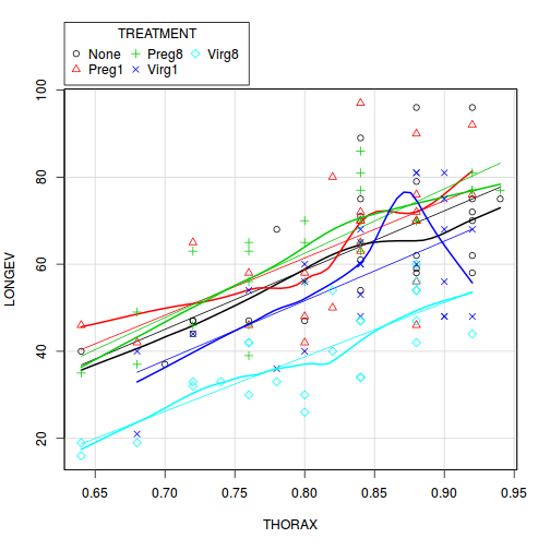 View ggplot2 code
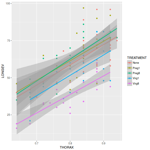
library(ggplot2)
ggplot(partridge, aes(y = LONGEV, x = THORAX, color = TREATMENT)) + geom_point() + geom_smooth(method = "lm")
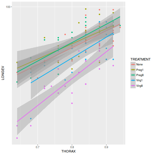
ggplot(partridge, aes(y = LONGEV, x = THORAX, color = TREATMENT)) + geom_point() + geom_smooth(method = "lm") +
    scale_y_log10()
-
Check these assumptions of linearity and homogeneity of slopes EMPIRICALLY (HINT).
Is there any evidence of violations of the assumptions? (Y or N)
View full codeanova(aov(log10(LONGEV) ~ THORAX * TREATMENT, partridge))
Analysis of Variance Table Response: log10(LONGEV) Df Sum Sq Mean Sq F value Pr(>F) THORAX 1 1.21194 1.21194 176.4955 <2e-16 *** TREATMENT 4 0.78272 0.19568 28.4970 <2e-16 *** THORAX:TREATMENT 4 0.04288 0.01072 1.5611 0.1894 Residuals 115 0.78967 0.00687 --- Signif. codes: 0 '***' 0.001 '**' 0.01 '*' 0.05 '.' 0.1 ' ' 1 - Finally,
check that the ranges of the covariate are similar for each level
of
the
categorical variable
(HINT).
Is there any evidence that the ranges of the covariate differ between the
different
levels
of
the
categorical
variable? (Y or N)
View full codeanova(aov(THORAX ~ TREATMENT, partridge))
Analysis of Variance Table Response: THORAX Df Sum Sq Mean Sq F value Pr(>F) TREATMENT 4 0.03000 0.0074992 1.2606 0.2893 Residuals 120 0.71389 0.0059491 - In addition to the global Ancova, the researchers likely
to have been interested in examining a set of specific planned
comparisons. Two such contrasts could be:
- "pregnant versus virgin partners (to investigate the impacts of any sexual activity)?" (contrast coefficients: 0, .5, .5, -.5, -.5)
- "one virgin versus eight virgin partners (to investigate the impacts of sexual frequency)?" (contrast coefficients: 0, 0, 0, 1, -1)
- Before we fit the
linear model (perform the ANOVA), we need to define the contrast
coefficients (and thus comparisons) that we wish to perform in addition
to the global ANOVA. Define
the contrasts for the TREATMENT variable
(HINT)
View full code
library(gmodels)
cmat <- make.contrasts(rbind(c(0, 0.5, 0.5, -0.5, -0.5), c(0, 0, 0, 1, -1)))
cmat
     C1   C2          C3         C4
V1  0.0  0.0 -0.38546628 -0.8071033
V2  0.5  0.0  0.73443776 -0.1029620
V3  0.5  0.0 -0.54170462  0.5065137
V4 -0.5  0.5  0.09636657  0.2017758
V5 -0.5 -0.5  0.09636657  0.2017758
round(crossprod(cmat), 1)
   C1  C2 C3 C4
C1  1 0.0  0  0
C2  0 0.5  0  0
C3  0 0.0  1  0
C4  0 0.0  0  1
contrasts(partridge$TREATMENT) <- cmat
- If there is no evidence that the assumptions have been violated and the contrasts were successfully defined, run the linear model, check residuals and examine the ANOVA table
View full code
# fit model
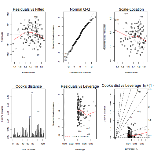
partridge.lm <- lm(log10(LONGEV) ~ THORAX + TREATMENT, partridge)

# model evaluation
par(mfrow = c(2, 3))
plot(partridge.lm, which = 1:6)
summary(partridge.lm)
Call: lm(formula = log10(LONGEV) ~ THORAX + TREATMENT, data = partridge) Residuals: Min 1Q Median 3Q Max -0.226736 -0.058445 -0.003469 0.059961 0.170389 Coefficients: Estimate Std. Error t value Pr(>|t|) (Intercept) 0.75567 0.08162 9.259 1.07e-15 *** THORAX 1.19385 0.09900 12.060 < 2e-16 *** TREATMENTC1 0.14727 0.01673 8.802 1.27e-14 *** TREATMENTC2 0.12784 0.02395 5.338 4.57e-07 *** TREATMENTC3 -0.02586 0.01674 -1.545 0.1250 TREATMENTC4 -0.03136 0.01686 -1.860 0.0654 . --- Signif. codes: 0 '***' 0.001 '**' 0.01 '*' 0.05 '.' 0.1 ' ' 1 Residual standard error: 0.08364 on 119 degrees of freedom Multiple R-squared: 0.7055, Adjusted R-squared: 0.6932 F-statistic: 57.02 on 5 and 119 DF, p-value: < 2.2e-16library(car) Anova(partridge.lm, type = "III")
Anova Table (Type III tests) Response: log10(LONGEV) Sum Sq Df F value Pr(>F) (Intercept) 0.59978 1 85.729 1.065e-15 *** THORAX 1.01749 1 145.435 < 2.2e-16 *** TREATMENT 0.78272 4 27.970 2.231e-16 *** Residuals 0.83255 119 --- Signif. codes: 0 '***' 0.001 '**' 0.01 '*' 0.05 '.' 0.1 ' ' 1summary(aov(partridge.lm), split = list(TREATMENT = list(`Preg vs Virg` = 1, `1 Virg vs * Virg` = 2)))
                               Df Sum Sq Mean Sq F value   Pr(>F)
THORAX                          1 1.2119  1.2119  173.23  < 2e-16 ***
TREATMENT                       4 0.7827  0.1957   27.97 2.23e-16 ***
  TREATMENT: Preg vs Virg       1 0.5444  0.5444   77.81 1.15e-14 ***
  TREATMENT: 1 Virg vs * Virg   1 0.1973  0.1973   28.20 5.16e-07 ***
Residuals                     119 0.8325  0.0070
---
Signif. codes:  0 '***' 0.001 '**' 0.01 '*' 0.05 '.' 0.1 ' ' 1
View full code for glslibrary(nlme) partridge.lme <- gls(log10(LONGEV) ~ THORAX + TREATMENT, partridge) anova(partridge.lme, type = "marginal")
Denom. DF: 119 numDF F-value p-value (Intercept) 1 85.72862 <.0001 THORAX 1 145.43479 <.0001 TREATMENT 4 27.96951 <.0001summary(partridge.lme)
Generalized least squares fit by REML Model: log10(LONGEV) ~ THORAX + TREATMENT Data: partridge AIC BIC logLik -222.1429 -202.689 118.0714 Coefficients: Value Std.Error t-value p-value (Intercept) 0.7556728 0.08161517 9.258975 0.0000 THORAX 1.1938527 0.09899576 12.059635 0.0000 TREATMENTC1 0.1472712 0.01673168 8.801940 0.0000 TREATMENTC2 0.1278351 0.02394896 5.337815 0.0000 TREATMENTC3 -0.0258581 0.01673758 -1.544911 0.1250 TREATMENTC4 -0.0313582 0.01686066 -1.859846 0.0654 Correlation: (Intr) THORAX TREATMENTC1 TREATMENTC2 TREATMENTC3 THORAX -0.996 TREATMENTC1 -0.019 0.019 TREATMENTC2 0.155 -0.155 -0.003 TREATMENTC3 0.032 -0.033 -0.001 0.005 TREATMENTC4 -0.124 0.125 0.002 -0.019 -0.004 Standardized residuals: Min Q1 Med Q3 Max -2.71074813 -0.69873756 -0.04147324 0.71686540 2.03709352 Residual standard error: 0.08364339 Degrees of freedom: 125 total; 119 residual - Present the results of the planned comparisons as part of the following ANOVA table:
Source of Variation SS df MS F-ratio Pvalue THORAX TREATMENT Preg vs Virg 1 Virg vs 8 Virg Residual (within groups) - How about a nice summary figure?
View full code for summary figure (ggplot2)
library(ggplot2)
library(scales)
pred <- with(partridge, expand.grid(TREATMENT = levels(TREATMENT), THORAX = seq(min(THORAX),
    max(THORAX), l = 10)))
pred <- cbind(pred, predict(partridge.lm, newdata = pred, interval = "confidence"))
br <- log10(pretty(partridge$LONGEV))
ggplot(pred, aes(y = fit, x = THORAX, linetype = TREATMENT)) + geom_point(data = partridge,
    aes(y = log10(partridge$LONGEV), shape = TREATMENT)) + geom_line() +
    geom_ribbon(aes(ymin = lwr, ymax = upr), fill = "grey", alpha = 0.2) +
    # geom_line(aes(y=lwr))+ geom_line(aes(y=upr))+
scale_y_continuous("Longevity (days)", trans = exp_trans(base = 10), breaks = br,
    labels = 10^br) + scale_x_continuous("Thorax length (mm)") + theme_classic() +
    theme(legend.position = c(1, 0), legend.justification = c(1, 0), axis.title.y = element_text(vjust = 2,
        size = rel(1.25)), axis.title.x = element_text(vjust = -2, size = rel(1.25)),
        plot.margin = unit(c(0.5, 0.5, 2, 2), "lines"))
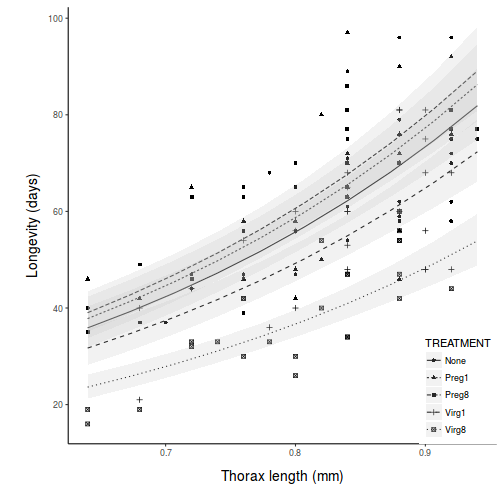
Fit the linear model and produce an ANOVA table to test the null hypotheses that there no effects of treatment (female type) on the (log transformed) longevity of male fruitflies adjusted for thorax length. Note that as the design is inherently imbalanced (since there is a different series of thorax lengths within each treatment type), Type I sums of squares are inappropriate. Therefore Type III sums of squares will be used.
Heterogeneous slopes
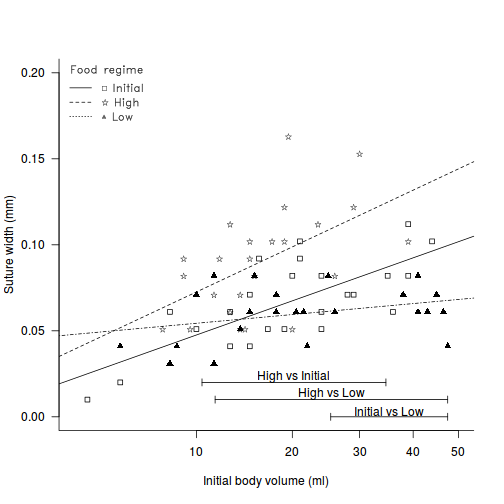
Constable (1993) compared the inter-radial suture widths of urchins maintained on one of three food regimes (Initial: no additional food supplied above what was in the initial sample, low: food supplied periodically and high: food supplied ad libitum. In an attempt to control for substantial variability in urchin sizes, the initial body volume of each urchin was measured as a covariate.
Download Constable data set| Format of constable.csv data file | ||||||||||||||||||||||
|---|---|---|---|---|---|---|---|---|---|---|---|---|---|---|---|---|---|---|---|---|---|---|
|
 |
Open the constable data file. HINT.
constable <- read.table("../downloads/data/constable.csv", header = T, sep = ",", strip.white = T)
head(constable)
    TREAT   IV  SUTW
1 Initial  3.5 0.010
2 Initial  5.0 0.020
3 Initial  8.0 0.061
4 Initial 10.0 0.051
5 Initial 13.0 0.041
6 Initial 13.0 0.061
-
In the table below, list the assumptions of nested ANOVA along with how violations of each assumption are diagnosed and/or the risks of violations are minimized.
Assumption Diagnostic/Risk Minimization I. II. III. IV. V. -
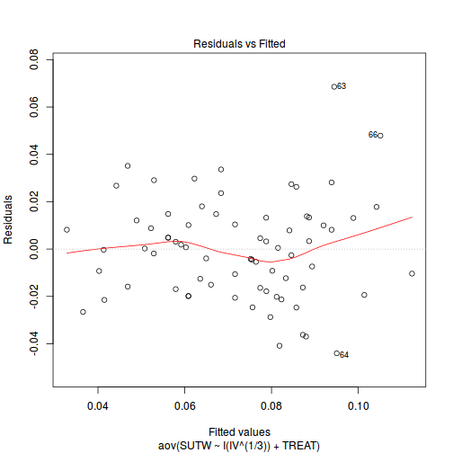
Check the assumptions of normality and homogeneity of variances (HINT).
Is there any evidence of violations of the assumptions? (Y or N) View full code
plot(aov(SUTW ~ I(IV^(1/3)) + TREAT, constable), which = 1)
-
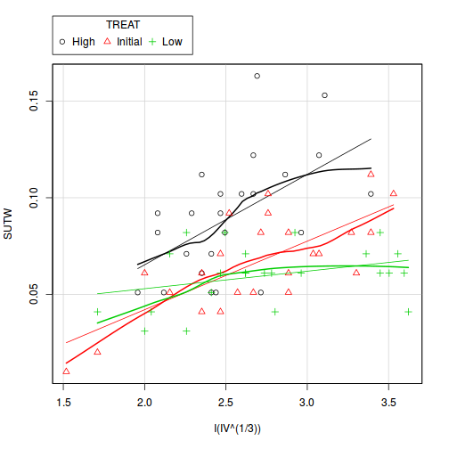
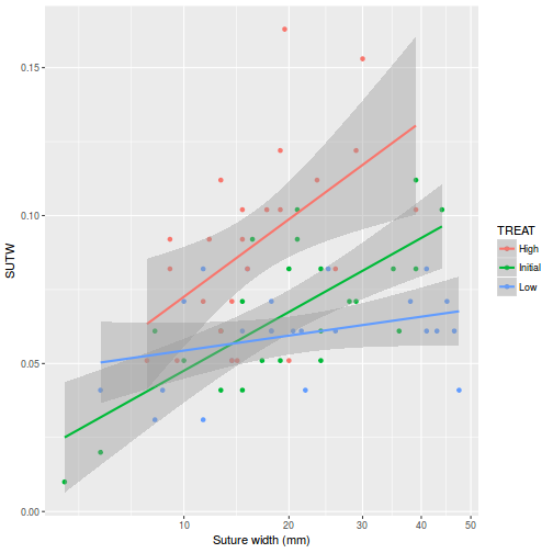
Check these assumptions of linearity and homogeneity of slopes GRAPHICALLY (HINT).
Is there any evidence of violations of the assumptions? (Y or N) View full code
library(car)
scatterplot(SUTW ~ I(IV^(1/3)) | TREAT, constable)
 View ggplot2 code
library(ggplot2)
ggplot(constable, aes(y = SUTW, x = IV, color = TREAT)) + geom_point() + geom_smooth(method = "lm") +
    scale_x_continuous("Suture width (mm)", trans = trans_new("root", function(x) x^(1/3), function(x) x^3,
        domain = c(0, Inf)))
-
Check these assumptions of linearity and homogeneity of slopes EMPIRICALLY (HINT).
Is there any evidence of violations of the assumptions? (Y or N) View full code
anova(aov(SUTW ~ I(IV^(1/3)) * TREAT, constable))
Analysis of Variance Table Response: SUTW Df Sum Sq Mean Sq F value Pr(>F) I(IV^(1/3)) 1 0.0065364 0.0065364 15.5799 0.0001945 *** TREAT 2 0.0167503 0.0083752 19.9626 1.66e-07 *** I(IV^(1/3)):TREAT 2 0.0039443 0.0019721 4.7007 0.0123436 * Residuals 66 0.0276899 0.0004195 --- Signif. codes: 0 '***' 0.001 '**' 0.01 '*' 0.05 '.' 0.1 ' ' 1 -
Finally,
check that the ranges of the covariate are similar for each level
of
the
categorical variable
(HINT).
Is there any evidence that the ranges of the covariate differ between the
different
levels
of
the
categorical
variable? (Y or N) View full code
anova(aov(I(IV^(1/3)) ~ TREAT, constable))
Analysis of Variance Table Response: I(IV^(1/3)) Df Sum Sq Mean Sq F value Pr(>F) TREAT 2 0.6556 0.32782 1.3634 0.2626 Residuals 69 16.5908 0.24045 -
Determine the regions of difference between each of the food
regimes pairwise using the Wilcox modification of the Johnson-Newman
procedure (with Games-Howell critical value approximation).
View full code
constable.lm <- lm(SUTW ~ I(IV^(1/3)) * TREAT, constable)

## The following are used for the Johnson-Neyman Wilcox procedure 1. JN
## - is an internal 2. wilcox.JN - is the external
JN <- function(N1, M1, SSx1, b01, b11, SEres1, N2, M2, SSx2, b02, b12,
    SEres2, tmts, type = "H") {
    ## calculate the MSresiduals
    MSres1 <- SEres1/(N1 - 2)
    MSres2 <- SEres2/(N2 - 2)

    ## determine the degrees of freedom
    FNcalcD <- function(samplesize, covmean, covval, covss) {
        ## calculates the value of 'd' in the equations
        (1/samplesize) + (((covmean - covval)^2)/covss)
    }
    d1 <- FNcalcD(N1, M1, M1, SSx1)
    d2 <- FNcalcD(N2, M2, M2, SSx2)
    MSres1 <- SEres1/(N1 - 2)
    MSres2 <- SEres2/(N2 - 2)
    mu1 = MSres1 * d1
    mu2 = MSres2 * d2
    (nu <- as.integer((((mu1 + mu2)^2)/((mu1^2/(N1 - 2)) + (mu2^2/(N2 -
        2))))))

    interpval <- function(lowdf, lowval, highdf, highval, compdf) {
        while (1 == 1) {
            newdf <- ((highdf - lowdf)/2) + lowdf
            newval <- 1/(0.5 * ((1/lowval) + (1/highval)))
            if (abs(newdf - compdf) < 0.1)
                break
            if (newdf > compdf) {
                highdf <- newdf
                highval <- newval
            }
            if (newdf < compdf) {
                lowdf <- newdf
                lowval <- newval
            }
        }
        newval
    }

    critvalue <- function(tmatrix, tmts, nu) {
        Hmatrix <- structure(c(4.38, 4.13, 3.97, 3.85, 3.76, 3.69, 3.64,
            3.59, 3.56, 3.53, 3.49, 3.48, 3.46, 3.44, 3.43, 3.41, 3.37,
            3.33, 3.28, 3.23, 3.21, 5.38, 5.03, 4.79, 4.64, 4.52, 4.42,
            4.35, 4.29, 4.24, 4.19, 4.16, 4.12, 4.09, 4.07, 4.05, 4.03,
            3.97, 3.91, 3.85, 3.78, 3.74, 6.01, 5.59, 5.33, 5.13, 4.99,
            4.88, 4.79, 4.71, 4.65, 4.59, 4.55, 4.52, 4.48, 4.45, 4.43,
            4.39, 4.33, 4.26, 4.18, 4.09, 4.05, 6.47, 6.01, 5.71, 5.49,
            5.33, 5.19, 5.09, 5.02, 4.95, 4.89, 4.84, 4.79, 4.76, 4.73,
            4.69, 4.67, 4.59, 4.51, 4.42, 4.33, 4.27, 6.83, 6.34, 6.01,
            5.77, 5.59, 5.46, 5.35, 5.26, 5.19, 5.12, 5.07, 5.02, 4.98,
            4.94, 4.91, 4.88, 4.79, 4.69, 4.61, 4.51, 4.44, 7.12, 6.59,
            6.25, 5.99, 5.82, 5.67, 5.55, 5.46, 5.38, 5.31, 5.25, 5.19,
            5.16, 5.12, 5.08, 5.05, 4.96, 4.86, 4.76, 4.66, 4.58, 7.37,
            6.83, 6.46, 6.19, 5.99, 5.85, 5.73, 5.63, 5.54, 5.47, 5.41,
            5.36, 5.31, 5.27, 5.23, 5.19, 5.09, 4.99, 4.89, 4.78, 4.69),
            .Dim = c(21L, 7L), .Dimnames = list(c("5", "6", "7", "8", "9",
                "10", "11", "12", "13", "14", "15", "16", "17", "18", "19",
                "20", "24", "30", "40", "60", "120"), c("2", "3", "4",
                "5", "6", "7", "8")))
        ## matrix of H values - 1st line is data for matrix size 1st dimension
        ## of matrix is rows - degrees of freedom 2nd is cols - number of
        ## treatments 3rd - probability - currently 0.05 only
        SMMmatrix <- structure(c(5.57, 3.96, 3.38, 3.09, 2.92, 2.8, 2.72,
            2.66, 2.61, 2.57, 2.54, 2.49, 2.46, 2.43, 2.41, 2.38, 2.35,
            2.32, 2.29, 2.24, 6.34, 4.43, 3.74, 3.4, 3.19, 3.06, 2.96,
            2.89, 2.83, 2.78, 2.75, 2.69, 2.65, 2.62, 2.59, 2.56, 2.52,
            2.49, 2.45, 2.39, 6.89, 4.76, 4, 3.62, 3.39, 3.24, 3.13, 3.05,
            2.98, 2.93, 2.89, 2.83, 2.78, 2.75, 2.72, 2.68, 2.64, 2.6,
            2.56, 2.49, 7.31, 5.02, 4.2, 3.79, 3.54, 3.38, 3.26, 3.17,
            3.1, 3.05, 3, 2.94, 2.89, 2.85, 2.82, 2.77, 2.73, 2.69, 2.65,
            2.57, 7.65, 5.23, 4.37, 3.93, 3.66, 3.49, 3.36, 3.27, 3.2,
            3.14, 3.09, 3.02, 2.97, 2.93, 2.9, 2.85, 2.8, 2.76, 2.72, 2.63),
            .Dim = c(20L, 5L), .Dimnames = list(c("2", "3", "4", "5", "6",
                "7", "8", "9", "10", "11", "12", "14", "16", "18", "20",
                "24", "30", "40", "60", "10000"), c("2", "3", "4", "5",
                "6")))
        ## matrix of SMM values - 1st line is data for matrix size 1st dimension
        ## of matrix is rows - degrees of freedom 2nd is cols - number of
        ## contrasts 3rd - probability - currently 0.05 only

        ## need to put in a catch to get number of categories greater than are
        ## in the H or SMM table
        if (tmatrix == "Hmatrix")
            hmatrix <- Hmatrix
        if (tmatrix == "SMMmatrix")
            hmatrix <- SMMmatrix
        lowval <- 0
        lowdof <- 0
        highval <- 0
        highdof <- 0
        for (i in 1:nrow(hmatrix)) {
            # print(as.numeric(rownames(hmatrix)[i])) print(nu)
            if (as.numeric(rownames(hmatrix)[i]) < nu) {
                lowdof <- as.numeric(rownames(hmatrix)[i])
                lowval <- hmatrix[i, as.character(tmts)]
            }
            if (as.numeric(rownames(hmatrix)[i]) > nu) {
                highdof <- as.numeric(rownames(hmatrix)[i])
                highval <- hmatrix[i, as.character(tmts)]
                value <- interpval(lowdof, lowval, highdof, highval, nu)
                break
            }
            if (as.numeric(rownames(hmatrix)[i]) == nu) {
                value <- hmatrix[i, as.character(tmts)]
                break
            }
        }
        class(value) <- "H"
        value
    }
    ## calculate the critical h value
    if (type == "H") {
        h <- critvalue("Hmatrix", tmts, nu)
    } else {
        h <- (2^0.5) * critvalue("SMMmatrix", tmts, nu)
    }

    A <- ((h^2)/2) * ((MSres1/SSx1) + (MSres2/SSx2))
    A <- ((b11 - b12)^2) - A
    B <- (h^2) * ((MSres1 * M1/SSx1) + (MSres2 * M2/SSx2))
    B <- B + (2 * ((b01 - b02) * (b11 - b12)))
    C <- -((h^2)/2) * ((MSres1/N1) + (MSres2/N2))
    firsthalf <- MSres1 * ((M1^2)/SSx1)
    secondhalf <- MSres2 * ((M2^2)/SSx2)
    C <- C - (((h^2)/2) * (firsthalf + secondhalf))
    C <- C + ((b01 - b02)^2)

    XLOWER <- (-B - sqrt((B^2) - (4 * A * C)))/(2 * A)
    XUPPER <- (-B + sqrt((B^2) - (4 * A * C)))/(2 * A)

    c(nu, h, XLOWER, XUPPER)
}

wilcox.JN <- function(object, type = "H") {
    NumLevels <- length(unlist(object$xlevels))
    combN <- choose(NumLevels, 2)
    combS <- combn(unlist(object$xlevels), 2)
    tab <- matrix(1, nrow = combN, ncol = 4)
    rownames(tab) <- apply(combS, 2, paste, collapse = " vs ")
    colnames(tab) <- c("df", "critical value", "lower", "upper")
    # determine the covariate
    covName <- attr(object$terms, "dataClasses")[-attr(object$terms, "response")]
    covName <- names(covName[covName != "factor"])
    for (i in 1:combN) {
        LEV1 <- combS[1, i]
        N1 <- length(object$model[2][object$model[3] == LEV1])
        M1 <- mean(object$model[2][object$model[3] == LEV1])
        SSx1 <- var(object$model[2][object$model[3] == LEV1]) * (N1 - 1)
        lmm <- eval(parse(text = paste("update(object, ~", covName, ", subset=",
            names(object$xlevels), "=='", LEV1, "')", sep = "")))
        b01 <- summary(lmm)$coef[1, 1]
        b11 <- summary(lmm)$coef[2, 1]
        SEres1 <- anova(lmm)[2, 2]
        LEV2 <- combS[2, i]
        N2 <- length(object$model[2][object$model[3] == LEV2])
        M2 <- mean(object$model[2][object$model[3] == LEV2])
        SSx2 <- var(object$model[2][object$model[3] == LEV2]) * (N2 - 1)
        lmm <- eval(parse(text = paste("update(object, ~", covName, ", subset=",
            names(object$xlevels), "=='", LEV2, "')", sep = "")))
        b02 <- summary(lmm)$coef[1, 1]
        b12 <- summary(lmm)$coef[2, 1]
        SEres2 <- anova(lmm)[2, 2]
        tab[i, ] <- (JN(N1, M1, SSx1, b01, b11, SEres1, N2, M2, SSx2, b02,
            b12, SEres2, NumLevels, type))
    }
    tab
}

wilcox.JN(constable.lm, type = "H")
                df critical value     lower    upper
High vs Initial 37       3.867619  3.260903 2.187197
High vs Low     34       3.885401  6.595600 2.263724
Initial vs Low  43       3.839446 -1.547142 2.938749
- Present the results
of the Wilcox modification of the Johnson-Newman procedure in the
following table:>
Comparison df Critical value lower upper Initial vs low Initial vs High Low vs High - How about we finish with a summary graphic?
View full code
legend.vfont <- function(x, y = NULL, legend, fill = NULL, col = par("col"),
    lty, lwd, pch, angle = 45, density = NULL, bty = "o", bg = par("bg"),
    box.lwd = par("lwd"), box.lty = par("lty"), box.col = par("fg"), pt.bg = NA,
    cex = 1, pt.cex = cex, pt.lwd = lwd, xjust = 0, yjust = 1, x.intersp = 1,
    y.intersp = 1, adj = c(0, 0.5), text.width = NULL, text.col = par("col"),
    merge = do.lines && has.pch, trace = FALSE, plot = TRUE, ncol = 1,
    horiz = FALSE, title = NULL, inset = 0, xpd, title.col = text.col,
    ...) {
    if (missing(legend) && !missing(y) && (is.character(y) || is.expression(y))) {
        legend <- y
        y <- NULL
    }
    mfill <- !missing(fill) || !missing(density)
    if (!missing(xpd)) {
        op <- par("xpd")
        on.exit(par(xpd = op))
        par(xpd = xpd)
    }
    title <- as.graphicsAnnot(title)
    if (length(title) > 1)
        stop("invalid title")
    legend <- as.graphicsAnnot(legend)
    n.leg <- if (is.call(legend))
        1 else length(legend)
    if (n.leg == 0)
        stop("'legend' is of length 0")
    auto <- if (is.character(x))
        match.arg(x, c("bottomright", "bottom", "bottomleft", "left", "topleft",
            "top", "topright", "right", "center")) else NA
    if (is.na(auto)) {
        xy <- xy.coords(x, y)
        x <- xy$x
        y <- xy$y
        nx <- length(x)
        if (nx < 1 || nx > 2)
            stop("invalid coordinate lengths")
    } else nx <- 0
    xlog <- par("xlog")
    ylog <- par("ylog")
    rect2 <- function(left, top, dx, dy, density = NULL, angle, ...) {
        r <- left + dx
        if (xlog) {
            left <- 10^left
            r <- 10^r
        }
        b <- top - dy
        if (ylog) {
            top <- 10^top
            b <- 10^b
        }
        rect(left, top, r, b, angle = angle, density = density, ...)
    }
    segments2 <- function(x1, y1, dx, dy, ...) {
        x2 <- x1 + dx
        if (xlog) {
            x1 <- 10^x1
            x2 <- 10^x2
        }
        y2 <- y1 + dy
        if (ylog) {
            y1 <- 10^y1
            y2 <- 10^y2
        }
        segments(x1, y1, x2, y2, ...)
    }
    points2 <- function(x, y, ...) {
        if (xlog)
            x <- 10^x
        if (ylog)
            y <- 10^y
        points(x, y, ...)
    }
    text2 <- function(x, y, ...) {
        if (xlog)
            x <- 10^x
        if (ylog)
            y <- 10^y
        text(x, y, ...)
    }
    if (trace)
        catn <- function(...) do.call("cat", c(lapply(list(...), formatC),
            list("\n")))
    cin <- par("cin")
    Cex <- cex * par("cex")
    if (is.null(text.width))
        text.width <- max(abs(strwidth(legend, units = "user", cex = cex,
            ...))) else if (!is.numeric(text.width) || text.width < 0)
        stop("'text.width' must be numeric, >= 0")
    xc <- Cex * xinch(cin[1L], warn.log = FALSE)
    yc <- Cex * yinch(cin[2L], warn.log = FALSE)
    if (xc < 0)
        text.width <- -text.width
    xchar <- xc
    xextra <- 0
    yextra <- yc * (y.intersp - 1)
    ymax <- yc * max(1, strheight(legend, units = "user", cex = cex, ...)/yc)
    ychar <- yextra + ymax
    if (trace)
        catn("  xchar=", xchar, "; (yextra,ychar)=", c(yextra, ychar))
    if (mfill) {
        xbox <- xc * 0.8
        ybox <- yc * 0.5
        dx.fill <- xbox
    }
    do.lines <- (!missing(lty) && (is.character(lty) || any(lty > 0))) ||
        !missing(lwd)
    n.legpercol <- if (horiz) {
        if (ncol != 1)
            warning("horizontal specification overrides: Number of columns := ",
                n.leg)
        ncol <- n.leg
        1
    } else ceiling(n.leg/ncol)
    has.pch <- !missing(pch) && length(pch) > 0
    if (do.lines) {
        x.off <- if (merge)
            -0.7 else 0
    } else if (merge)
        warning("'merge = TRUE' has no effect when no line segments are drawn")
    if (has.pch) {
        if (is.character(pch) && !is.na(pch[1L]) && nchar(pch[1L], type = "c") >
            1) {
            if (length(pch) > 1)
                warning("not using pch[2..] since pch[1L] has multiple chars")
            np <- nchar(pch[1L], type = "c")
            pch <- substr(rep.int(pch[1L], np), 1L:np, 1L:np)
        }
    }
    if (is.na(auto)) {
        if (xlog)
            x <- log10(x)
        if (ylog)
            y <- log10(y)
    }
    if (nx == 2) {
        x <- sort(x)
        y <- sort(y)
        left <- x[1L]
        top <- y[2L]
        w <- diff(x)
        h <- diff(y)
        w0 <- w/ncol
        x <- mean(x)
        y <- mean(y)
        if (missing(xjust))
            xjust <- 0.5
        if (missing(yjust))
            yjust <- 0.5
    } else {
        h <- (n.legpercol + (!is.null(title))) * ychar + yc
        w0 <- text.width + (x.intersp + 1) * xchar
        if (mfill)
            w0 <- w0 + dx.fill
        if (do.lines)
            w0 <- w0 + (2 + x.off) * xchar
        w <- ncol * w0 + 0.5 * xchar
        if (!is.null(title) && (abs(tw <- strwidth(title, units = "user",
            cex = cex, ...) + 0.5 * xchar)) > abs(w)) {
            xextra <- (tw - w)/2
            w <- tw
        }
        if (is.na(auto)) {
            left <- x - xjust * w
            top <- y + (1 - yjust) * h
        } else {
            usr <- par("usr")
            inset <- rep(inset, length.out = 2)
            insetx <- inset[1L] * (usr[2L] - usr[1L])
            left <- switch(auto, bottomright = , topright = , right = usr[2L] -
                w - insetx, bottomleft = , left = , topleft = usr[1L] +
                insetx, bottom = , top = , center = (usr[1L] + usr[2L] -
                w)/2)
            insety <- inset[2L] * (usr[4L] - usr[3L])
            top <- switch(auto, bottomright = , bottom = , bottomleft = usr[3L] +
                h + insety, topleft = , top = , topright = usr[4L] - insety,
                left = , right = , center = (usr[3L] + usr[4L] + h)/2)
        }
    }
    if (plot && bty != "n") {
        if (trace)
            catn("  rect2(", left, ",", top, ", w=", w, ", h=", h, ", ...)",
                sep = "")
        rect2(left, top, dx = w, dy = h, col = bg, density = NULL, lwd = box.lwd,
            lty = box.lty, border = box.col)
    }
    xt <- left + xchar + xextra + (w0 * rep.int(0:(ncol - 1), rep.int(n.legpercol,
        ncol)))[1L:n.leg]
    yt <- top - 0.5 * yextra - ymax - (rep.int(1L:n.legpercol, ncol)[1L:n.leg] -
        1 + (!is.null(title))) * ychar
    if (mfill) {
        if (plot) {
            fill <- rep(fill, length.out = n.leg)
            rect2(left = xt, top = yt + ybox/2, dx = xbox, dy = ybox, col = fill,
                density = density, angle = angle, border = "black")
        }
        xt <- xt + dx.fill
    }
    if (plot && (has.pch || do.lines))
        col <- rep(col, length.out = n.leg)
    if (missing(lwd))
        lwd <- par("lwd")
    if (do.lines) {
        seg.len <- 2
        if (missing(lty))
            lty <- 1
        lty <- rep(lty, length.out = n.leg)
        lwd <- rep(lwd, length.out = n.leg)
        ok.l <- !is.na(lty) & (is.character(lty) | lty > 0)
        if (trace)
            catn("  segments2(", xt[ok.l] + x.off * xchar, ",", yt[ok.l],
                ", dx=", seg.len * xchar, ", dy=0, ...)")
        if (plot)
            segments2(xt[ok.l] + x.off * xchar, yt[ok.l], dx = seg.len *
                xchar, dy = 0, lty = lty[ok.l], lwd = lwd[ok.l], col = col[ok.l])
        xt <- xt + (seg.len + x.off) * xchar
    }
    if (has.pch) {
        pch <- rep(pch, length.out = n.leg)
        pt.bg <- rep(pt.bg, length.out = n.leg)
        pt.cex <- rep(pt.cex, length.out = n.leg)
        pt.lwd <- rep(pt.lwd, length.out = n.leg)
        ok <- !is.na(pch) & (is.character(pch) | pch >= 0)
        x1 <- (if (merge && do.lines)
            xt - (seg.len/2) * xchar else xt)[ok]
        y1 <- yt[ok]
        if (trace)
            catn("  points2(", x1, ",", y1, ", pch=", pch[ok], ", ...)")
        if (plot)
            points2(x1, y1, pch = pch[ok], col = col[ok], cex = pt.cex[ok],
                bg = pt.bg[ok], lwd = pt.lwd[ok])
    }
    xt <- xt + x.intersp * xchar
    if (plot) {
        if (!is.null(title))
            text2(left + w/2, top - ymax, labels = title, adj = c(0.5,
                0), cex = cex, col = title.col)
        text2(xt, yt, labels = legend, adj = adj, cex = cex, col = text.col)
    }
    invisible(list(rect = list(w = w, h = h, left = left, top = top), text = list(x = xt,
        y = yt)))
}


# fit the model and Wilcox modification of the Johnson-Newman
constable.lm <- lm(SUTW ~ I(IV^(1/3)) * TREAT, constable)
WJN <- wilcox.JN(constable.lm, type = "H")
# create base plot
plot(SUTW ~ I(IV^(1/3)), constable, type = "n", ylim = c(0, 0.2), xlim = c(3,
    50)^(1/3), axes = F, xlab = "", ylab = "")
points(SUTW ~ I(IV^(1/3)), constable[constable$TREAT == "Initial", ], col = "black",
    pch = 22)
lm1 <- lm(SUTW ~ I(IV^(1/3)), constable, subset = TREAT == "Initial")
abline(lm1, col = "black", lty = 1)
points(SUTW ~ I(IV^(1/3)), constable[constable$TREAT == "Low", ], col = "black",
    pch = 17)
lm2 <- lm(SUTW ~ I(IV^(1/3)), constable, subset = TREAT == "Low")
abline(lm2, col = "black", lty = 4)
text(SUTW ~ I(IV^(1/3)), "\\#H0844", data = constable[constable$TREAT ==
    "High", ], vfont = c("serif", "plain"))
lm3 <- lm(SUTW ~ I(IV^(1/3)), constable, subset = TREAT == "High")
abline(lm3, col = "black", lty = 2)
axis(1, lab = c(10, 20, 30, 40, 50), at = c(10, 20, 30, 40, 50)^(1/3))
axis(2, las = 1)
mtext("Initial body volume (ml)", 1, line = 3)
mtext("Suture width (mm)", 2, line = 3)
Mpar <- par(family = "HersheySans", font = 2)
# the legend.vfont function facilitates Hershey fonts
legend.vfont("topleft", c("\\#H0841 Initial", "\\#H0844 High", "\\#H0852 Low"),
    bty = "n", lty = c(1, 2, 3), merge = F, title = "Food regime", vfont = c("serif",
        "plain"))
par(Mpar)
box(bty = "l")
mn <- min(constable$IV^(1/3))
mx <- max(constable$IV^(1/3))
# since lower<upper (lines cross within the range - two regions # of
# significance (although one is outside data range)) region capped to
# the data range
arrows(WJN[3, 4], 0, mx, 0, ang = 90, length = 0.05, code = 3)
text(mean(c(WJN[3, 4], mx)), 0.003, rownames(WJN)[3])
# since lower>upper (lines cross outside data range region capped to
# the data range if necessary
arrows(min(WJN[2, 3], mx), 0.01, max(WJN[2, 4], mn), 0.01, ang = 90, length = 0.05,
    code = 3)
text(mean(c(min(WJN[2, 3], mx), max(WJN[2, 4], mn))), 0.013, rownames(WJN)[2])
# since lower>upper (lines cross outside data range region capped to
# the data range if necessary
arrows(min(WJN[1, 3], mx), 0.02, max(WJN[1, 4], mn), 0.02, ang = 90, length = 0.05,
    code = 3)
text(mean(c(min(WJN[1, 3], mx), max(WJN[1, 4], mn))), 0.023, rownames(WJN)[1])
 View ggplot2 code
pred <- with(constable, expand.grid(TREAT = levels(TREAT), IV = seq(min(IV),
    max(IV), l = 10)))
pred <- cbind(pred, predict(constable.lm, newdata = pred, interval = "confidence"))
pred$TREAT <- factor(pred$TREAT, levels = c("Initial", "High", "Low"))
part.obs <- cbind(constable, part.obs = fitted(constable.lm) + resid(constable.lm))
part.obs$TREAT <- factor(part.obs$TREAT, levels = c("Initial", "High",
    "Low"))
library(ggplot2)
ggplot(pred, aes(y = fit, x = IV, group = TREAT, linetype = TREAT)) + geom_point(data = part.obs,
    aes(y = part.obs, shape = TREAT)) + geom_line() + scale_y_continuous("Initial body volume (ml)") +
    scale_x_continuous("Suture width (mm)", trans = trans_new("root", function(x) x^(1/3),
        function(x) x^3, domain = c(0, Inf))) + scale_linetype_discrete("Treatment") +
    scale_shape_discrete("Treatment") + theme_classic() + theme(legend.justification = c(0,
    1), legend.position = c(0, 1), axis.title.y = element_text(vjust = 2,
    size = rel(1.25)), axis.title.x = element_text(vjust = -2, size = rel(1.25)),
    plot.margin = unit(c(0.5, 0.5, 2, 2), "lines"))
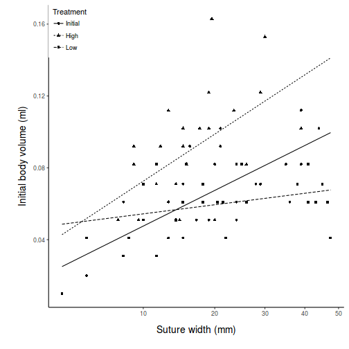
There is clear evidence that the relationships between suture width and initial volume differ between the three food regimes (slopes are not parallel and a significant interaction between food treatment and initial volume). Regular Ancova is not appropriate.
