Tutorial 9.4a - Split-plot and complex repeated measures ANOVA
27 Jul 2018
Overview
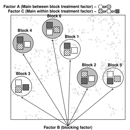
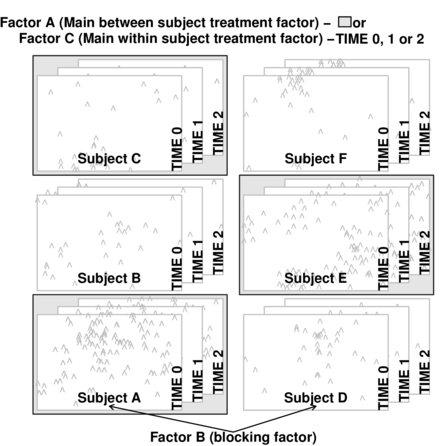
Split-plot designs (plots refer to agricultural field plots for which these designs were originally devised) extend unreplicated factorial (randomized complete block and simple repeated measures) designs by incorporating an additional factor whose levels are applied to entire blocks. Similarly, complex repeated measures designs are repeated measures designs in which there are different types of subjects. Split-plot and complex repeated measures designs are depicted diagrammatically in the following figure.
|
|
Consider the example of a randomized complete block presented at the start of Tutorial 9.3a. Blocks of four treatments (representing leaf packs subject to different aquatic taxa) were secured in numerous locations throughout a potentially heterogeneous stream. If some of those blocks had been placed in riffles, some in runs and some in pool habitats of the stream, the design becomes a split-plot design incorporating a between block factor (stream region: runs, riffles or pools) and a within block factor (leaf pack exposure type: microbial, macro invertebrate or vertebrate).
Furthermore, the design would enable us to investigate whether the roles that different organism scales play on the breakdown of leaf material in stream are consistent across each of the major regions of a stream (interaction between region and exposure type). Alternatively (or in addition), shading could be artificially applied to half of the blocks, thereby introducing a between block effect (whether the block is shaded or not).
Extending the repeated measures examples from Tutorial 9.3a, there might have been different populations (such as different species or histories) of rats or sharks. Any single subject (such as an individual shark or rat) can only be of one of the populations types and thus this additional factor represents a between subject effect.
Null hypotheses
There are separate null hypotheses associated with each of the main factors (and interactions), although typically, null hypotheses associated with the random blocking factors are of little interest.
Factor A - the main between block treatment effect
Fixed (typical case)
H$_0(A)$: $\mu_1=\mu_2=...=\mu_i=\mu$ (the population group means of A are all equal)
The mean of population 1 is equal to that of population 2 and so on, and thus all population means are equal to an overall mean. No effect of A.
If the effect of the $i^{th}$ group is the difference between the $i^{th}$ group mean and the overall mean ($\alpha_i = \mu_i - \mu$) then the H$_0$ can alternatively be written as:
H$_0(A)$: $\alpha_1 = \alpha_2 = ... = \alpha_i = 0$ \hspace*{2em}(the effect of each group equals zero)
If one or more of the $\alpha_i$ are different from zero (the response mean for this treatment differs from the overall response mean), the null hypothesis is not true indicating that the treatment does affect the response variable.
Random
H$_0(A)$: $\sigma_\alpha^2=0$ (population variance equals zero)
There is no added variance due to all possible levels of A.
Factor B - the blocking factor
Random (typical case)
H$_0(B)$: $\sigma_\beta^2=0$ (population variance equals zero)
There is no added variance due to all possible levels of B.
Fixed
H$_0(B)$: $\mu_{1}=\mu_{2}=...=\mu_{i}=\mu$ (the population group means of B are all equal)
H$_0(B)$: $\beta_{1} = \beta_{2}= ... = \beta_{i} = 0$ (the effect of each chosen B group equals zero)
Factor C - the main within block treatment effect
Fixed (typical case)
H$_0(C)$: $\mu_1=\mu_2=...=\mu_k=\mu$ (the population group means of C (pooling B) are all equal)
The mean of population 1 (pooling blocks) is equal to that of population 2 and so on, and thus all population means are equal to an overall mean. No effect of C within each block (Model 2) or over and above the effect of blocks.
If the effect of the $k^{th}$ group is the difference between the $k^{th}$ group mean and the overall mean ($\gamma_k = \mu_k - \mu$) then the H$_0$ can alternatively be written as:
H$_0(C)$: $\gamma_1 = \gamma_2 = ... = \gamma_k = 0$ (the effect of each group equals zero)
If one or more of the $\gamma_k$ are different from zero (the response mean for this treatment differs from the overall response mean), the null hypothesis is not true indicating that the treatment does affect the response variable.
Random
H$_0(C)$: $\sigma_\gamma^2=0$ (population variance equals zero)
There is no added variance due to all possible levels of C (pooling B).
Factor AC interaction - the main within block interaction effect
Fixed (typical case)
H$_0(A\times C)$: $\mu_{ijk}-\mu_i-\mu_k+\mu=0$ (the population group means of AC combinations (pooling B) are all equal)
There are no effects in addition to the main effects and the overall mean.
If the effect of the $ik^{th}$ group is the difference between the $ik^{th}$ group mean and the overall mean ($\gamma_{ik} = \mu_i - \mu$) then the H$_0$ can alternatively be written as:
H$_0(AC)$: $\alpha\gamma_{11} = \alpha\gamma_{12} = ... = \alpha\gamma_{ik} = 0$ (the interaction is equal to zero)
Random
H$_0(AC)$: $\sigma_{\alpha\gamma}^2=0$ (population variance equals zero)
There is no added variance due to any interaction effects (pooling B).
Factor BC interaction - the main within block by within Block effects
Random (typical case)
H$_0(BC)$: $\sigma_{\beta\gamma}^2=0$ (population variance equals zero)
There is no added variance due to any block by within block interaction effects. That is, the patterns amongst the levels of C are consistent across all the blocks.
Unless each of the levels of Factor C are replicated (occur more than once) within each block, this null hypotheses about this effect cannot be tested.
Linear models
The linear models for three and four factor partly nested designs are:
One between ($\alpha$), one within ($\gamma$) block effect
$y_{ijkl}=\mu+\alpha_i+\beta_{j}+\gamma_k+\alpha\gamma_{ij}+\beta\gamma_{jk} + \varepsilon_{ijkl}\hspace{20em}\\$
Two between ($\alpha$, $\gamma$), one within ($\delta$) block effect
\begin{align*} y_{ijklm}=&\mu+\alpha_i+\gamma_j+\alpha\gamma_{ij}+\beta_{k}+\delta_l+\alpha\delta_{il}+\gamma\delta_{jl} + \alpha\gamma\delta_{ijl}+\varepsilon_{ijklm}\hspace{5em} &\mathsf{(Model 2 - Additive)}\\ y_{ijklm}=&\mu+\alpha_i+\gamma_j+\alpha\gamma_{ij}+\beta_{k}+\delta_l+\alpha\delta_{il}+\gamma\delta_{jl} +\alpha\gamma\delta_{ijl} + \\ &\beta\delta_{kl}+\beta\alpha\delta_{kil}+\beta\gamma\delta_{kjl}+\beta\alpha\gamma\delta_{kijl}+\varepsilon_{ijklm}\hspace{5em} &\mathsf{(Model 1 - Non-additive)} \end{align*}One between ($\alpha$), two within ($\gamma$, $\delta$) block effects
\begin{align*} y_{ijklm}=&\mu+\alpha_i+\beta_{j}+\gamma_{k}+\delta_l+\gamma\delta_{kl}+\alpha\gamma_{ik}+\alpha\delta_{il}+\alpha\gamma\delta_{ikl}+\varepsilon_{ijk} \hspace{5em}&\mathsf{(Model 2- Additive)}\\ y_{ijklm}=&\mu+\alpha_i+\beta_{j}+\gamma_{k}+\beta\gamma_{jk}+\delta_l+\beta\delta_{jl}+\gamma\delta_{kl}+\beta\gamma\delta_{jkl}+\alpha\gamma_{ik}+\\ &\alpha\delta_{il}+\alpha\gamma\delta_{ikl}+\varepsilon_{ijk} &\mathsf{(Model 1 - Non-additive)} \end{align*} where $\mu$ is the overall mean, $\beta$ is the effect of the Blocking Factor B and $\varepsilon$ is the random unexplained or residual component.Analysis of Variance
The construction of appropriate F-ratios generally follow the rules and conventions established in Tutorial 8.7a-Tutorial 9.3a , albeit with additional complexity. The following tables document the (classically considered) appropriate numerator and denominator mean squares and degrees of freedom for each null hypothesis for a range of two and three factor partly nested designs. As stated in previous tutorials, there is considerable debate as to what the appropriate denominator degrees of freedom should be and indeed whether it is even possible to estimate the denominator degrees of freedom in hierarchical designs.
| F-ratio | |||||||||
|---|---|---|---|---|---|---|---|---|---|
| A&C fixed, B random | A fixed, B&C random | C fixed, A&B random | |||||||
| Factor | d.f | Restricted | Unrestricted | Restricted | Unrestricted | Restricted | Unrestricted | A,B&C random | |
| 1 | A | $a-1$ | 1/2 | 1/2 | 1/(2+4-5) | 1/(2+4-5) | 1/2 | ? | 1/(2+4-5) |
| 2 | B$^\prime$(A) | $(b-1)a$ | 2/5 | 2/5 | 2/5 | 2/5 | 2/5 | ||
| 3 | C | $(c-1)$ | 3/5 | 3/5 | 3/5 | 3/4 | 3/4 | 3/4 | 3/4 |
| 4 | AC | $(c-1)(a-1)$ | 4/5 | 4/5 | 4/5 | 4/5 | 4/5 | 4/5 | 4/5 |
| 5 | Resid (=CxB$^\prime$(A)) | $(c-1)(b-1)a$ | |||||||
| R syntax (A&C fixed, B random) | |||||||||
| Balanced |
summary(aov(y~A*C+Error(B), data)) |
||||||||
| Balanced or unbalanced |
library(nlme) summary(lme(y~A*C, random=~1|B, data)) summary(lme(y~A*C, random=~1|B, data), correlation=...) anova(lme(y~A*C, random=~1|B, data)) #OR library(lme4) summary(lmer(y~(1|B)+A*C, data)) |
||||||||
| Variance components |
library(nlme) summary(lme(y~1, random=~1|B/(A*C), data)) #OR library(lme4) summary(lmer(y~(1|B)+(1|A*C), data)) |
||||||||
Assumptions
As partly nested designs share elements in common with each of nested, factorial and unreplicated factorial designs, they also share similar assumptions and implications to these other designs. Readers should also consult the sections on assumptions in Tutorial 7.6a, Tutorial 9.2a and Tutorial 9.3a Specifically, hypothesis tests assume that:
- the appropriate residuals are normally distributed. Boxplots using the appropriate scale of replication (reflecting the appropriate residuals/F-ratio denominator (see Tables above) be used to explore normality. Scale transformations are often useful.
- the appropriate residuals are equally varied. Boxplots and plots of means against variance (using the appropriate scale of replication) should be used to explore the spread of values. Residual plots should reveal no patterns. Scale transformations are often useful.
- the appropriate residuals are independent of one another. Critically, experimental units within blocks/subjects should be adequately spaced temporally and spatially to restrict contamination or carryover effects. Non-independence resulting from the hierarchical design should be accounted for.
- that the variance/covariance matrix displays sphericity (strickly, the variance-covariance matrix must display a very specific pattern of sphericity in which both variances and covariances are equal (compound symmetry), however an F-ratio will still reliably follow an F distribution provided basic sphericity holds). This assumption is likely to be met only if the treatment levels within each block can be randomly ordered. This assumption can be managed by either adjusting the sensitivity of the affected F-ratios or employing linear mixed effects modelling to the design.
- there are no block by within block interactions. Such interactions render non-significant within block effects difficult to interpret unless we assume that there are no block by within block interactions, non-significant within block effects could be due to either an absence of a treatment effect, or as a result of opposing effects within different blocks. As these block by within block interactions are unreplicated, they can neither be formally tested nor is it possible to perform main effects tests to diagnose non-significant within block effects.
$R^2$ approximations
Whilst $R^2$ is a popular goodness of fit metric in simple linear models, its use is rarely extended to (generalized) linear mixed effects models. The reasons for this include:
- there are numerous ways that $R^2$ could be defined for mixed effects models, some of which can result in values that are either difficult to interpret or illogical (for example negative $R^2$).
- perhaps as a consequence, software implementation is also largely lacking.
Nakagawa and Schielzeth (2013) discuss the issues associated with $R^2$ calculations and
suggest a series of simple calculations to yield sensible $R^2$ values from mixed effects models.
An $R^2$ value quantifies the proportion of variance explained by a model (or by terms in a model) - the higher the
value, the better the model (or term) fit.
Nakagawa and Schielzeth (2013) offered up two $R^2$ for mixed effects models:
- Marginal $R^2$ - the proportion of total variance explained by the fixed effects. $$ \text{Marginal}~R^2 = \frac{\sigma^2_f}{\sigma^2_f + \sum^z_l{\sigma^2_l} + \sigma^2_d + \sigma^2_e} $$ where $\sigma^2_f$ is the variance of the fitted values (i.e. $\sigma^2_f = var(\mathbf{X\beta})$) on the link scale, $\sum^z_l{\sigma^2_l}$ is the sum of the $z$ random effects (including the residuals) and $\sigma^2_d$ and $\sigma^2_e$ are additional variance components appropriate when using non-Gaussian distributions.
- Conditional $R^2$ - the proportion of the total variance collectively explained by the fixed and random factors $$ \text{Conditional}~R^2 = \frac{\sigma^2_f + \sum^z_l{\sigma^2_l}}{\sigma^2_f + \sum^z_l{\sigma^2_l} + \sigma^2_d + \sigma^2_e} $$
Split-plot and complex repeated analysis in R
Split-plot design
Scenario and Data
Imagine we has designed an experiment in which we intend to measure a response ($y$) to one of treatments (three levels; 'a1', 'a2' and 'a3'). Unfortunately, the system that we intend to sample is spatially heterogeneous and thus will add a great deal of noise to the data that will make it difficult to detect a signal (impact of treatment).
Thus in an attempt to constrain this variability you decide to apply a design (RCB) in which each of the treatments within each of 35 blocks dispersed randomly throughout the landscape. As this section is mainly about the generation of artificial data (and not specifically about what to do with the data), understanding the actual details are optional and can be safely skipped. Consequently, I have folded (toggled) this section away.
- the number of between block treatments (A) = 3
- the number of blocks = 35
- the number of within block treatments (C) = 3
- the mean of the treatments = 40, 70 and 80 respectively
- the variability (standard deviation) between blocks of the same treatment = 12
- the variability (standard deviation) between treatments withing blocks = 5
library(ggplot2)
set.seed(1)
nA <- 3
nC <- 3
nBlock <- 36
sigma <- 5
sigma.block <- 12
n <- nBlock * nC
Block <- gl(nBlock, k = 1)
C <- gl(nC, k = 1)

## Specify the cell means
AC.means <- (rbind(c(40, 70, 80), c(35, 50, 70), c(35, 40, 45)))
## Convert these to effects
X <- model.matrix(~A * C, data = expand.grid(A = gl(3, k = 1), C = gl(3, k = 1)))
AC <- as.vector(AC.means)
AC.effects <- solve(X, AC)

A <- gl(nA, nBlock, n)
dt <- expand.grid(C = C, Block = Block)
dt <- data.frame(dt, A)

Xmat <- cbind(model.matrix(~-1 + Block, data = dt), model.matrix(~A * C, data = dt))
block.effects <- rnorm(n = nBlock, mean = 0, sd = sigma.block)
all.effects <- c(block.effects, AC.effects)
lin.pred <- Xmat %*% all.effects

## the quadrat observations (within sites) are drawn from normal distributions with means according to
## the site means and standard deviations of 5
y <- rnorm(n, lin.pred, sigma)
data.splt <- data.frame(y = y, A = A, dt)
head(data.splt)  #print out the first six rows of the data set
         y A C Block A.1
1 30.51110 1 1     1   1
2 62.18599 1 2     1   1
3 77.98268 1 3     1   1
4 46.01960 1 1     2   1
5 71.38110 1 2     2   1
6 80.93691 1 3     2   1
tapply(data.splt$y, data.splt$A, mean)
       1        2        3
67.73243 52.25684 37.79359
tapply(data.splt$y, data.splt$C, mean)
       1        2        3
37.57486 55.33468 64.87331
replications(y ~ A * C + Error(Block), data.splt)
  A   C A:C
 36  36  12
ggplot(data.splt, aes(y = y, x = C, linetype = A, group = A)) + geom_line(stat = "summary", fun.y = mean)

ggplot(data.splt, aes(y = y, x = C, color = A)) + geom_point() + facet_wrap(~Block)

Exploratory data analysis
Normality and Homogeneity of variance
# check between plot effects
library(plyr)
boxplot(y ~ A, ddply(data.splt, ~A + Block, summarise, y = mean(y)))

# OR
library(ggplot2)
ggplot(ddply(data.splt, ~A + Block, summarise, y = mean(y)), aes(y = y, x = A)) + geom_boxplot()

# check within plot effects
boxplot(y ~ A * C, data.splt)

# OR
ggplot(data.splt, aes(y = y, x = C, fill = A)) + geom_boxplot()

Conclusions:
- there is no evidence that the response variable is consistently non-normal across all populations - each boxplot is approximately symmetrical
- there is no evidence that variance (as estimated by the height of the boxplots) differs between the five populations. . More importantly, there is no evidence of a relationship between mean and variance - the height of boxplots does not increase with increasing position along the y-axis. Hence it there is no evidence of non-homogeneity
- transform the scale of the response variables (to address normality etc). Note transformations should be applied to the entire response variable (not just those populations that are skewed).
Block by within-Block interaction
library(car)
with(data.splt, interaction.plot(C, Block, y))

# OR with ggplot
library(ggplot2)
ggplot(data.splt, aes(y = y, x = C, group = Block, color = Block)) + geom_line() + guides(color = guide_legend(ncol = 3))

library(car)
residualPlots(lm(y ~ Block + A * C, data.splt))

           Test stat Pr(>|t|)
Block             NA       NA
A                 NA       NA
C                 NA       NA
Tukey test     1.539    0.124
# the Tukey's non-additivity test by itself can be obtained via an internal function within the car
# package
car:::tukeyNonaddTest(lm(y ~ Block + A * C, data.splt))
     Test    Pvalue
1.5394292 0.1236996
Conclusions:
- there is no visual or inferential evidence of any major interactions between Block and the within-Block effect (C). Any trends appear to be reasonably consistent between Blocks.
Sphericity
Prior to the use of maximum likelihood and mixed effects models (that permit specifying alternative variance-covariance structures), randomized block and repeated measures ANOVAs assumed that the variance-covariance matrix followed a specific pattern called 'Sphericity'. For repeated measures designs in which the within subject effects could not be randomized, the variance-covariance matrix was unlikely to meet sphericity. The only way of compensating for this was to estimate the degree to which sphericity was violated (via an epsilon value) and then use this epsilon to reduce the degrees of freedom of the model (thereby making p-values more conservative).
Since the levels of C in the current example were randomly assigned within each Block, we have no reason to expect that the variance-covariance will deviate substantially from sphericity. Nevertheless, we can calculate the epsilon sphericity values to confirm this. Recall that the closer the epsilon value is to 1, the greater the degree of sphericity compliance.
Note that sphericity only applies to within block effects..
library(biology)
Error in library(biology): there is no package called 'biology'
epsi.GG.HF(aov(y ~ Error(Block) + C, data = data.splt))
Error in eval(expr, envir, enclos): could not find function "epsi.GG.HF"
Conclusions:
- Both the Greenhouse-Geisser and Huynh-Feldt epsilons are reasonably close to one (they are both greater than 0.8), hence there is no evidence of correlation dependency structures.
Alternatively (and preferentially), we can explore whether there is an auto-correlation patterns in the residuals.
library(nlme)
data.splt.lme <- lme(y ~ A * C, random = ~1 | Block, data = data.splt)
acf(resid(data.splt.lme))

Conclusions:
- The autocorrelation factor (ACF) at a range of lags up to 20, indicate that there is not a strong pattern of a contagious structure running through the residuals. Note the ACF of lag 0 will always be 1 - the correlation of residuals with themselves must be 100%.
Model fitting or statistical analysis
There are numerous ways of fitting split-plot models in R.
Linear mixed effects modelling via the lme() function. This method is one of the original implementations in which separate variance-covariance matrices are incorporated into a interactive sequence of (generalized least squares) and maximum likelihood (actually REML) estimates of 'fixed' and 'random effects'.
Rather than fit just a single, simple random intercepts model, it is common to fit other related alternative models and explore which model fits the data best. For example, we could also fit a random intercepts and slope model. We could also explore other variance-covariance structures (autocorrelation or heterogeneity).
library(nlme)
# random intercept
data.splt.lme <- lme(y ~ A * C, random = ~1 | Block, data.splt, method = "REML")
# random intercept/slope
data.splt.lme1 <- lme(y ~ A * C, random = ~A | Block, data.splt, method = "REML")
anova(data.splt.lme, data.splt.lme1)
               Model df      AIC      BIC    logLik   Test   L.Ratio p-value
data.splt.lme      1 11 714.3519 742.8982 -346.1759
data.splt.lme1     2 16 723.5937 765.1156 -345.7968 1 vs 2 0.7582165  0.9796
More modern linear mixed effects modelling via the lmer() function. In contrast to the lme() function, the lmer() function supports are more complex combination of random effects (such as crossed random effects). However, unfortunately, it does not yet (and probably never will) have a mechanism to support specifying alternative covariance structures needed to accommodate spatial and temporal autocorrelation
library(lme4)
data.splt.lmer <- lmer(y ~ A * C + (1 | Block), data.splt, REML = TRUE)  #random intercept
data.splt.lmer1 <- lmer(y ~ A * C + (A | Block), data.splt, REML = TRUE,
    control = lmerControl(check.nobs.vs.nRE = "ignore"))  #random intercept/slope
anova(data.splt.lmer, data.splt.lmer1)
Data: data.splt
Models:
data.splt.lmer: y ~ A * C + (1 | Block)
data.splt.lmer1: y ~ A * C + (A | Block)
                Df    AIC    BIC  logLik deviance  Chisq Chi Df Pr(>Chisq)
data.splt.lmer  11 743.50 773.00 -360.75   721.50
data.splt.lmer1 16 752.67 795.59 -360.34   720.67 0.8271      5     0.9753
Mixed effects models can also be fit using the Template Model Builder automatic differentiation engine via the glmmTMB() function from a package with the same name. glmmTMB is able to fit similar models to lmer, yet can also incorporate more complex features such as zero inflation and temporal autocorrelation. Random effects are assumed to be Gaussian on the scale of the linear predictor and are integrated out via Laplace approximation. On the downsides, REML is not available for this technique yet and nor is Gauss-Hermite quadrature (which can be useful when dealing with small sample sizes and non-gaussian errors.
library(glmmTMB)
data.splt.glmmTMB <- glmmTMB(y ~ A * C + (1 | Block), data.splt)  #random intercept
data.splt.glmmTMB1 <- glmmTMB(y ~ A * C + (A | Block), data.splt)  #random intercept/slope
anova(data.splt.glmmTMB, data.splt.glmmTMB1)
Data: data.splt
Models:
data.splt.glmmTMB: y ~ A * C + (1 | Block), zi=~0, disp=~1
data.splt.glmmTMB1: y ~ A * C + (A | Block), zi=~0, disp=~1
                   Df   AIC BIC  logLik deviance Chisq Chi Df Pr(>Chisq)
data.splt.glmmTMB  11 743.5 773 -360.75    721.5
data.splt.glmmTMB1 16                                       5
Traditional OLS with multiple error strata using the aov() function. The aov() function is actually a wrapper for a specialized lm() call that defines multiple residual terms and thus adds some properties and class attributes to the fitted model that modify the output. This option is illustrated purely as a link to the past, it is no longer considered as robust or flexible as more modern techniques.
data.splt.aov <- aov(y ~ A * C + Error(Block), data.splt)
Model evaluation
Temporal autocorrelation
Before proceeding any further we should really explore whether we are likely to have an issue with temporal autocorrelation. The models assume that there are no temporal dependency issues. A good way to explore this is to examine the autocorrelation function. Essentially, this involves looking at the degree of correlation between residuals associated with times of incrementally greater temporal lags.
We have already observed that a model with random intercepts and random slopes fits better than a model with just random intercepts. It is possible that this is due to temporal autocorrelation. The random intercept/slope model might have fit the temporally autocorrelated data better, but if this is due to autocorrelation, then the random intercepts/slope model does not actually adress the underlying issue. Consequently, it is important to explore autocorrelation for both models and if there is any evidence of temporal autocorrelation, refit both models.
We can visualize the issue via linear mixed model formulation: $$ \begin{align} y_i &\sim{} N(\mu_i, \sigma^2)\\ \mu_i &= \mathbf{X}\boldsymbol{\beta} + \mathbf{Z}\mathbf{b}\\ \mathbf{b} &\sim{} MVN(0, \Sigma)\\ \end{align} $$ With a bit or rearranging, $\mathbf{b}$ and $\Sigma$ can represent a combination of random intercepts ($\mathbf{b}_0$) and autocorrelated residuals ($\Sigma_{AR}$): $$ \begin{align} b_{ij} &= \mathbf{b}_{0,ij} + \varepsilon_{ij}\\ \varepsilon_i &\sim{} \Sigma_{AR}\\ \end{align} $$ where $i$ are the blocks and $j$ are the observations.
The current simulated data has only three observations within each Block (one for each of the C treatments). Consequently, there temporal autocorrelation is not that meaningful. Nevertheless, for other data sets it could be an issue and should be investigated. Tutorial 9.3a provides a demonstration on how to explore temporal autocorrelation.
Residuals
As always, exploring the residuals can reveal issues of heteroscadacity, non-linearity and potential issues with autocorrelation. Note for lme() and lmer() residual plots use standardized (normalized) residuals rather than raw residuals as the former reflect changes to the variance-covariance matrix whereas the later do not.
The following function will be used for the production of some of the qqnormal plots.
qq.line = function(x) {
    # following four lines from base R's qqline()
    y <- quantile(x[!is.na(x)], c(0.25, 0.75))
    x <- qnorm(c(0.25, 0.75))
    slope <- diff(y)/diff(x)
    int <- y[1L] - slope * x[1L]
    return(c(int = int, slope = slope))
}
plot(data.splt.lme)

qqnorm(resid(data.splt.lme))
qqline(resid(data.splt.lme))

## plot residuals against each of the fixed effects
plot(resid(data.splt.lme) ~ data.splt.lme$data$A)

plot(resid(data.splt.lme) ~ data.splt.lme$data$C)

library(sjPlot)
plot_grid(plot_model(data.splt.lme, type = "diag"))

plot(data.splt.lmer)

plot(fitted(data.splt.lmer), residuals(data.splt.lmer, type = "pearson",
    scaled = TRUE))

ggplot(fortify(data.splt.lmer), aes(y = .scresid, x = .fitted)) +
    geom_point()

QQline = qq.line(fortify(data.splt.lmer)$.scresid)
ggplot(fortify(data.splt.lmer), aes(sample = .scresid)) + stat_qq() +
    geom_abline(intercept = QQline[1], slope = QQline[2])

qqnorm(resid(data.splt.lmer))
qqline(resid(data.splt.lmer))

## plot residuals against each of the fixed effects
ggplot(fortify(data.splt.lmer), aes(y = .scresid, x = A)) + geom_point()

ggplot(fortify(data.splt.lmer), aes(y = .scresid, x = C)) + geom_point()

library(sjPlot)
plot_grid(plot_model(data.splt.lmer, type = "diag"))

ggplot(data = NULL, aes(y = resid(data.splt.glmmTMB, type = "pearson"),
    x = fitted(data.splt.glmmTMB))) + geom_point()

QQline = qq.line(resid(data.splt.glmmTMB, type = "pearson"))
ggplot(data = NULL, aes(sample = resid(data.splt.glmmTMB, type = "pearson"))) +
    stat_qq() + geom_abline(intercept = QQline[1], slope = QQline[2])

ggplot(data = NULL, aes(y = resid(data.splt.glmmTMB, type = "pearson"),
    x = data.splt.glmmTMB$frame$A)) + geom_point()

ggplot(data = NULL, aes(y = resid(data.splt.glmmTMB, type = "pearson"),
    x = data.splt.glmmTMB$frame$C)) + geom_point()

library(sjPlot)
plot_grid(plot_model(data.splt.glmmTMB, type = "diag"))  #not working yet - bug
Error in UseMethod("rstudent"): no applicable method for 'rstudent' applied to an object of class "glmmTMB"
par(mfrow = c(2, 2))
plot(lm(data.splt.aov))

Exploring model parameters
If there was any evidence that the assumptions had been violated, then we would need to reconsider the model and start the process again. In this case, there is no evidence that the test will be unreliable so we can proceed to explore the test statistics. As I had elected to illustrate multiple techniques for analysing this nested design, I will also deal with the summaries etc separately.
Partial effects plots
It is often useful to visualize partial effects plots while exploring the parameter estimates. Having a graphical representation of the partial effects typically makes it a lot easier to interpret the parameter estimates and inferences.
library(effects)
plot(allEffects(data.splt.lme))

plot(allEffects(data.splt.lme), lines = list(multiline = TRUE),
    confint = list(style = "bars"))

library(sjPlot)
plot_model(data.splt.lme, type = "eff", terms = c("A", "C"))

library(effects)
plot(allEffects(data.splt.lmer))

plot(allEffects(data.splt.lmer), lines = list(multiline = TRUE),
    confint = list(style = "bars"))

library(sjPlot)
plot_model(data.splt.lmer, type = "eff", terms = c("A", "C"))

library(ggeffects)
# observation level effects averaged across margins
p = ggaverage(data.splt.glmmTMB, terms = c("A", "C"), x.as.factor = TRUE)
p = p %>% dplyr::rename(A = x, C = group)
ggplot(p, aes(y = predicted, x = A, color = C)) + geom_pointrange(aes(ymin = conf.low,
    ymax = conf.high))

# marginal effects
p = ggpredict(data.splt.glmmTMB, terms = c("A", "C"), x.as.factor = TRUE)
p = p %>% dplyr::rename(A = x, C = group)
ggplot(p, aes(y = predicted, x = A, color = C)) + geom_pointrange(aes(ymin = conf.low,
    ymax = conf.high))

Extractor functions
There are a number of extractor functions (functions that extract or derive specific information from a model) available including:| Extractor | Description |
|---|---|
| residuals() | Extracts the residuals from the model |
| fitted() | Extracts the predicted (expected) response values (on the link scale) at the observed levels of the linear predictor |
| predict() | Extracts the predicted (expected) response values (on either the link, response or terms (linear predictor) scale) |
| coef() | Extracts the model coefficients |
| confint() | Calculate confidence intervals for the model coefficients |
| summary() | Summarizes the important output and characteristics of the model |
| anova() | Computes an analysis of variance (variance partitioning) from the model |
| VarCorr() | Computes variance components (of random effects) from the model |
| AIC() | Computes Akaike Information Criterion from the model |
| plot() | Generates a series of diagnostic plots from the model |
| effect() | effects package - estimates the marginal (partial) effects of a factor (useful for plotting) |
| avPlot() | car package - generates partial regression plots |
Parameter estimates
summary(data.splt.lme)
Linear mixed-effects model fit by REML
 Data: data.splt
       AIC      BIC    logLik
  714.3519 742.8982 -346.1759

Random effects:
 Formula: ~1 | Block
        (Intercept) Residual
StdDev:    11.00689 4.309761

Fixed effects: y ~ A * C
                Value Std.Error DF    t-value p-value
(Intercept)  44.39871  3.412303 66  13.011362  0.0000
A2           -8.86091  4.825726 33  -1.836182  0.0754
A3          -11.61064  4.825726 33  -2.405988  0.0219
C2           31.17007  1.759453 66  17.715775  0.0000
C3           38.83108  1.759453 66  22.069979  0.0000
A2:C2       -15.33891  2.488242 66  -6.164556  0.0000
A3:C2       -24.89184  2.488242 66 -10.003787  0.0000
A2:C3        -4.50515  2.488242 66  -1.810574  0.0748
A3:C3       -30.09278  2.488242 66 -12.093993  0.0000
 Correlation:
      (Intr) A2     A3     C2     C3     A2:C2  A3:C2  A2:C3
A2    -0.707
A3    -0.707  0.500
C2    -0.258  0.182  0.182
C3    -0.258  0.182  0.182  0.500
A2:C2  0.182 -0.258 -0.129 -0.707 -0.354
A3:C2  0.182 -0.129 -0.258 -0.707 -0.354  0.500
A2:C3  0.182 -0.258 -0.129 -0.354 -0.707  0.500  0.250
A3:C3  0.182 -0.129 -0.258 -0.354 -0.707  0.250  0.500  0.500

Standardized Within-Group Residuals:
         Min           Q1          Med           Q3          Max
-1.908000844 -0.541899250  0.003782048  0.542865052  1.810720228

Number of Observations: 108
Number of Groups: 36
intervals(data.splt.lme)
Approximate 95% confidence intervals

 Fixed effects:
                 lower       est.       upper
(Intercept)  37.585829  44.398712  51.2115953
A2          -18.678921  -8.860908   0.9571044
A3          -21.428649 -11.610637  -1.7926243
C2           27.657207  31.170068  34.6829285
C3           35.318224  38.831084  42.3439451
A2:C2       -20.306842 -15.338907 -10.3709713
A3:C2       -29.859778 -24.891843 -19.9239073
A2:C3        -9.473081  -4.505146   0.4627894
A3:C3       -35.060715 -30.092780 -25.1248447
attr(,"label")
[1] "Fixed effects:"

 Random Effects:
  Level: Block
                   lower     est.    upper
sd((Intercept)) 8.540243 11.00689 14.18598

 Within-group standard error:
   lower     est.    upper
3.633843 4.309761 5.111405
anova(data.splt.lme)
            numDF denDF  F-value p-value
(Intercept)     1    66 781.9956  <.0001
A               2    33  21.1243  <.0001
C               2    66 372.0035  <.0001
A:C             4    66  52.5514  <.0001
library(broom)
tidy(data.splt.lme, effects = "fixed", conf.int = TRUE)
# A tibble: 9 x 5
  term        estimate std.error statistic  p.value
  <chr>          <dbl>     <dbl>     <dbl>    <dbl>
1 (Intercept)    44.4       3.41     13.0  6.94e-20
2 A2             -8.86      4.83     -1.84 7.54e- 2
3 A3            -11.6       4.83     -2.41 2.19e- 2
4 C2             31.2       1.76     17.7  8.88e-27
5 C3             38.8       1.76     22.1  3.55e-32
6 A2:C2         -15.3       2.49     -6.16 4.80e- 8
7 A3:C2         -24.9       2.49    -10.0  7.43e-15
8 A2:C3          -4.51      2.49     -1.81 7.48e- 2
9 A3:C3         -30.1       2.49    -12.1  2.12e-18
glance(data.splt.lme)
# A tibble: 1 x 5
  sigma logLik   AIC   BIC deviance
  <dbl>  <dbl> <dbl> <dbl> <lgl>
1  4.31  -346.  714.  743. NA
The output comprises:
- various information criterion (for model comparison)
- the random effects variance components
- the estimated standard deviation between Blocks is
11.006894 - the estimated standard deviation within treatments is
4.309761 - Blocks represent
71.8622571% of the variability (based on SD).
- the estimated standard deviation between Blocks is
- the fixed effects
- The effects parameter estimates along with their hypothesis tests
- There is evidence of an interaction between $A$ and $C$ - the nature of the trends between $A1$, $A2$ and $A3$ are not consistent between all levels of $C$ (and vice verse).
summary(data.splt.lmer)
Linear mixed model fit by REML ['lmerMod']
Formula: y ~ A * C + (1 | Block)
   Data: data.splt

REML criterion at convergence: 692.4

Scaled residuals:
     Min       1Q   Median       3Q      Max
-1.90800 -0.54190  0.00378  0.54287  1.81072

Random effects:
 Groups   Name        Variance Std.Dev.
 Block    (Intercept) 121.15   11.01
 Residual              18.57    4.31
Number of obs: 108, groups:  Block, 36

Fixed effects:
            Estimate Std. Error t value
(Intercept)   44.399      3.412  13.011
A2            -8.861      4.826  -1.836
A3           -11.611      4.826  -2.406
C2            31.170      1.759  17.716
C3            38.831      1.759  22.070
A2:C2        -15.339      2.488  -6.165
A3:C2        -24.892      2.488 -10.004
A2:C3         -4.505      2.488  -1.811
A3:C3        -30.093      2.488 -12.094

Correlation of Fixed Effects:
      (Intr) A2     A3     C2     C3     A2:C2  A3:C2  A2:C3
A2    -0.707
A3    -0.707  0.500
C2    -0.258  0.182  0.182
C3    -0.258  0.182  0.182  0.500
A2:C2  0.182 -0.258 -0.129 -0.707 -0.354
A3:C2  0.182 -0.129 -0.258 -0.707 -0.354  0.500
A2:C3  0.182 -0.258 -0.129 -0.354 -0.707  0.500  0.250
A3:C3  0.182 -0.129 -0.258 -0.354 -0.707  0.250  0.500  0.500
confint(data.splt.lmer)
                 2.5 %      97.5 %
.sig01        8.383249  13.6705563
.sigma        3.534158   4.9042634
(Intercept)  37.848710  50.9487139
A2          -18.124010   0.4021934
A3          -20.873738  -2.3475353
C2           27.823884  34.5162514
C3           35.484901  42.1772680
A2:C2       -20.071125 -10.6066884
A3:C2       -29.624061 -20.1596244
A2:C3        -9.237364   0.2270724
A3:C3       -34.824998 -25.3605618
anova(data.splt.lmer)
Analysis of Variance Table
    Df  Sum Sq Mean Sq F value
A    2   784.7   392.4  21.124
C    2 13819.2  6909.6 372.003
A:C  4  3904.4   976.1  52.551
library(broom)
tidy(data.splt.lmer, effects = "fixed", conf.int = TRUE)
# A tibble: 9 x 6
  term        estimate std.error statistic conf.low conf.high
  <chr>          <dbl>     <dbl>     <dbl>    <dbl>     <dbl>
1 (Intercept)    44.4       3.41     13.0     37.7     51.1
2 A2             -8.86      4.83     -1.84   -18.3      0.597
3 A3            -11.6       4.83     -2.41   -21.1     -2.15
4 C2             31.2       1.76     17.7     27.7     34.6
5 C3             38.8       1.76     22.1     35.4     42.3
6 A2:C2         -15.3       2.49     -6.16   -20.2    -10.5
7 A3:C2         -24.9       2.49    -10.0    -29.8    -20.0
8 A2:C3          -4.51      2.49     -1.81    -9.38     0.372
9 A3:C3         -30.1       2.49    -12.1    -35.0    -25.2
glance(data.splt.lmer)
# A tibble: 1 x 6
  sigma logLik   AIC   BIC deviance df.residual
  <dbl>  <dbl> <dbl> <dbl>    <dbl>       <int>
1  4.31  -346.  714.  744.     721.          97
As a result of disagreement and discontent concerning the appropriate residual degrees of freedom, lmer() does not provide p-values in summary or anova tables. For hypothesis testing, the following options exist:
- Confidence intervals on the estimated parameters.
confint(data.splt.lmer)
                 2.5 %      97.5 %
.sig01        8.383249  13.6705563
.sigma        3.534158   4.9042634
(Intercept)  37.848710  50.9487139
A2          -18.124010   0.4021934
A3          -20.873738  -2.3475353
C2           27.823884  34.5162514
C3           35.484901  42.1772680
A2:C2       -20.071125 -10.6066884
A3:C2       -29.624061 -20.1596244
A2:C3        -9.237364   0.2270724
A3:C3       -34.824998 -25.3605618
- Likelihood Ratio Test (LRT). Note, as this is contrasting a fixed component, the models need to be fitted with ML rather than REML.
mod1 = update(data.splt.lmer, REML = FALSE)
mod2 = update(data.splt.lmer, ~. - A, REML = FALSE)
anova(mod1, mod2)
Data: data.splt Models: mod1: y ~ A * C + (1 | Block) mod2: y ~ C + (1 | Block) + A:C Df AIC BIC logLik deviance Chisq Chi Df Pr(>Chisq) mod1 11 743.5 773 -360.75 721.5 mod2 11 743.5 773 -360.75 721.5 0 0 1 - Adopt the Satterthwaite or Kenward-Roger methods to denominator degrees of freedom (as used in SAS). This approach requires the lmerTest
and pbkrtest packages and requires that they be loaded before fitting the model (update() will suffice).
Note just because these are the approaches adopted by SAS, this does not mean that they are 'correct'.
library(lmerTest)
data.splt.lmer <- update(data.splt.lmer)
summary(data.splt.lmer)
Linear mixed model fit by REML t-tests use Satterthwaite approximations to degrees of freedom [ lmerMod] Formula: y ~ A * C + (1 | Block) Data: data.splt REML criterion at convergence: 692.4 Scaled residuals: Min 1Q Median 3Q Max -1.90800 -0.54190 0.00378 0.54287 1.81072 Random effects: Groups Name Variance Std.Dev. Block (Intercept) 121.15 11.01 Residual 18.57 4.31 Number of obs: 108, groups: Block, 36 Fixed effects: Estimate Std. Error df t value Pr(>|t|) (Intercept) 44.399 3.412 39.543 13.011 6.66e-16 *** A2 -8.861 4.826 39.543 -1.836 0.0739 . A3 -11.611 4.826 39.543 -2.406 0.0209 * C2 31.170 1.759 66.000 17.716 < 2e-16 *** C3 38.831 1.759 66.000 22.070 < 2e-16 *** A2:C2 -15.339 2.488 66.000 -6.165 4.80e-08 *** A3:C2 -24.892 2.488 66.000 -10.004 7.55e-15 *** A2:C3 -4.505 2.488 66.000 -1.811 0.0748 . A3:C3 -30.093 2.488 66.000 -12.094 < 2e-16 *** --- Signif. codes: 0 '***' 0.001 '**' 0.01 '*' 0.05 '.' 0.1 ' ' 1 Correlation of Fixed Effects: (Intr) A2 A3 C2 C3 A2:C2 A3:C2 A2:C3 A2 -0.707 A3 -0.707 0.500 C2 -0.258 0.182 0.182 C3 -0.258 0.182 0.182 0.500 A2:C2 0.182 -0.258 -0.129 -0.707 -0.354 A3:C2 0.182 -0.129 -0.258 -0.707 -0.354 0.500 A2:C3 0.182 -0.258 -0.129 -0.354 -0.707 0.500 0.250 A3:C3 0.182 -0.129 -0.258 -0.354 -0.707 0.250 0.500 0.500anova(data.splt.lmer) # Satterthwaite denominator df method
Analysis of Variance Table of type III with Satterthwaite approximation for degrees of freedom Sum Sq Mean Sq NumDF DenDF F.value Pr(>F) A 784.7 392.4 2 33 21.12 1.24e-06 *** C 13819.2 6909.6 2 66 372.00 < 2.2e-16 *** A:C 3904.4 976.1 4 66 52.55 < 2.2e-16 *** --- Signif. codes: 0 '***' 0.001 '**' 0.01 '*' 0.05 '.' 0.1 ' ' 1anova(data.splt.lmer, ddf = "Kenward-Roger")
Analysis of Variance Table of type III  with  Kenward-Roger
approximation for degrees of freedom
     Sum Sq Mean Sq NumDF DenDF F.value    Pr(>F)
A     784.7   392.4     2    33   21.12  1.24e-06 ***
C   13819.2  6909.6     2    66  372.00 < 2.2e-16 ***
A:C  3904.4   976.1     4    66   52.55 < 2.2e-16 ***
---
Signif. codes:  0 '***' 0.001 '**' 0.01 '*' 0.05 '.' 0.1 ' ' 1
The output comprises:
- various information criterion (for model comparison)
- the random effects variance components
- the estimated standard deviation between Blocks is
11.0068942 - the estimated standard deviation within treatments is
4.3097613 - Blocks represent
71.8622559% of the variability (based on SD).
- the estimated standard deviation between Blocks is
- the fixed effects
- The effects parameter estimates along with their hypothesis tests
- There is evidence of an interaction between $A$ and $C$ - the nature of the trends between $A1$, $A2$ and $A3$ are not consistent between all levels of $C$ (and vice verse).
summary(data.splt.glmmTMB)
 Family: gaussian  ( identity )
Formula:          y ~ A * C + (1 | Block)
Data: data.splt

     AIC      BIC   logLik deviance df.resid
   743.5    773.0   -360.7    721.5       97

Random effects:

Conditional model:
 Groups   Name        Variance Std.Dev.
 Block    (Intercept) 111.06   10.538
 Residual              17.03    4.126
Number of obs: 108, groups:  Block, 36

Dispersion estimate for gaussian family (sigma^2):   17

Conditional model:
            Estimate Std. Error z value Pr(>|z|)
(Intercept)   44.399      3.267  13.590  < 2e-16 ***
A2            -8.861      4.620  -1.918   0.0551 .
A3           -11.611      4.620  -2.513   0.0120 *
C2            31.170      1.685  18.504  < 2e-16 ***
C3            38.831      1.685  23.051  < 2e-16 ***
A2:C2        -15.339      2.382  -6.439 1.21e-10 ***
A3:C2        -24.892      2.382 -10.449  < 2e-16 ***
A2:C3         -4.505      2.382  -1.891   0.0586 .
A3:C3        -30.093      2.382 -12.632  < 2e-16 ***
---
Signif. codes:  0 '***' 0.001 '**' 0.01 '*' 0.05 '.' 0.1 ' ' 1
confint(data.splt.glmmTMB)
                                    2.5 %      97.5 %   Estimate
cond.(Intercept)                37.995459  50.8019809  44.398720
cond.A2                        -17.916505   0.1946518  -8.860926
cond.A3                        -20.666227  -2.5550708 -11.610649
cond.C2                         27.868417  34.4717213  31.170069
cond.C3                         35.529441  42.1327460  38.831094
cond.A2:C2                     -20.008147 -10.6696636 -15.338905
cond.A3:C2                     -29.561085 -20.2226021 -24.891844
cond.A2:C3                      -9.174404   0.1640792  -4.505162
cond.A3:C3                     -34.762032 -25.4235487 -30.092790
cond.Std.Dev.Block.(Intercept)   8.265449  13.4361251  10.538292
sigma                            3.504495   4.8583895   4.126282
The output comprises:
- various information criterion (for model comparison)
- the random effects variance components
- the estimated standard deviation between Blocks is
- the estimated standard deviation within treatments is
TRUE - Blocks represent % of the variability (based on SD).
- the fixed effects
- The effects parameter estimates along with their hypothesis tests
- There is evidence of an interaction between $A$ and $C$ - the nature of the trends between $A1$, $A2$ and $A3$ are not consistent between all levels of $C$ (and vice verse).
summary(data.splt.aov)
Error: Block
          Df Sum Sq Mean Sq F value   Pr(>F)
A          2  16140    8070   21.12 1.24e-06 ***
Residuals 33  12607     382
---
Signif. codes:  0 '***' 0.001 '**' 0.01 '*' 0.05 '.' 0.1 ' ' 1

Error: Within
          Df Sum Sq Mean Sq F value Pr(>F)
C          2  13819    6910  372.00 <2e-16 ***
A:C        4   3904     976   52.55 <2e-16 ***
Residuals 66   1226      19
---
Signif. codes:  0 '***' 0.001 '**' 0.01 '*' 0.05 '.' 0.1 ' ' 1
Planned comparisons and pairwise post-hoc tests
Similar to Tutorial 7.6a.html, we could apply manual adjustments to separate simple main effects tests or refit the model with modified interaction terms in order to explore the main effect of one factor at different levels of the other factor. Alternatively, we could just apply different contrasts to the existing fitted model.
As with non-heirarchical models, we can incorporate alternative contrasts for the fixed effects (other than the default treatment contrasts). The random factors must be sum-to-zero contrasts in order to ensure that the model is identifiable (possible to estimate true values of the parameters).
Likewise, post-hoc tests such as Tukey's tests can be performed.
For this demonstration, we have the extra complication - an interaction between A and C. For this reason, we will explore comparisons in A separately for each level of C (although we could do this the other way around and explore contrasts in C for each level of A).
In the absence of interactions, we could use glht() (which in this case, will perform the Tukey's test for A at the first level of C - as it is assumed in the absence of an interaction that this will be the same for all levels of C).
library(multcomp)
summary(glht(data.splt.lme, linfct = mcp(A = "Tukey")))
	 Simultaneous Tests for General Linear Hypotheses

Multiple Comparisons of Means: Tukey Contrasts


Fit: lme.formula(fixed = y ~ A * C, data = data.splt, random = ~1 |
    Block, method = "REML")

Linear Hypotheses:
           Estimate Std. Error z value Pr(>|z|)
2 - 1 == 0   -8.861      4.826  -1.836   0.1578
3 - 1 == 0  -11.611      4.826  -2.406   0.0427 *
3 - 2 == 0   -2.750      4.826  -0.570   0.8362
---
Signif. codes:  0 '***' 0.001 '**' 0.01 '*' 0.05 '.' 0.1 ' ' 1
(Adjusted p values reported -- single-step method)
confint(glht(data.splt.lme, linfct = mcp(A = "Tukey")))
	 Simultaneous Confidence Intervals

Multiple Comparisons of Means: Tukey Contrasts


Fit: lme.formula(fixed = y ~ A * C, data = data.splt, random = ~1 |
    Block, method = "REML")

Quantile = 2.3441
95% family-wise confidence level


Linear Hypotheses:
           Estimate lwr      upr
2 - 1 == 0  -8.8609 -20.1729   2.4511
3 - 1 == 0 -11.6106 -22.9227  -0.2986
3 - 2 == 0  -2.7497 -14.0617   8.5623
In this case, you will notice a message that warns us that we specified a model with an interaction term and that the above might not be appropriate. One alternative might be to perform the Tukey's test for A marginalizing (averaging) over all the levels of C.
As an alternative to the glht() function, we can also use the emmeans() function from a package with the same name. This package computes 'estimated marginal means' and is an adaptation of the least-squares (predicted marginal) means routine popularized by SAS. This routine uses the Kenward-Roger (or optionally, the Satterthwaite) method of calculating degrees of freedom and so will yield slightly different confidence intervals and p-values from glht(). Note, the emmeans() package has replaced the lsmeans() package.
library(multcomp)
summary(glht(data.splt.lme, linfct = mcp(A = "Tukey", interaction_average = TRUE)))
	 Simultaneous Tests for General Linear Hypotheses

Multiple Comparisons of Means: Tukey Contrasts


Fit: lme.formula(fixed = y ~ A * C, data = data.splt, random = ~1 |
    Block, method = "REML")

Linear Hypotheses:
           Estimate Std. Error z value Pr(>|z|)
2 - 1 == 0  -15.476      4.607  -3.359  0.00220 **
3 - 1 == 0  -29.939      4.607  -6.499  < 0.001 ***
3 - 2 == 0  -14.463      4.607  -3.139  0.00497 **
---
Signif. codes:  0 '***' 0.001 '**' 0.01 '*' 0.05 '.' 0.1 ' ' 1
(Adjusted p values reported -- single-step method)
confint(glht(data.splt.lme, linfct = mcp(A = "Tukey", interaction_average = TRUE)))
	 Simultaneous Confidence Intervals

Multiple Comparisons of Means: Tukey Contrasts


Fit: lme.formula(fixed = y ~ A * C, data = data.splt, random = ~1 |
    Block, method = "REML")

Quantile = 2.3431
95% family-wise confidence level


Linear Hypotheses:
           Estimate lwr      upr
2 - 1 == 0 -15.4756 -26.2702  -4.6810
3 - 1 == 0 -29.9388 -40.7334 -19.1443
3 - 2 == 0 -14.4633 -25.2578  -3.6687
## OR
library(emmeans)
emmeans(data.splt.lme, pairwise ~ A)
$emmeans
 A   emmean       SE df lower.CL upper.CL
 1 67.73243 3.257595 35 61.11916 74.34570
 2 52.25684 3.257595 33 45.62921 58.88446
 3 37.79359 3.257595 33 31.16596 44.42121

Results are averaged over the levels of: C
Degrees-of-freedom method: containment
Confidence level used: 0.95

$contrasts
 contrast estimate       SE df t.ratio p.value
 1 - 2    15.47559 4.606934 33   3.359  0.0055
 1 - 3    29.93884 4.606934 33   6.499  <.0001
 2 - 3    14.46325 4.606934 33   3.139  0.0097

Results are averaged over the levels of: C
P value adjustment: tukey method for comparing a family of 3 estimates
confint(emmeans(data.splt.lme, pairwise ~ A))
$emmeans
 A   emmean       SE df lower.CL upper.CL
 1 67.73243 3.257595 35 61.11916 74.34570
 2 52.25684 3.257595 33 45.62921 58.88446
 3 37.79359 3.257595 33 31.16596 44.42121

Results are averaged over the levels of: C
Degrees-of-freedom method: containment
Confidence level used: 0.95

$contrasts
 contrast estimate       SE df  lower.CL upper.CL
 1 - 2    15.47559 4.606934 33  4.171122 26.78006
 1 - 3    29.93884 4.606934 33 18.634374 41.24331
 2 - 3    14.46325 4.606934 33  3.158782 25.76772

Results are averaged over the levels of: C
Confidence level used: 0.95
Conf-level adjustment: tukey method for comparing a family of 3 estimates
Arguably, it would be better to perform the Tukey's test for A separately for each level of C.
library(emmeans)
emmeans(data.splt.lme, pairwise ~ A | C)
$emmeans
C = 1:
 A   emmean       SE df lower.CL upper.CL
 1 44.39871 3.412303 35 37.47137 51.32606
 2 35.53780 3.412303 33 28.59542 42.48019
 3 32.78808 3.412303 33 25.84569 39.73046

C = 2:
 A   emmean       SE df lower.CL upper.CL
 1 75.56878 3.412303 35 68.64144 82.49612
 2 51.36897 3.412303 33 44.42658 58.31135
 3 39.06630 3.412303 33 32.12392 46.00868

C = 3:
 A   emmean       SE df lower.CL upper.CL
 1 83.22980 3.412303 35 76.30245 90.15714
 2 69.86374 3.412303 33 62.92136 76.80613
 3 41.52638 3.412303 33 34.58400 48.46876

Degrees-of-freedom method: containment
Confidence level used: 0.95

$contrasts
C = 1:
 contrast  estimate       SE df t.ratio p.value
 1 - 2     8.860908 4.825726 33   1.836  0.1737
 1 - 3    11.610637 4.825726 33   2.406  0.0555
 2 - 3     2.749729 4.825726 33   0.570  0.8370

C = 2:
 contrast  estimate       SE df t.ratio p.value
 1 - 2    24.199815 4.825726 33   5.015  0.0001
 1 - 3    36.502479 4.825726 33   7.564  <.0001
 2 - 3    12.302665 4.825726 33   2.549  0.0404

C = 3:
 contrast  estimate       SE df t.ratio p.value
 1 - 2    13.366054 4.825726 33   2.770  0.0242
 1 - 3    41.703417 4.825726 33   8.642  <.0001
 2 - 3    28.337363 4.825726 33   5.872  <.0001

P value adjustment: tukey method for comparing a family of 3 estimates
confint(emmeans(data.splt.lme, pairwise ~ A | C))
$emmeans
C = 1:
 A   emmean       SE df lower.CL upper.CL
 1 44.39871 3.412303 35 37.47137 51.32606
 2 35.53780 3.412303 33 28.59542 42.48019
 3 32.78808 3.412303 33 25.84569 39.73046

C = 2:
 A   emmean       SE df lower.CL upper.CL
 1 75.56878 3.412303 35 68.64144 82.49612
 2 51.36897 3.412303 33 44.42658 58.31135
 3 39.06630 3.412303 33 32.12392 46.00868

C = 3:
 A   emmean       SE df lower.CL upper.CL
 1 83.22980 3.412303 35 76.30245 90.15714
 2 69.86374 3.412303 33 62.92136 76.80613
 3 41.52638 3.412303 33 34.58400 48.46876

Degrees-of-freedom method: containment
Confidence level used: 0.95

$contrasts
C = 1:
 contrast  estimate       SE df   lower.CL upper.CL
 1 - 2     8.860908 4.825726 33 -2.9804308 20.70225
 1 - 3    11.610637 4.825726 33 -0.2307022 23.45198
 2 - 3     2.749729 4.825726 33 -9.0916102 14.59107

C = 2:
 contrast  estimate       SE df   lower.CL upper.CL
 1 - 2    24.199815 4.825726 33 12.3584757 36.04115
 1 - 3    36.502479 4.825726 33 24.6611403 48.34382
 2 - 3    12.302665 4.825726 33  0.4613257 24.14400

C = 3:
 contrast  estimate       SE df   lower.CL upper.CL
 1 - 2    13.366054 4.825726 33  1.5247149 25.20739
 1 - 3    41.703417 4.825726 33 29.8620777 53.54476
 2 - 3    28.337363 4.825726 33 16.4960239 40.17870

Confidence level used: 0.95
Conf-level adjustment: tukey method for comparing a family of 3 estimates
## For those who like their ANOVA
test(emmeans(data.splt.lme, specs = ~A | C), joint = TRUE)
 C df1 df2 F.ratio p.value
 1   3  35 123.363  <.0001
 2   3  NA 282.713  <.0001
 3   3  NA 387.404  <.0001
## OR
library(multcomp)
summary(glht(data.splt.lme, linfct = lsm(tukey ~ A | C)))
$`C = 1`

	 Simultaneous Tests for General Linear Hypotheses

Fit: lme.formula(fixed = y ~ A * C, data = data.splt, random = ~1 |
    Block, method = "REML")

Linear Hypotheses:
           Estimate Std. Error t value Pr(>|t|)
1 - 2 == 0    8.861      4.826   1.836   0.1737
1 - 3 == 0   11.611      4.826   2.406   0.0556 .
2 - 3 == 0    2.750      4.826   0.570   0.8370
---
Signif. codes:  0 '***' 0.001 '**' 0.01 '*' 0.05 '.' 0.1 ' ' 1
(Adjusted p values reported -- single-step method)


$`C = 2`

	 Simultaneous Tests for General Linear Hypotheses

Fit: lme.formula(fixed = y ~ A * C, data = data.splt, random = ~1 |
    Block, method = "REML")

Linear Hypotheses:
           Estimate Std. Error t value Pr(>|t|)
1 - 2 == 0   24.200      4.826   5.015   <0.001 ***
1 - 3 == 0   36.502      4.826   7.564   <0.001 ***
2 - 3 == 0   12.303      4.826   2.549   0.0403 *
---
Signif. codes:  0 '***' 0.001 '**' 0.01 '*' 0.05 '.' 0.1 ' ' 1
(Adjusted p values reported -- single-step method)


$`C = 3`

	 Simultaneous Tests for General Linear Hypotheses

Fit: lme.formula(fixed = y ~ A * C, data = data.splt, random = ~1 |
    Block, method = "REML")

Linear Hypotheses:
           Estimate Std. Error t value Pr(>|t|)
1 - 2 == 0   13.366      4.826   2.770   0.0242 *
1 - 3 == 0   41.703      4.826   8.642   <0.001 ***
2 - 3 == 0   28.337      4.826   5.872   <0.001 ***
---
Signif. codes:  0 '***' 0.001 '**' 0.01 '*' 0.05 '.' 0.1 ' ' 1
(Adjusted p values reported -- single-step method)
## OR
summary(glht(data.splt.lme, linfct = lsm(pairwise ~ A | C)))
$`C = 1`

	 Simultaneous Tests for General Linear Hypotheses

Fit: lme.formula(fixed = y ~ A * C, data = data.splt, random = ~1 |
    Block, method = "REML")

Linear Hypotheses:
           Estimate Std. Error t value Pr(>|t|)
1 - 2 == 0    8.861      4.826   1.836   0.1737
1 - 3 == 0   11.611      4.826   2.406   0.0556 .
2 - 3 == 0    2.750      4.826   0.570   0.8370
---
Signif. codes:  0 '***' 0.001 '**' 0.01 '*' 0.05 '.' 0.1 ' ' 1
(Adjusted p values reported -- single-step method)


$`C = 2`

	 Simultaneous Tests for General Linear Hypotheses

Fit: lme.formula(fixed = y ~ A * C, data = data.splt, random = ~1 |
    Block, method = "REML")

Linear Hypotheses:
           Estimate Std. Error t value Pr(>|t|)
1 - 2 == 0   24.200      4.826   5.015   <0.001 ***
1 - 3 == 0   36.502      4.826   7.564   <0.001 ***
2 - 3 == 0   12.303      4.826   2.549   0.0404 *
---
Signif. codes:  0 '***' 0.001 '**' 0.01 '*' 0.05 '.' 0.1 ' ' 1
(Adjusted p values reported -- single-step method)


$`C = 3`

	 Simultaneous Tests for General Linear Hypotheses

Fit: lme.formula(fixed = y ~ A * C, data = data.splt, random = ~1 |
    Block, method = "REML")

Linear Hypotheses:
           Estimate Std. Error t value Pr(>|t|)
1 - 2 == 0   13.366      4.826   2.770   0.0241 *
1 - 3 == 0   41.703      4.826   8.642   <0.001 ***
2 - 3 == 0   28.337      4.826   5.872   <0.001 ***
---
Signif. codes:  0 '***' 0.001 '**' 0.01 '*' 0.05 '.' 0.1 ' ' 1
(Adjusted p values reported -- single-step method)
confint(glht(data.splt.lme, linfct = lsm(tukey ~ A | C)))
$`C = 1`

	 Simultaneous Confidence Intervals

Fit: lme.formula(fixed = y ~ A * C, data = data.splt, random = ~1 |
    Block, method = "REML")

Quantile = 2.4539
95% family-wise confidence level


Linear Hypotheses:
           Estimate lwr     upr
1 - 2 == 0  8.8609  -2.9809 20.7028
1 - 3 == 0 11.6106  -0.2312 23.4525
2 - 3 == 0  2.7497  -9.0921 14.5916


$`C = 2`

	 Simultaneous Confidence Intervals

Fit: lme.formula(fixed = y ~ A * C, data = data.splt, random = ~1 |
    Block, method = "REML")

Quantile = 2.4539
95% family-wise confidence level


Linear Hypotheses:
           Estimate lwr     upr
1 - 2 == 0 24.1998  12.3580 36.0416
1 - 3 == 0 36.5025  24.6607 48.3442
2 - 3 == 0 12.3027   0.4609 24.1444


$`C = 3`

	 Simultaneous Confidence Intervals

Fit: lme.formula(fixed = y ~ A * C, data = data.splt, random = ~1 |
    Block, method = "REML")

Quantile = 2.4532
95% family-wise confidence level


Linear Hypotheses:
           Estimate lwr     upr
1 - 2 == 0 13.3661   1.5278 25.2043
1 - 3 == 0 41.7034  29.8651 53.5417
2 - 3 == 0 28.3374  16.4991 40.1757
Comp1: Group 2 vs Group 3
Comp2: Group 1 vs (Group 2,3)
## Planned contrasts 1.(A2 vs A3) 2.(A1 vs A2,A3)
contr.A = cbind(c(0, 1, -1), c(1, -0.5, -0.5))
crossprod(contr.A)
     [,1] [,2]
[1,]    2  0.0
[2,]    0  1.5
emmeans(data.splt.lme, spec = "A", by = "C", contr = list(A = contr.A))
$emmeans
C = 1:
 A   emmean       SE df lower.CL upper.CL
 1 44.39871 3.412303 35 37.47137 51.32606
 2 35.53780 3.412303 33 28.59542 42.48019
 3 32.78808 3.412303 33 25.84569 39.73046

C = 2:
 A   emmean       SE df lower.CL upper.CL
 1 75.56878 3.412303 35 68.64144 82.49612
 2 51.36897 3.412303 33 44.42658 58.31135
 3 39.06630 3.412303 33 32.12392 46.00868

C = 3:
 A   emmean       SE df lower.CL upper.CL
 1 83.22980 3.412303 35 76.30245 90.15714
 2 69.86374 3.412303 33 62.92136 76.80613
 3 41.52638 3.412303 33 34.58400 48.46876

Degrees-of-freedom method: containment
Confidence level used: 0.95

$contrasts
C = 1:
 contrast  estimate       SE df t.ratio p.value
 A.1       2.749729 4.825726 33   0.570  0.5727
 A.2      10.235772 4.179201 33   2.449  0.0198

C = 2:
 contrast  estimate       SE df t.ratio p.value
 A.1      12.302665 4.825726 33   2.549  0.0156
 A.2      30.351147 4.179201 33   7.262  <.0001

C = 3:
 contrast  estimate       SE df t.ratio p.value
 A.1      28.337363 4.825726 33   5.872  <.0001
 A.2      27.534735 4.179201 33   6.589  <.0001
contrast(emmeans(data.splt.lme, ~A | C), method = list(A = contr.A))
C = 1:
 contrast  estimate       SE df t.ratio p.value
 A.1       2.749729 4.825726 33   0.570  0.5727
 A.2      10.235772 4.179201 33   2.449  0.0198

C = 2:
 contrast  estimate       SE df t.ratio p.value
 A.1      12.302665 4.825726 33   2.549  0.0156
 A.2      30.351147 4.179201 33   7.262  <.0001

C = 3:
 contrast  estimate       SE df t.ratio p.value
 A.1      28.337363 4.825726 33   5.872  <.0001
 A.2      27.534735 4.179201 33   6.589  <.0001
confint(contrast(emmeans(data.splt.lme, ~A | C), method = list(A = contr.A)))
C = 1:
 contrast  estimate       SE df  lower.CL upper.CL
 A.1       2.749729 4.825726 33 -7.068284 12.56774
 A.2      10.235772 4.179201 33  1.733124 18.73842

C = 2:
 contrast  estimate       SE df  lower.CL upper.CL
 A.1      12.302665 4.825726 33  2.484652 22.12068
 A.2      30.351147 4.179201 33 21.848499 38.85380

C = 3:
 contrast  estimate       SE df  lower.CL upper.CL
 A.1      28.337363 4.825726 33 18.519350 38.15538
 A.2      27.534735 4.179201 33 19.032087 36.03738

Confidence level used: 0.95
## Using glht
summary(glht(data.splt.lme, linfct = lsm("A", by = "C", contr = list(A = contr.A))),
    test = adjusted("none"))
$`C = 1`

	 Simultaneous Tests for General Linear Hypotheses

Fit: lme.formula(fixed = y ~ A * C, data = data.splt, random = ~1 |
    Block, method = "REML")

Linear Hypotheses:
         Estimate Std. Error t value Pr(>|t|)
A.1 == 0    2.750      4.826   0.570   0.5727
A.2 == 0   10.236      4.179   2.449   0.0198 *
---
Signif. codes:  0 '***' 0.001 '**' 0.01 '*' 0.05 '.' 0.1 ' ' 1
(Adjusted p values reported -- none method)


$`C = 2`

	 Simultaneous Tests for General Linear Hypotheses

Fit: lme.formula(fixed = y ~ A * C, data = data.splt, random = ~1 |
    Block, method = "REML")

Linear Hypotheses:
         Estimate Std. Error t value Pr(>|t|)
A.1 == 0   12.303      4.826   2.549   0.0156 *
A.2 == 0   30.351      4.179   7.262 2.48e-08 ***
---
Signif. codes:  0 '***' 0.001 '**' 0.01 '*' 0.05 '.' 0.1 ' ' 1
(Adjusted p values reported -- none method)


$`C = 3`

	 Simultaneous Tests for General Linear Hypotheses

Fit: lme.formula(fixed = y ~ A * C, data = data.splt, random = ~1 |
    Block, method = "REML")

Linear Hypotheses:
         Estimate Std. Error t value Pr(>|t|)
A.1 == 0   28.337      4.826   5.872 1.41e-06 ***
A.2 == 0   27.535      4.179   6.589 1.73e-07 ***
---
Signif. codes:  0 '***' 0.001 '**' 0.01 '*' 0.05 '.' 0.1 ' ' 1
(Adjusted p values reported -- none method)
confint(glht(data.splt.lme, linfct = lsm("A", by = "C", contr = list(A = contr.A))),
    calpha = univariate_calpha())
$`C = 1`

	 Simultaneous Confidence Intervals

Fit: lme.formula(fixed = y ~ A * C, data = data.splt, random = ~1 |
    Block, method = "REML")

Quantile = 2.0345
95% confidence level


Linear Hypotheses:
         Estimate lwr     upr
A.1 == 0  2.7497  -7.0683 12.5677
A.2 == 0 10.2358   1.7331 18.7384


$`C = 2`

	 Simultaneous Confidence Intervals

Fit: lme.formula(fixed = y ~ A * C, data = data.splt, random = ~1 |
    Block, method = "REML")

Quantile = 2.0345
95% confidence level


Linear Hypotheses:
         Estimate lwr     upr
A.1 == 0 12.3027   2.4847 22.1207
A.2 == 0 30.3511  21.8485 38.8538


$`C = 3`

	 Simultaneous Confidence Intervals

Fit: lme.formula(fixed = y ~ A * C, data = data.splt, random = ~1 |
    Block, method = "REML")

Quantile = 2.0345
95% confidence level


Linear Hypotheses:
         Estimate lwr     upr
A.1 == 0 28.3374  18.5194 38.1554
A.2 == 0 27.5347  19.0321 36.0374
## OR manually
newdata = with(data.splt, expand.grid(A = levels(A), C = levels(C)))
Xmat = model.matrix(~A * C, newdata)
coefs = fixef(data.splt.lme)
Xmat.split = split.data.frame(Xmat, f = newdata$C)
## When estimating the confidence intervals, we will base Q on model
## degrees of freedom lsmean uses Q=1.96
lapply(Xmat.split, function(x) {
    Xmat = t(t(x) %*% contr.A)
    fit = as.vector(coefs %*% t(Xmat))
    se = sqrt(diag(Xmat %*% vcov(data.splt.lme) %*% t(Xmat)))
    Q = qt(0.975, data.splt.lme$fixDF$terms["A"])
    # Q=1.96
    data.frame(fit = fit, lower = fit - Q * se, upper = fit + Q * se)
})
$`1`
        fit     lower    upper
1  2.749729 -7.068284 12.56774
2 10.235772  1.733124 18.73842

$`2`
       fit     lower    upper
1 12.30266  2.484652 22.12068
2 30.35115 21.848499 38.85380

$`3`
       fit    lower    upper
1 28.33736 18.51935 38.15538
2 27.53474 19.03209 36.03738
## We could alternatively use the split contrast matrices directly in
## glht unfortunately, we then need to know what each row refers to...
contr.split = lapply(Xmat.split, function(x) {
    t(t(x) %*% contr.A)
})
contr.split = do.call("rbind", contr.split)
summary(glht(data.splt.lme, linfct = contr.split), test = adjusted("none"))
	 Simultaneous Tests for General Linear Hypotheses

Fit: lme.formula(fixed = y ~ A * C, data = data.splt, random = ~1 |
    Block, method = "REML")

Linear Hypotheses:
       Estimate Std. Error z value Pr(>|z|)
1 == 0    2.750      4.826   0.570   0.5688
2 == 0   10.236      4.179   2.449   0.0143 *
3 == 0   12.303      4.826   2.549   0.0108 *
4 == 0   30.351      4.179   7.262 3.80e-13 ***
5 == 0   28.337      4.826   5.872 4.30e-09 ***
6 == 0   27.535      4.179   6.589 4.44e-11 ***
---
Signif. codes:  0 '***' 0.001 '**' 0.01 '*' 0.05 '.' 0.1 ' ' 1
(Adjusted p values reported -- none method)
confint(glht(data.splt.lme, linfct = contr.split), calpha = univariate_calpha())
	 Simultaneous Confidence Intervals

Fit: lme.formula(fixed = y ~ A * C, data = data.splt, random = ~1 |
    Block, method = "REML")

Quantile = 1.96
95% confidence level


Linear Hypotheses:
       Estimate lwr     upr
1 == 0  2.7497  -6.7085 12.2080
2 == 0 10.2358   2.0447 18.4269
3 == 0 12.3027   2.8444 21.7609
4 == 0 30.3511  22.1601 38.5422
5 == 0 28.3374  18.8791 37.7956
6 == 0 27.5347  19.3437 35.7258
In the absence of interactions, we could use glht() (which in this case, will perform the Tukey's test for A at the first level of C - as it is assumed in the absence of an interaction that this will be the same for all levels of C).
library(multcomp)
summary(glht(data.splt.lmer, linfct = mcp(A = "Tukey")))
	 Simultaneous Tests for General Linear Hypotheses

Multiple Comparisons of Means: Tukey Contrasts


Fit: lme4::lmer(formula = y ~ A * C + (1 | Block), data = data.splt,
    REML = TRUE)

Linear Hypotheses:
           Estimate Std. Error z value Pr(>|z|)
2 - 1 == 0   -8.861      4.826  -1.836   0.1579
3 - 1 == 0  -11.611      4.826  -2.406   0.0427 *
3 - 2 == 0   -2.750      4.826  -0.570   0.8362
---
Signif. codes:  0 '***' 0.001 '**' 0.01 '*' 0.05 '.' 0.1 ' ' 1
(Adjusted p values reported -- single-step method)
confint(glht(data.splt.lmer, linfct = mcp(A = "Tukey")))
	 Simultaneous Confidence Intervals

Multiple Comparisons of Means: Tukey Contrasts


Fit: lme4::lmer(formula = y ~ A * C + (1 | Block), data = data.splt,
    REML = TRUE)

Quantile = 2.3442
95% family-wise confidence level


Linear Hypotheses:
           Estimate lwr      upr
2 - 1 == 0  -8.8609 -20.1734   2.4516
3 - 1 == 0 -11.6106 -22.9231  -0.2982
3 - 2 == 0  -2.7497 -14.0622   8.5627
In this case, you will notice a message that warns us that we specified a model with an interaction term and that the above might not be appropriate. One alternative might be to perform the Tukey's test for A marginalizing (averaging) over all the levels of C.
As an alternative to the glht() function, we can also use the emmeans() function from a package with the same name. This package computes 'estimated marginal means' and is an adaptation of the least-squares (predicted marginal) means routine popularized by SAS. This routine uses the Kenward-Roger (or optionally, the Satterthwaite) method of calculating degrees of freedom and so will yield slightly different confidence intervals and p-values from glht(). Note, the emmeans() package has replaced the lsmeans() package.
library(multcomp)
summary(glht(data.splt.lmer, linfct = mcp(A = "Tukey", interaction_average = TRUE)))
	 Simultaneous Tests for General Linear Hypotheses

Multiple Comparisons of Means: Tukey Contrasts


Fit: lme4::lmer(formula = y ~ A * C + (1 | Block), data = data.splt,
    REML = TRUE)

Linear Hypotheses:
           Estimate Std. Error z value Pr(>|z|)
2 - 1 == 0  -15.476      4.607  -3.359  0.00238 **
3 - 1 == 0  -29.939      4.607  -6.499  < 0.001 ***
3 - 2 == 0  -14.463      4.607  -3.139  0.00468 **
---
Signif. codes:  0 '***' 0.001 '**' 0.01 '*' 0.05 '.' 0.1 ' ' 1
(Adjusted p values reported -- single-step method)
confint(glht(data.splt.lmer, linfct = mcp(A = "Tukey", interaction_average = TRUE)))
	 Simultaneous Confidence Intervals

Multiple Comparisons of Means: Tukey Contrasts


Fit: lme4::lmer(formula = y ~ A * C + (1 | Block), data = data.splt,
    REML = TRUE)

Quantile = 2.3434
95% family-wise confidence level


Linear Hypotheses:
           Estimate lwr      upr
2 - 1 == 0 -15.4756 -26.2713  -4.6798
3 - 1 == 0 -29.9388 -40.7346 -19.1431
3 - 2 == 0 -14.4633 -25.2590  -3.6675
## OR
library(emmeans)
emmeans(data.splt.lmer, pairwise ~ A)
$emmeans
 A   emmean       SE df lower.CL upper.CL
 1 67.73243 3.257595 33 61.10480 74.36006
 2 52.25684 3.257595 33 45.62921 58.88446
 3 37.79359 3.257595 33 31.16596 44.42121

Results are averaged over the levels of: C
Degrees-of-freedom method: kenward-roger
Confidence level used: 0.95

$contrasts
 contrast estimate       SE df t.ratio p.value
 1 - 2    15.47559 4.606934 33   3.359  0.0055
 1 - 3    29.93884 4.606934 33   6.499  <.0001
 2 - 3    14.46325 4.606934 33   3.139  0.0097

Results are averaged over the levels of: C
P value adjustment: tukey method for comparing a family of 3 estimates
confint(emmeans(data.splt.lmer, pairwise ~ A))
$emmeans
 A   emmean       SE df lower.CL upper.CL
 1 67.73243 3.257595 33 61.10480 74.36006
 2 52.25684 3.257595 33 45.62921 58.88446
 3 37.79359 3.257595 33 31.16596 44.42121

Results are averaged over the levels of: C
Degrees-of-freedom method: kenward-roger
Confidence level used: 0.95

$contrasts
 contrast estimate       SE df  lower.CL upper.CL
 1 - 2    15.47559 4.606934 33  4.171122 26.78006
 1 - 3    29.93884 4.606934 33 18.634374 41.24331
 2 - 3    14.46325 4.606934 33  3.158782 25.76772

Results are averaged over the levels of: C
Confidence level used: 0.95
Conf-level adjustment: tukey method for comparing a family of 3 estimates
Arguably, it would be better to perform the Tukey's test for A separately for each level of C.
library(emmeans)
emmeans(data.splt.lmer, pairwise ~ A | C)
$emmeans
C = 1:
 A   emmean       SE    df lower.CL upper.CL
 1 44.39871 3.412303 39.54 37.49971 51.29772
 2 35.53780 3.412303 39.54 28.63880 42.43681
 3 32.78808 3.412303 39.54 25.88907 39.68708

C = 2:
 A   emmean       SE    df lower.CL upper.CL
 1 75.56878 3.412303 39.54 68.66977 82.46779
 2 51.36897 3.412303 39.54 44.46996 58.26797
 3 39.06630 3.412303 39.54 32.16729 45.96531

C = 3:
 A   emmean       SE    df lower.CL upper.CL
 1 83.22980 3.412303 39.54 76.33079 90.12880
 2 69.86374 3.412303 39.54 62.96474 76.76275
 3 41.52638 3.412303 39.54 34.62737 48.42539

Degrees-of-freedom method: kenward-roger
Confidence level used: 0.95

$contrasts
C = 1:
 contrast  estimate       SE    df t.ratio p.value
 1 - 2     8.860908 4.825726 39.54   1.836  0.1711
 1 - 3    11.610637 4.825726 39.54   2.406  0.0534
 2 - 3     2.749729 4.825726 39.54   0.570  0.8369

C = 2:
 contrast  estimate       SE    df t.ratio p.value
 1 - 2    24.199815 4.825726 39.54   5.015  <.0001
 1 - 3    36.502479 4.825726 39.54   7.564  <.0001
 2 - 3    12.302665 4.825726 39.54   2.549  0.0384

C = 3:
 contrast  estimate       SE    df t.ratio p.value
 1 - 2    13.366054 4.825726 39.54   2.770  0.0226
 1 - 3    41.703417 4.825726 39.54   8.642  <.0001
 2 - 3    28.337363 4.825726 39.54   5.872  <.0001

P value adjustment: tukey method for comparing a family of 3 estimates
confint(emmeans(data.splt.lmer, pairwise ~ A | C))
$emmeans
C = 1:
 A   emmean       SE    df lower.CL upper.CL
 1 44.39871 3.412303 39.54 37.49971 51.29772
 2 35.53780 3.412303 39.54 28.63880 42.43681
 3 32.78808 3.412303 39.54 25.88907 39.68708

C = 2:
 A   emmean       SE    df lower.CL upper.CL
 1 75.56878 3.412303 39.54 68.66977 82.46779
 2 51.36897 3.412303 39.54 44.46996 58.26797
 3 39.06630 3.412303 39.54 32.16729 45.96531

C = 3:
 A   emmean       SE    df lower.CL upper.CL
 1 83.22980 3.412303 39.54 76.33079 90.12880
 2 69.86374 3.412303 39.54 62.96474 76.76275
 3 41.52638 3.412303 39.54 34.62737 48.42539

Degrees-of-freedom method: kenward-roger
Confidence level used: 0.95

$contrasts
C = 1:
 contrast  estimate       SE    df   lower.CL upper.CL
 1 - 2     8.860908 4.825726 39.54 -2.8897130 20.61153
 1 - 3    11.610637 4.825726 39.54 -0.1399843 23.36126
 2 - 3     2.749729 4.825726 39.54 -9.0008924 14.50035

C = 2:
 contrast  estimate       SE    df   lower.CL upper.CL
 1 - 2    24.199815 4.825726 39.54 12.4491936 35.95044
 1 - 3    36.502479 4.825726 39.54 24.7518582 48.25310
 2 - 3    12.302665 4.825726 39.54  0.5520436 24.05329

C = 3:
 contrast  estimate       SE    df   lower.CL upper.CL
 1 - 2    13.366054 4.825726 39.54  1.6154328 25.11667
 1 - 3    41.703417 4.825726 39.54 29.9527956 53.45404
 2 - 3    28.337363 4.825726 39.54 16.5867418 40.08798

Confidence level used: 0.95
Conf-level adjustment: tukey method for comparing a family of 3 estimates
## For those who like their ANOVA
test(emmeans(data.splt.lmer, specs = ~A | C), joint = TRUE)
 C df1   df2 F.ratio p.value
 1   3 39.54 123.363  <.0001
 2   3 39.54 282.713  <.0001
 3   3 39.54 387.404  <.0001
## OR
library(multcomp)
summary(glht(data.splt.lmer, linfct = lsm(tukey ~ A | C)))
$`C = 1`

	 Simultaneous Tests for General Linear Hypotheses

Fit: lme4::lmer(formula = y ~ A * C + (1 | Block), data = data.splt,
    REML = TRUE)

Linear Hypotheses:
           Estimate Std. Error t value Pr(>|t|)
1 - 2 == 0    8.861      4.826   1.836   0.1713
1 - 3 == 0   11.611      4.826   2.406   0.0536 .
2 - 3 == 0    2.750      4.826   0.570   0.8369
---
Signif. codes:  0 '***' 0.001 '**' 0.01 '*' 0.05 '.' 0.1 ' ' 1
(Adjusted p values reported -- single-step method)


$`C = 2`

	 Simultaneous Tests for General Linear Hypotheses

Fit: lme4::lmer(formula = y ~ A * C + (1 | Block), data = data.splt,
    REML = TRUE)

Linear Hypotheses:
           Estimate Std. Error t value Pr(>|t|)
1 - 2 == 0   24.200      4.826   5.015   <0.001 ***
1 - 3 == 0   36.502      4.826   7.564   <0.001 ***
2 - 3 == 0   12.303      4.826   2.549   0.0385 *
---
Signif. codes:  0 '***' 0.001 '**' 0.01 '*' 0.05 '.' 0.1 ' ' 1
(Adjusted p values reported -- single-step method)


$`C = 3`

	 Simultaneous Tests for General Linear Hypotheses

Fit: lme4::lmer(formula = y ~ A * C + (1 | Block), data = data.splt,
    REML = TRUE)

Linear Hypotheses:
           Estimate Std. Error t value Pr(>|t|)
1 - 2 == 0   13.366      4.826   2.770   0.0227 *
1 - 3 == 0   41.703      4.826   8.642   <0.001 ***
2 - 3 == 0   28.337      4.826   5.872   <0.001 ***
---
Signif. codes:  0 '***' 0.001 '**' 0.01 '*' 0.05 '.' 0.1 ' ' 1
(Adjusted p values reported -- single-step method)
## OR
summary(glht(data.splt.lmer, linfct = lsm(pairwise ~ A | C)))
$`C = 1`

	 Simultaneous Tests for General Linear Hypotheses

Fit: lme4::lmer(formula = y ~ A * C + (1 | Block), data = data.splt,
    REML = TRUE)

Linear Hypotheses:
           Estimate Std. Error t value Pr(>|t|)
1 - 2 == 0    8.861      4.826   1.836   0.1713
1 - 3 == 0   11.611      4.826   2.406   0.0534 .
2 - 3 == 0    2.750      4.826   0.570   0.8369
---
Signif. codes:  0 '***' 0.001 '**' 0.01 '*' 0.05 '.' 0.1 ' ' 1
(Adjusted p values reported -- single-step method)


$`C = 2`

	 Simultaneous Tests for General Linear Hypotheses

Fit: lme4::lmer(formula = y ~ A * C + (1 | Block), data = data.splt,
    REML = TRUE)

Linear Hypotheses:
           Estimate Std. Error t value Pr(>|t|)
1 - 2 == 0   24.200      4.826   5.015   <1e-04 ***
1 - 3 == 0   36.502      4.826   7.564   <1e-04 ***
2 - 3 == 0   12.303      4.826   2.549   0.0386 *
---
Signif. codes:  0 '***' 0.001 '**' 0.01 '*' 0.05 '.' 0.1 ' ' 1
(Adjusted p values reported -- single-step method)


$`C = 3`

	 Simultaneous Tests for General Linear Hypotheses

Fit: lme4::lmer(formula = y ~ A * C + (1 | Block), data = data.splt,
    REML = TRUE)

Linear Hypotheses:
           Estimate Std. Error t value Pr(>|t|)
1 - 2 == 0   13.366      4.826   2.770   0.0228 *
1 - 3 == 0   41.703      4.826   8.642   <0.001 ***
2 - 3 == 0   28.337      4.826   5.872   <0.001 ***
---
Signif. codes:  0 '***' 0.001 '**' 0.01 '*' 0.05 '.' 0.1 ' ' 1
(Adjusted p values reported -- single-step method)
confint(glht(data.splt.lmer, linfct = lsm(tukey ~ A | C)))
$`C = 1`

	 Simultaneous Confidence Intervals

Fit: lme4::lmer(formula = y ~ A * C + (1 | Block), data = data.splt,
    REML = TRUE)

Quantile = 2.4368
95% family-wise confidence level


Linear Hypotheses:
           Estimate lwr     upr
1 - 2 == 0  8.8609  -2.8986 20.6205
1 - 3 == 0 11.6106  -0.1489 23.3702
2 - 3 == 0  2.7497  -9.0098 14.5093


$`C = 2`

	 Simultaneous Confidence Intervals

Fit: lme4::lmer(formula = y ~ A * C + (1 | Block), data = data.splt,
    REML = TRUE)

Quantile = 2.4368
95% family-wise confidence level


Linear Hypotheses:
           Estimate lwr     upr
1 - 2 == 0 24.1998  12.4404 35.9592
1 - 3 == 0 36.5025  24.7431 48.2619
2 - 3 == 0 12.3027   0.5433 24.0621


$`C = 3`

	 Simultaneous Confidence Intervals

Fit: lme4::lmer(formula = y ~ A * C + (1 | Block), data = data.splt,
    REML = TRUE)

Quantile = 2.4368
95% family-wise confidence level


Linear Hypotheses:
           Estimate lwr     upr
1 - 2 == 0 13.3661   1.6066 25.1255
1 - 3 == 0 41.7034  29.9440 53.4628
2 - 3 == 0 28.3374  16.5780 40.0968
Comp1: Group 2 vs Group 3
Comp2: Group 1 vs (Group 2,3)
## Planned contrasts 1.(A2 vs A3) 2.(A1 vs A2,A3)
contr.A = cbind(c(0, 1, -1), c(1, -0.5, -0.5))
crossprod(contr.A)
     [,1] [,2]
[1,]    2  0.0
[2,]    0  1.5
emmeans(data.splt.lmer, spec = "A", by = "C", contr = list(A = contr.A))
$emmeans
C = 1:
 A   emmean       SE    df lower.CL upper.CL
 1 44.39871 3.412303 39.54 37.49971 51.29772
 2 35.53780 3.412303 39.54 28.63880 42.43681
 3 32.78808 3.412303 39.54 25.88907 39.68708

C = 2:
 A   emmean       SE    df lower.CL upper.CL
 1 75.56878 3.412303 39.54 68.66977 82.46779
 2 51.36897 3.412303 39.54 44.46996 58.26797
 3 39.06630 3.412303 39.54 32.16729 45.96531

C = 3:
 A   emmean       SE    df lower.CL upper.CL
 1 83.22980 3.412303 39.54 76.33079 90.12880
 2 69.86374 3.412303 39.54 62.96474 76.76275
 3 41.52638 3.412303 39.54 34.62737 48.42539

Degrees-of-freedom method: kenward-roger
Confidence level used: 0.95

$contrasts
C = 1:
 contrast  estimate       SE    df t.ratio p.value
 A.1       2.749729 4.825726 39.54   0.570  0.5720
 A.2      10.235772 4.179201 39.54   2.449  0.0188

C = 2:
 contrast  estimate       SE    df t.ratio p.value
 A.1      12.302665 4.825726 39.54   2.549  0.0148
 A.2      30.351147 4.179201 39.54   7.262  <.0001

C = 3:
 contrast  estimate       SE    df t.ratio p.value
 A.1      28.337363 4.825726 39.54   5.872  <.0001
 A.2      27.534735 4.179201 39.54   6.589  <.0001
contrast(emmeans(data.splt.lmer, ~A | C), method = list(A = contr.A))
C = 1:
 contrast  estimate       SE    df t.ratio p.value
 A.1       2.749729 4.825726 39.54   0.570  0.5720
 A.2      10.235772 4.179201 39.54   2.449  0.0188

C = 2:
 contrast  estimate       SE    df t.ratio p.value
 A.1      12.302665 4.825726 39.54   2.549  0.0148
 A.2      30.351147 4.179201 39.54   7.262  <.0001

C = 3:
 contrast  estimate       SE    df t.ratio p.value
 A.1      28.337363 4.825726 39.54   5.872  <.0001
 A.2      27.534735 4.179201 39.54   6.589  <.0001
confint(contrast(emmeans(data.splt.lmer, ~A | C), method = list(A = contr.A)))
C = 1:
 contrast  estimate       SE    df  lower.CL upper.CL
 A.1       2.749729 4.825726 39.54 -7.006940 12.50640
 A.2      10.235772 4.179201 39.54  1.786249 18.68530

C = 2:
 contrast  estimate       SE    df  lower.CL upper.CL
 A.1      12.302665 4.825726 39.54  2.545996 22.05933
 A.2      30.351147 4.179201 39.54 21.901624 38.80067

C = 3:
 contrast  estimate       SE    df  lower.CL upper.CL
 A.1      28.337363 4.825726 39.54 18.580694 38.09403
 A.2      27.534735 4.179201 39.54 19.085212 35.98426

Confidence level used: 0.95
## Using glht
summary(glht(data.splt.lmer, linfct = lsm("A", by = "C", contr = list(A = contr.A))),
    test = adjusted("none"))
$`C = 1`

	 Simultaneous Tests for General Linear Hypotheses

Fit: lme4::lmer(formula = y ~ A * C + (1 | Block), data = data.splt,
    REML = TRUE)

Linear Hypotheses:
         Estimate Std. Error t value Pr(>|t|)
A.1 == 0    2.750      4.826   0.570   0.5721
A.2 == 0   10.236      4.179   2.449   0.0189 *
---
Signif. codes:  0 '***' 0.001 '**' 0.01 '*' 0.05 '.' 0.1 ' ' 1
(Adjusted p values reported -- none method)


$`C = 2`

	 Simultaneous Tests for General Linear Hypotheses

Fit: lme4::lmer(formula = y ~ A * C + (1 | Block), data = data.splt,
    REML = TRUE)

Linear Hypotheses:
         Estimate Std. Error t value Pr(>|t|)
A.1 == 0   12.303      4.826   2.549   0.0148 *
A.2 == 0   30.351      4.179   7.262 9.37e-09 ***
---
Signif. codes:  0 '***' 0.001 '**' 0.01 '*' 0.05 '.' 0.1 ' ' 1
(Adjusted p values reported -- none method)


$`C = 3`

	 Simultaneous Tests for General Linear Hypotheses

Fit: lme4::lmer(formula = y ~ A * C + (1 | Block), data = data.splt,
    REML = TRUE)

Linear Hypotheses:
         Estimate Std. Error t value Pr(>|t|)
A.1 == 0   28.337      4.826   5.872 7.80e-07 ***
A.2 == 0   27.535      4.179   6.589 7.91e-08 ***
---
Signif. codes:  0 '***' 0.001 '**' 0.01 '*' 0.05 '.' 0.1 ' ' 1
(Adjusted p values reported -- none method)
confint(glht(data.splt.lmer, linfct = lsm("A", by = "C", contr = list(A = contr.A))),
    calpha = univariate_calpha())
$`C = 1`

	 Simultaneous Confidence Intervals

Fit: lme4::lmer(formula = y ~ A * C + (1 | Block), data = data.splt,
    REML = TRUE)

Quantile = 2.0227
95% confidence level


Linear Hypotheses:
         Estimate lwr     upr
A.1 == 0  2.7497  -7.0112 12.5107
A.2 == 0 10.2358   1.7825 18.6890


$`C = 2`

	 Simultaneous Confidence Intervals

Fit: lme4::lmer(formula = y ~ A * C + (1 | Block), data = data.splt,
    REML = TRUE)

Quantile = 2.0227
95% confidence level


Linear Hypotheses:
         Estimate lwr     upr
A.1 == 0 12.3027   2.5417 22.0636
A.2 == 0 30.3511  21.8979 38.8044


$`C = 3`

	 Simultaneous Confidence Intervals

Fit: lme4::lmer(formula = y ~ A * C + (1 | Block), data = data.splt,
    REML = TRUE)

Quantile = 2.0227
95% confidence level


Linear Hypotheses:
         Estimate lwr     upr
A.1 == 0 28.3374  18.5764 38.0983
A.2 == 0 27.5347  19.0815 35.9880
## OR manually
newdata = with(data.splt, expand.grid(A = levels(A), C = levels(C)))
Xmat = model.matrix(~A * C, newdata)
coefs = fixef(data.splt.lmer)
Xmat.split = split.data.frame(Xmat, f = newdata$C)
## When estimating the confidence intervals, we will base Q on model
## degrees of freedom lsmean uses Q=1.96
lapply(Xmat.split, function(x) {
    Xmat = t(t(x) %*% contr.A)
    fit = as.vector(coefs %*% t(Xmat))
    se = sqrt(diag(Xmat %*% vcov(data.splt.lmer) %*% t(Xmat)))
    Q = qt(0.975, lmerTest::calcSatterth(data.splt.lmer, Xmat)$denom)
    # Q=1.96
    data.frame(fit = fit, lower = fit - Q * se, upper = fit + Q * se)
})
$`1`
        fit    lower   upper
1  2.749729 -7.00694 12.5064
2 10.235772  1.78625 18.6853

$`2`
       fit     lower    upper
1 12.30266  2.545996 22.05933
2 30.35115 21.901624 38.80067

$`3`
       fit    lower    upper
1 28.33736 18.58069 38.09403
2 27.53474 19.08521 35.98426
## We could alternatively use the split contrast matrices directly in
## glht unfortunately, we then need to know what each row refers to...
contr.split = lapply(Xmat.split, function(x) {
    t(t(x) %*% contr.A)
})
contr.split = do.call("rbind", contr.split)
summary(glht(data.splt.lmer, linfct = contr.split), test = adjusted("none"))
	 Simultaneous Tests for General Linear Hypotheses

Fit: lme4::lmer(formula = y ~ A * C + (1 | Block), data = data.splt,
    REML = TRUE)

Linear Hypotheses:
       Estimate Std. Error z value Pr(>|z|)
1 == 0    2.750      4.826   0.570   0.5688
2 == 0   10.236      4.179   2.449   0.0143 *
3 == 0   12.303      4.826   2.549   0.0108 *
4 == 0   30.351      4.179   7.262 3.80e-13 ***
5 == 0   28.337      4.826   5.872 4.30e-09 ***
6 == 0   27.535      4.179   6.589 4.44e-11 ***
---
Signif. codes:  0 '***' 0.001 '**' 0.01 '*' 0.05 '.' 0.1 ' ' 1
(Adjusted p values reported -- none method)
confint(glht(data.splt.lmer, linfct = contr.split), calpha = univariate_calpha())
	 Simultaneous Confidence Intervals

Fit: lme4::lmer(formula = y ~ A * C + (1 | Block), data = data.splt,
    REML = TRUE)

Quantile = 1.96
95% confidence level


Linear Hypotheses:
       Estimate lwr     upr
1 == 0  2.7497  -6.7085 12.2080
2 == 0 10.2358   2.0447 18.4269
3 == 0 12.3027   2.8444 21.7609
4 == 0 30.3511  22.1601 38.5422
5 == 0 28.3374  18.8791 37.7956
6 == 0 27.5347  19.3437 35.7258
In the absence of interactions, we could use glht() (which in this case, will perform the Tukey's test for A at the first level of C - as it is assumed in the absence of an interaction that this will be the same for all levels of C).
We use the emmeans() function from a package with the same name. This package computes 'estimated marginal means' and is an adaptation of the least-squares (predicted marginal) means routine popularized by SAS. This routine uses the Kenward-Roger (or optionally, the Satterthwaite) method of calculating degrees of freedom and so will yield slightly different confidence intervals and p-values from glht(). Note, the emmeans() package has replaced the lsmeans() package.
Note, for the following to work, you must have the latest version of glmmTMB. It is best that this be installed from git (devtools::install_github("glmmTMB/glmmTMB/glmmTMB").
library(emmeans)
emmeans(data.splt.glmmTMB, at = list(C = "1"), pairwise ~ A)
$emmeans
 A   emmean      SE df lower.CL upper.CL
 1 44.39872 3.26703 97 37.91457 50.88287
 2 35.53779 3.26703 97 29.05364 42.02194
 3 32.78807 3.26703 97 26.30392 39.27222

Confidence level used: 0.95

$contrasts
 contrast  estimate       SE df t.ratio p.value
 1 - 2     8.860926 4.620278 97   1.918  0.1391
 1 - 3    11.610649 4.620278 97   2.513  0.0360
 2 - 3     2.749723 4.620278 97   0.595  0.8231

P value adjustment: tukey method for comparing a family of 3 estimates
confint(emmeans(data.splt.glmmTMB, at = list(C = "1"), pairwise ~ A))
$emmeans
 A   emmean      SE df lower.CL upper.CL
 1 44.39872 3.26703 97 37.91457 50.88287
 2 35.53779 3.26703 97 29.05364 42.02194
 3 32.78807 3.26703 97 26.30392 39.27222

Confidence level used: 0.95

$contrasts
 contrast  estimate       SE df   lower.CL upper.CL
 1 - 2     8.860926 4.620278 97 -2.1363567 19.85821
 1 - 3    11.610649 4.620278 97  0.6133659 22.60793
 2 - 3     2.749723 4.620278 97 -8.2475606 13.74701

Confidence level used: 0.95
Conf-level adjustment: tukey method for comparing a family of 3 estimates
In this case, you will notice a message that warns us that we specified a model with an interaction term and that the above might not be appropriate. One alternative might be to perform the Tukey's test for A marginalizing (averaging) over all the levels of C.
library(emmeans)
emmeans(data.splt.glmmTMB, pairwise ~ A)
$emmeans
 A   emmean       SE df lower.CL upper.CL
 1 67.73244 3.118907 97 61.54227 73.92261
 2 52.25683 3.118907 97 46.06666 58.44699
 3 37.79358 3.118907 97 31.60341 43.98375

Results are averaged over the levels of: C
Confidence level used: 0.95

$contrasts
 contrast estimate       SE df t.ratio p.value
 1 - 2    15.47562 4.410801 97   3.509  0.0020
 1 - 3    29.93886 4.410801 97   6.788  <.0001
 2 - 3    14.46324 4.410801 97   3.279  0.0041

Results are averaged over the levels of: C
P value adjustment: tukey method for comparing a family of 3 estimates
confint(emmeans(data.splt.glmmTMB, pairwise ~ A))
$emmeans
 A   emmean       SE df lower.CL upper.CL
 1 67.73244 3.118907 97 61.54227 73.92261
 2 52.25683 3.118907 97 46.06666 58.44699
 3 37.79358 3.118907 97 31.60341 43.98375

Results are averaged over the levels of: C
Confidence level used: 0.95

$contrasts
 contrast estimate       SE df  lower.CL upper.CL
 1 - 2    15.47562 4.410801 97  4.976933 25.97430
 1 - 3    29.93886 4.410801 97 19.440178 40.43754
 2 - 3    14.46324 4.410801 97  3.964562 24.96193

Results are averaged over the levels of: C
Confidence level used: 0.95
Conf-level adjustment: tukey method for comparing a family of 3 estimates
Arguably, it would be better to perform the Tukey's test for A separately for each level of C.
library(emmeans)
emmeans(data.splt.glmmTMB, pairwise ~ A | C)
$emmeans
C = 1:
 A   emmean      SE df lower.CL upper.CL
 1 44.39872 3.26703 97 37.91457 50.88287
 2 35.53779 3.26703 97 29.05364 42.02194
 3 32.78807 3.26703 97 26.30392 39.27222

C = 2:
 A   emmean      SE df lower.CL upper.CL
 1 75.56879 3.26703 97 69.08464 82.05294
 2 51.36896 3.26703 97 44.88481 57.85311
 3 39.06630 3.26703 97 32.58215 45.55045

C = 3:
 A   emmean      SE df lower.CL upper.CL
 1 83.22981 3.26703 97 76.74566 89.71396
 2 69.86372 3.26703 97 63.37958 76.34787
 3 41.52637 3.26703 97 35.04222 48.01052

Confidence level used: 0.95

$contrasts
C = 1:
 contrast  estimate       SE df t.ratio p.value
 1 - 2     8.860926 4.620278 97   1.918  0.1391
 1 - 3    11.610649 4.620278 97   2.513  0.0360
 2 - 3     2.749723 4.620278 97   0.595  0.8231

C = 2:
 contrast  estimate       SE df t.ratio p.value
 1 - 2    24.199832 4.620278 97   5.238  <.0001
 1 - 3    36.502493 4.620278 97   7.900  <.0001
 2 - 3    12.302661 4.620278 97   2.663  0.0244

C = 3:
 contrast  estimate       SE df t.ratio p.value
 1 - 2    13.366089 4.620278 97   2.893  0.0130
 1 - 3    41.703439 4.620278 97   9.026  <.0001
 2 - 3    28.337351 4.620278 97   6.133  <.0001

P value adjustment: tukey method for comparing a family of 3 estimates
confint(emmeans(data.splt.glmmTMB, pairwise ~ A | C))
$emmeans
C = 1:
 A   emmean      SE df lower.CL upper.CL
 1 44.39872 3.26703 97 37.91457 50.88287
 2 35.53779 3.26703 97 29.05364 42.02194
 3 32.78807 3.26703 97 26.30392 39.27222

C = 2:
 A   emmean      SE df lower.CL upper.CL
 1 75.56879 3.26703 97 69.08464 82.05294
 2 51.36896 3.26703 97 44.88481 57.85311
 3 39.06630 3.26703 97 32.58215 45.55045

C = 3:
 A   emmean      SE df lower.CL upper.CL
 1 83.22981 3.26703 97 76.74566 89.71396
 2 69.86372 3.26703 97 63.37958 76.34787
 3 41.52637 3.26703 97 35.04222 48.01052

Confidence level used: 0.95

$contrasts
C = 1:
 contrast  estimate       SE df   lower.CL upper.CL
 1 - 2     8.860926 4.620278 97 -2.1363567 19.85821
 1 - 3    11.610649 4.620278 97  0.6133659 22.60793
 2 - 3     2.749723 4.620278 97 -8.2475606 13.74701

C = 2:
 contrast  estimate       SE df   lower.CL upper.CL
 1 - 2    24.199832 4.620278 97 13.2025484 35.19711
 1 - 3    36.502493 4.620278 97 25.5052095 47.49978
 2 - 3    12.302661 4.620278 97  1.3053780 23.29994

C = 3:
 contrast  estimate       SE df   lower.CL upper.CL
 1 - 2    13.366089 4.620278 97  2.3688056 24.36337
 1 - 3    41.703439 4.620278 97 30.7061561 52.70072
 2 - 3    28.337351 4.620278 97 17.3400674 39.33463

Confidence level used: 0.95
Conf-level adjustment: tukey method for comparing a family of 3 estimates
## For those who like their ANOVA
test(lsmeans(data.splt.glmmTMB, specs = ~A | C), joint = TRUE)
 C df1 df2 F.ratio p.value
 1   3  97 134.578  <.0001
 2   3  97 308.415  <.0001
 3   3  97 422.623  <.0001
Comp1: Group 2 vs Group 3
Comp2: Group 1 vs (Group 2,3)
## Planned contrasts 1.(A2 vs A3) 2.(A1 vs A2,A3)
contr.A = cbind(c(0, 1, -1), c(1, -0.5, -0.5))
crossprod(contr.A)
     [,1] [,2]
[1,]    2  0.0
[2,]    0  1.5
emmeans(data.splt.glmmTMB, spec = "A", by = "C", contr = list(A = contr.A))
$emmeans
C = 1:
 A   emmean      SE df lower.CL upper.CL
 1 44.39872 3.26703 97 37.91457 50.88287
 2 35.53779 3.26703 97 29.05364 42.02194
 3 32.78807 3.26703 97 26.30392 39.27222

C = 2:
 A   emmean      SE df lower.CL upper.CL
 1 75.56879 3.26703 97 69.08464 82.05294
 2 51.36896 3.26703 97 44.88481 57.85311
 3 39.06630 3.26703 97 32.58215 45.55045

C = 3:
 A   emmean      SE df lower.CL upper.CL
 1 83.22981 3.26703 97 76.74566 89.71396
 2 69.86372 3.26703 97 63.37958 76.34787
 3 41.52637 3.26703 97 35.04222 48.01052

Confidence level used: 0.95

$contrasts
C = 1:
 contrast  estimate       SE df t.ratio p.value
 A.1       2.749723 4.620278 97   0.595  0.5531
 A.2      10.235788 4.001278 97   2.558  0.0121

C = 2:
 contrast  estimate       SE df t.ratio p.value
 A.1      12.302661 4.620278 97   2.663  0.0091
 A.2      30.351162 4.001278 97   7.585  <.0001

C = 3:
 contrast  estimate       SE df t.ratio p.value
 A.1      28.337351 4.620278 97   6.133  <.0001
 A.2      27.534764 4.001278 97   6.881  <.0001
contrast(emmeans(data.splt.glmmTMB, ~A | C), method = list(A = contr.A))
C = 1:
 contrast  estimate       SE df t.ratio p.value
 A.1       2.749723 4.620278 97   0.595  0.5531
 A.2      10.235788 4.001278 97   2.558  0.0121

C = 2:
 contrast  estimate       SE df t.ratio p.value
 A.1      12.302661 4.620278 97   2.663  0.0091
 A.2      30.351162 4.001278 97   7.585  <.0001

C = 3:
 contrast  estimate       SE df t.ratio p.value
 A.1      28.337351 4.620278 97   6.133  <.0001
 A.2      27.534764 4.001278 97   6.881  <.0001
confint(contrast(emmeans(data.splt.glmmTMB, ~A | C), method = list(A = contr.A)))
C = 1:
 contrast  estimate       SE df  lower.CL upper.CL
 A.1       2.749723 4.620278 97 -6.420250 11.91970
 A.2      10.235788 4.001278 97  2.294358 18.17722

C = 2:
 contrast  estimate       SE df  lower.CL upper.CL
 A.1      12.302661 4.620278 97  3.132688 21.47263
 A.2      30.351162 4.001278 97 22.409733 38.29259

C = 3:
 contrast  estimate       SE df  lower.CL upper.CL
 A.1      28.337351 4.620278 97 19.167378 37.50732
 A.2      27.534764 4.001278 97 19.593335 35.47619

Confidence level used: 0.95
## OR manually
newdata = with(data.splt, expand.grid(A = levels(A), C = levels(C)))
Xmat = model.matrix(~A * C, newdata)
coefs = fixef(data.splt.glmmTMB)[[1]]
Xmat.split = split.data.frame(Xmat, f = newdata$C)
## When estimating the confidence intervals, we will base Q on model
## degrees of freedom lsmean uses Q=1.96
lapply(Xmat.split, function(x) {
    Xmat = t(t(x) %*% contr.A)
    fit = as.vector(coefs %*% t(Xmat))
    se = sqrt(diag(Xmat %*% vcov(data.splt.glmmTMB)[[1]] %*% t(Xmat)))
    # Q=qt(0.975,df.residual(data.splt.glmmTMB))
    Q = 1.96
    data.frame(fit = fit, lower = fit - Q * se, upper = fit + Q * se)
})
$`1`
        fit     lower    upper
1  2.749723 -6.306022 11.80547
2 10.235788  2.393283 18.07829

$`2`
       fit     lower    upper
1 12.30266  3.246916 21.35841
2 30.35116 22.508657 38.19367

$`3`
       fit    lower    upper
1 28.33735 19.28161 37.39310
2 27.53476 19.69226 35.37727
Predictions
As with other linear models, it is possible to generate predicted values from the fitted model. Since the linear mixed effects model (with random intercepts) captures information on the levels of the random effects, we can indicate multiple hierarchy from which predictions could be generated. For example, do we wish to predict a new value of $Y$ from a specific level of $A$ regardless of the level of the random effect(s) - this is like predicting a new value at a random level of $A$ and is the typical case. Alternatively we could be interested in predicting the value of $Y$ at a specific level of $A$ and for a specific level of the random factor (in this case $Block$).
Note, the predict() function does not provide confidence or prediction intervals for mixed effects models. It they are wanted then they need to be calculated manually.
newdata = with(data.splt, expand.grid(A = levels(A), C = levels(C)))
predict(data.splt.lme, newdata = newdata, level = 0)
[1] 44.39871 35.53780 32.78808 75.56878 51.36897 39.06630 83.22980 69.86374 41.52638
attr(,"label")
[1] "Predicted values"
library(ggeffects)
ggpredict(data.splt.lme, terms = c("A", "C"), x.as.factor = TRUE)
# A tibble: 9 x 5
  x     predicted conf.low conf.high group
  <fct>     <dbl>    <dbl>     <dbl> <fct>
1 1          44.4     37.7      51.1 1
2 1          75.6     68.9      82.3 2
3 1          83.2     76.5      89.9 3
4 2          35.5     28.8      42.2 1
5 2          51.4     44.7      58.1 2
6 2          69.9     63.2      76.6 3
7 3          32.8     26.1      39.5 1
8 3          39.1     32.4      45.8 2
9 3          41.5     34.8      48.2 3
library(effects)
as.data.frame(Effect(focal = c("A", "C"), mod = data.splt.lme))
  A C      fit       se    lower    upper
1 1 1 44.39871 3.412303 37.62796 51.16946
2 2 1 35.53780 3.412303 28.76705 42.30855
3 3 1 32.78808 3.412303 26.01733 39.55883
4 1 2 75.56878 3.412303 68.79803 82.33953
5 2 2 51.36897 3.412303 44.59822 58.13972
6 3 2 39.06630 3.412303 32.29555 45.83705
7 1 3 83.22980 3.412303 76.45905 90.00055
8 2 3 69.86374 3.412303 63.09299 76.63449
9 3 3 41.52638 3.412303 34.75563 48.29713
library(emmeans)
emmeans(data.splt.lme, eff ~ A * C)$emmeans
 A C   emmean       SE df lower.CL upper.CL
 1 1 44.39871 3.412303 35 37.47137 51.32606
 2 1 35.53780 3.412303 33 28.59542 42.48019
 3 1 32.78808 3.412303 33 25.84569 39.73046
 1 2 75.56878 3.412303 35 68.64144 82.49612
 2 2 51.36897 3.412303 33 44.42658 58.31135
 3 2 39.06630 3.412303 33 32.12392 46.00868
 1 3 83.22980 3.412303 35 76.30245 90.15714
 2 3 69.86374 3.412303 33 62.92136 76.80613
 3 3 41.52638 3.412303 33 34.58400 48.46876

Degrees-of-freedom method: containment
Confidence level used: 0.95
newdata = with(data.splt %>% dplyr::filter(Block %in% c(3, 5)) %>% droplevels,
    expand.grid(A = levels(A), C = levels(C), Block = levels(Block)))
predict(data.splt.lme, newdata = newdata, level = 1)
       3        3        3        5        5        5
31.56917 62.73923 70.40025 45.82557 76.99564 84.65665
attr(,"label")
[1] "Predicted values"
# OR
newdata = with(data.splt %>% dplyr::filter(Block %in% c(3, 5)) %>% droplevels,
    expand.grid(A = levels(A), C = levels(C), Block = levels(Block)))
augment(data.splt.lme, newdata = newdata)
# A tibble: 6 x 4
  A     C     Block .fitted
  <fct> <fct> <fct>   <dbl>
1 1     1     3        31.6
2 1     2     3        62.7
3 1     3     3        70.4
4 1     1     5        45.8
5 1     2     5        77.0
6 1     3     5        84.7
# Manual confidence intervals
newdata = with(data.splt %>% dplyr::filter(Block %in% c(3, 5)) %>% droplevels,
    expand.grid(A = levels(A), C = levels(C), Block = levels(Block)))
levels(newdata$A) = levels(data.splt$A)
levels(newdata$C) = levels(data.splt$C)
coefs <- as.matrix(coef(data.splt.lme))[unique(data.splt$Block) %in% c(3,
    5), ]
Xmat <- model.matrix(~A * C, newdata[newdata$Block %in% c(3, 5), ])
## Split the Xmat and Coefs up by Blocks
Xmat.list = split(as.data.frame(Xmat), newdata$Block)
coefs.list = split(coefs, rownames(coefs))
## Perform matrix multiplication listwise
fit = unlist(Map("%*%", coefs.list, lapply(Xmat.list, function(x) t(as.matrix(x)))))
se <- sqrt(diag(Xmat %*% vcov(data.splt.lme) %*% t(Xmat)))
# q=qt(0.975, df=nrow(data.splt.lme$data)-length(coefs)-1)
q = qt(0.975, data.splt.lme$fixDF$terms["A:C"])
(newdata1 = cbind(newdata, fit = fit, lower = fit - q * se, upper = fit +
    q * se))
   A C Block      fit    lower    upper
31 1 1     3 31.56917 24.75628 38.38205
32 1 2     3 62.73923 55.92635 69.55212
33 1 3     3 70.40025 63.58737 77.21313
51 1 1     5 45.82557 39.01269 52.63845
52 1 2     5 76.99564 70.18275 83.80852
53 1 3     5 84.65665 77.84377 91.46954
## Manual prediction invervals
sigma = sigma(data.splt.lme)
(newdata1 = cbind(newdata1, lowerP = fit - q * (se * sigma), upperP = fit +
    q * (se * sigma)))
   A C Block      fit    lower    upper    lowerP    upperP
31 1 1     3 31.56917 24.75628 38.38205  2.207265  60.93107
32 1 2     3 62.73923 55.92635 69.55212 33.377333  92.10114
33 1 3     3 70.40025 63.58737 77.21313 41.038350  99.76215
51 1 1     5 45.82557 39.01269 52.63845 16.463669  75.18747
52 1 2     5 76.99564 70.18275 83.80852 47.633737 106.35754
53 1 3     5 84.65665 77.84377 91.46954 55.294753 114.01856
newdata = with(data.splt, expand.grid(A = levels(A), C = levels(C)))
predict(data.splt.lmer, newdata = newdata, re.form = NA)
       1        2        3        4        5        6        7        8        9
44.39871 35.53780 32.78808 75.56878 51.36897 39.06630 83.22980 69.86374 41.52638
library(ggeffects)
ggpredict(data.splt.lmer, terms = c("A", "C"), x.as.factor = TRUE)
# A tibble: 9 x 5
  x     predicted conf.low conf.high group
  <fct>     <dbl>    <dbl>     <dbl> <fct>
1 1          44.4     37.7      51.1 1
2 1          75.6     68.9      82.3 2
3 1          83.2     76.5      89.9 3
4 2          35.5     28.8      42.2 1
5 2          51.4     44.7      58.1 2
6 2          69.9     63.2      76.6 3
7 3          32.8     26.1      39.5 1
8 3          39.1     32.4      45.8 2
9 3          41.5     34.8      48.2 3
library(effects)
as.data.frame(Effect(focal = c("A", "C"), mod = data.splt.lmer))
  A C      fit       se    lower    upper
1 1 1 44.39871 3.412303 37.62796 51.16946
2 2 1 35.53780 3.412303 28.76705 42.30855
3 3 1 32.78808 3.412303 26.01733 39.55883
4 1 2 75.56878 3.412303 68.79803 82.33953
5 2 2 51.36897 3.412303 44.59822 58.13972
6 3 2 39.06630 3.412303 32.29555 45.83705
7 1 3 83.22980 3.412303 76.45905 90.00055
8 2 3 69.86374 3.412303 63.09299 76.63449
9 3 3 41.52638 3.412303 34.75563 48.29713
library(emmeans)
emmeans(data.splt.lmer, eff ~ A * C)$emmeans
 A C   emmean       SE    df lower.CL upper.CL
 1 1 44.39871 3.412303 39.54 37.49971 51.29772
 2 1 35.53780 3.412303 39.54 28.63880 42.43681
 3 1 32.78808 3.412303 39.54 25.88907 39.68708
 1 2 75.56878 3.412303 39.54 68.66977 82.46779
 2 2 51.36897 3.412303 39.54 44.46996 58.26797
 3 2 39.06630 3.412303 39.54 32.16729 45.96531
 1 3 83.22980 3.412303 39.54 76.33079 90.12880
 2 3 69.86374 3.412303 39.54 62.96474 76.76275
 3 3 41.52638 3.412303 39.54 34.62737 48.42539

Degrees-of-freedom method: kenward-roger
Confidence level used: 0.95
newdata = with(data.splt %>% dplyr::filter(Block %in% c(3, 5)) %>% droplevels,
    expand.grid(A = levels(A), C = levels(C), Block = levels(Block)))
predict(data.splt.lmer, newdata = newdata, re.form = ~1 | Block)
       1        2        3        4        5        6
31.56917 62.73923 70.40025 45.82557 76.99564 84.65665
# OR
newdata = with(data.splt %>% dplyr::filter(Block %in% c(3, 5)) %>% droplevels,
    expand.grid(A = levels(A), C = levels(C), Block = levels(Block)))
augment(data.splt.lmer, newdata = newdata)
  A C Block  .fitted      .mu .offset .sqrtXwt .sqrtrwt .weights     .wtres
1 1 1     3 31.56917 34.08653       0        1        1        1 -3.5754301
2 1 2     3 62.73923 65.25660       0        1        1        1 -3.0706151
3 1 3     3 70.40025 72.91762       0        1        1        1  5.0650621
4 1 1     5 45.82557 42.85758       0        1        1        1  3.1620205
5 1 2     5 76.99564 74.02765       0        1        1        1 -2.6465441
6 1 3     5 84.65665 81.68866       0        1        1        1 -0.7517511
# Manual confidence intervals
newdata = with(data.splt %>% dplyr::filter(Block %in% c(3, 5)) %>% droplevels,
    expand.grid(A = levels(A), C = levels(C), Block = levels(Block)))
levels(newdata$A) = levels(data.splt$A)
levels(newdata$C) = levels(data.splt$C)
coefs <- as.matrix(coef(data.splt.lmer)$Block)[unique(data.splt$Block) %in%
    c(3, 5), ]
Xmat <- model.matrix(~A * C, newdata[newdata$Block %in% c(3, 5), ])
## Split the Xmat and Coefs up by Blocks
Xmat.list = split(as.data.frame(Xmat), newdata$Block)
coefs.list = split(coefs, rownames(coefs))
## Perform matrix multiplication listwise
fit = unlist(Map("%*%", coefs.list, lapply(Xmat.list, function(x) t(as.matrix(x)))))
se <- sqrt(diag(Xmat %*% vcov(data.splt.lmer) %*% t(Xmat)))
q = qt(0.975, df = df.residual(data.splt.lmer))
(newdata1 = cbind(newdata, fit = fit, lower = fit - q * se, upper = fit +
    q * se))
   A C Block      fit    lower    upper
31 1 1     3 31.56917 24.79669 38.34164
32 1 2     3 62.73923 55.96676 69.51171
33 1 3     3 70.40025 63.62777 77.17273
51 1 1     5 45.82557 39.05309 52.59805
52 1 2     5 76.99564 70.22316 83.76812
53 1 3     5 84.65665 77.88418 91.42913
## Manual prediction invervals
sigma = sigma(data.splt.lmer)
(newdata1 = cbind(newdata1, lowerP = fit - q * (se * sigma), upperP = fit +
    q * (se * sigma)))
   A C Block      fit    lower    upper    lowerP    upperP
31 1 1     3 31.56917 24.79669 38.34164  2.381405  60.75693
32 1 2     3 62.73923 55.96676 69.51171 33.551473  91.92700
33 1 3     3 70.40025 63.62777 77.17273 41.212489  99.58801
51 1 1     5 45.82557 39.05309 52.59805 16.637809  75.01333
52 1 2     5 76.99564 70.22316 83.76812 47.807876 106.18340
53 1 3     5 84.65665 77.88418 91.42913 55.468893 113.84442
# newdata = with(data.splt, expand.grid(A=levels(A), C=levels(C))) predict(data.splt.glmmTMB,
# newdata=newdata, re.form=NA)
library(ggeffects)
ggpredict(data.splt.glmmTMB, terms = c("A", "C"), x.as.factor = TRUE)
# A tibble: 9 x 5
  x     predicted conf.low conf.high group
  <fct>     <dbl>    <dbl>     <dbl> <fct>
1 1          34.1     29.1      39.0 1
2 1          65.3     60.3      70.2 2
3 1          72.9     68.0      77.9 3
4 2          25.2     15.4      35.0 1
5 2          41.1     31.3      50.8 2
6 2          59.6     49.8      69.3 3
7 3          22.5     12.7      32.3 1
8 3          28.8     19.0      38.5 2
9 3          31.2     21.4      41.0 3
# library(effects) as.data.frame(Effect(focal=c('A','C'), mod=data.splt.glmmTMB))
library(emmeans)
emmeans(data.splt.glmmTMB, eff ~ A * C)$emmeans
 A C   emmean      SE df lower.CL upper.CL
 1 1 44.39872 3.26703 97 37.91457 50.88287
 2 1 35.53779 3.26703 97 29.05364 42.02194
 3 1 32.78807 3.26703 97 26.30392 39.27222
 1 2 75.56879 3.26703 97 69.08464 82.05294
 2 2 51.36896 3.26703 97 44.88481 57.85311
 3 2 39.06630 3.26703 97 32.58215 45.55045
 1 3 83.22981 3.26703 97 76.74566 89.71396
 2 3 69.86372 3.26703 97 63.37958 76.34787
 3 3 41.52637 3.26703 97 35.04222 48.01052

Confidence level used: 0.95
# newdata = with(data.splt %>% dplyr::filter(Block %in% c(3,5)) %>%
# droplevels, expand.grid(A=levels(A),
# C=levels(C),Block=levels(Block))) predict(data.splt.glmmTMB,
# newdata=newdata, re.form=~1|Block) OR newdata = with(data.splt %>%
# dplyr::filter(Block %in% c(3,5)) %>% droplevels,
# expand.grid(A=levels(A), C=levels(C),Block=levels(Block)))
# augment(data.splt.glmmTMB, newdata=newdata) Manual confidence
# intervals
newdata = with(data.splt %>% dplyr::filter(Block %in% c(3, 5)) %>% droplevels,
    expand.grid(A = levels(A), C = levels(C), Block = levels(Block)))
levels(newdata$A) = levels(data.splt$A)
levels(newdata$C) = levels(data.splt$C)
coefs.ranef = ranef(data.splt.glmmTMB)$cond$Block
coefs.fixef = fixef(data.splt.glmmTMB)$cond
coefs.ranef[, 1] = coefs.ranef[, 1] + fixef(data.splt.glmmTMB)$cond[1]
coefs.glmmTMB = cbind(coefs.ranef, t(coefs.fixef[-1]))
coefs <- coefs.glmmTMB[unique(data.splt$Block) %in% c(3, 5), ]
Xmat <- model.matrix(~A * C, newdata[newdata$Block %in% c(3, 5), ])
## Split the Xmat and Coefs up by Blocks
Xmat.list = split(as.data.frame(Xmat), newdata$Block)
coefs.list = split(coefs, rownames(coefs))
## Perform matrix multiplication listwise
fit = unlist(Map("%*%", lapply(coefs.list, function(x) (as.matrix(x))),
    lapply(Xmat.list, function(x) t(as.matrix(x)))))
se <- sqrt(diag(Xmat %*% vcov(data.splt.glmmTMB)$cond %*% t(Xmat)))
q = qt(0.975, df = df.residual(data.splt.glmmTMB))
(newdata1 = cbind(newdata, fit = fit, lower = fit - q * se, upper = fit +
    q * se))
   A C Block      fit    lower    upper
31 1 1     3 31.56916 25.08501 38.05331
32 1 2     3 62.73923 56.25508 69.22338
33 1 3     3 70.40026 63.91611 76.88441
51 1 1     5 45.82557 39.34142 52.30972
52 1 2     5 76.99564 70.51149 83.47979
53 1 3     5 84.65666 78.17251 91.14081
## Manual prediction invervals
sigma = sigma(data.splt.glmmTMB)
(newdata1 = cbind(newdata1, lowerP = fit - q * (se * sigma), upperP = fit +
    q * (se * sigma)))
   A C Block      fit    lower    upper    lowerP    upperP
31 1 1     3 31.56916 25.08501 38.05331  4.813735  58.32459
32 1 2     3 62.73923 56.25508 69.22338 35.983804  89.49466
33 1 3     3 70.40026 63.91611 76.88441 43.644828  97.15569
51 1 1     5 45.82557 39.34142 52.30972 19.070138  72.58100
52 1 2     5 76.99564 70.51149 83.47979 50.240207 103.75107
53 1 3     5 84.65666 78.17251 91.14081 57.901231 111.41209
$R^2$ approximations
library(MuMIn)
r.squaredGLMM(data.splt.lme)
      R2m       R2c
0.6937245 0.9592861
library(sjstats)
r2(data.splt.lme)
    R-squared: 0.974
Omega-squared: 0.974
library(MuMIn)
r.squaredGLMM(data.splt.lmer)
      R2m       R2c
0.6937245 0.9592861
library(sjstats) r2(data.splt.lmer)
Marginal R2: 0.694 Conditional R2: 0.959
## Note to be able to use the following, you will need to have installed glmmTMB via ## devtools::install_github('glmmTMB/glmmTMB/glmmTMB') source(system.file("misc/rsqglmm.R", package = "glmmTMB")) my_rsq(data.splt.glmmTMB)
$family [1] "gaussian" $link [1] "identity" $Marginal [1] 0.7118945 $Conditional [1] 0.9617015
library(sjstats) r2(data.splt.glmmTMB)
Marginal R2: 0.712 Conditional R2: 0.962
Graphical summary
It is relatively trivial to produce a summary figure based on the raw data. Arguably a more satisfying figure would be one based on the modelled data.
library(effects) data.splt.eff = as.data.frame(allEffects(data.splt.lme)[[1]]) # OR data.splt.eff = as.data.frame(Effect(c("A", "C"), data.splt.lme)) ggplot(data.splt.eff, aes(y = fit, x = A, color = C)) + geom_pointrange(aes(ymin = lower, ymax = upper)) + scale_y_continuous("Y") + theme_classic()

# OR using emmeans fit = summary(ref_grid(data.splt.lme), infer = TRUE) ggplot(fit, aes(y = prediction, x = A, color = C)) + geom_pointrange(aes(ymin = lower.CL, ymax = upper.CL)) + scale_y_continuous("Y") + theme_classic()

# OR fit = summary(emmeans(data.splt.lme, eff ~ A * C)$emmeans) ggplot(fit, aes(y = emmean, x = A, color = C)) + geom_pointrange(aes(ymin = lower.CL, ymax = upper.CL)) + scale_y_continuous("Y") + theme_classic()

newdata = with(data.splt, expand.grid(A = levels(A), C = levels(C))) Xmat = model.matrix(~A * C, data = newdata) coefs = fixef(data.splt.lme) fit = as.vector(coefs %*% t(Xmat)) se = sqrt(diag(Xmat %*% vcov(data.splt.lme) %*% t(Xmat))) q = qt(0.975, df = nrow(data.splt.lme$data) - length(coefs) - 2) newdata = cbind(newdata, fit = fit, lower = fit - q * se, upper = fit + q * se) ggplot(newdata, aes(y = fit, x = A, color = C)) + geom_pointrange(aes(ymin = lower, ymax = upper)) + scale_y_continuous("Y") + theme_classic()

library(effects) data.splt.eff = as.data.frame(allEffects(data.splt.lmer)[[1]]) # OR data.splt.eff = as.data.frame(Effect(c("A", "C"), data.splt.lmer)) ggplot(data.splt.eff, aes(y = fit, x = A, color = C)) + geom_pointrange(aes(ymin = lower, ymax = upper)) + scale_y_continuous("Y") + theme_classic()

# OR using emmeans fit = summary(ref_grid(data.splt.lmer), infer = TRUE) ggplot(fit, aes(y = prediction, x = A, color = C)) + geom_pointrange(aes(ymin = lower.CL, ymax = upper.CL)) + scale_y_continuous("Y") + theme_classic()

# OR fit = summary(emmeans(data.splt.lmer, eff ~ A * C)$emmean) ggplot(fit, aes(y = emmean, x = A, color = C)) + geom_pointrange(aes(ymin = lower.CL, ymax = upper.CL)) + scale_y_continuous("Y") + theme_classic()

newdata = with(data.splt, expand.grid(A = levels(A), C = levels(C))) Xmat = model.matrix(~A * C, data = newdata) coefs = fixef(data.splt.lmer) fit = as.vector(coefs %*% t(Xmat)) se = sqrt(diag(Xmat %*% vcov(data.splt.lmer) %*% t(Xmat))) q = qt(0.975, df = df.residual(data.splt.lmer)) newdata = cbind(newdata, fit = fit, lower = fit - q * se, upper = fit + q * se) ggplot(newdata, aes(y = fit, x = A, color = C)) + geom_pointrange(aes(ymin = lower, ymax = upper)) + scale_y_continuous("Y") + theme_classic()

library(effects) data.splt.eff = as.data.frame(allEffects(data.splt.glmmTMB)[[1]]) # OR data.splt.eff = as.data.frame(Effect(c("A", "C"), data.splt.glmmTMB)) ggplot(data.splt.eff, aes(y = fit, x = A, color = C)) + geom_pointrange(aes(ymin = lower, ymax = upper)) + scale_y_continuous("Y") + theme_classic()

# OR using emmeans fit = summary(ref_grid(data.splt.glmmTMB), infer = TRUE) ggplot(fit, aes(y = prediction, x = A, color = C)) + geom_pointrange(aes(ymin = lower.CL, ymax = upper.CL)) + scale_y_continuous("Y") + theme_classic()

# OR fit = summary(emmeans(data.splt.glmmTMB, eff ~ A * C)$emmean) ggplot(fit, aes(y = emmean, x = A, color = C)) + geom_pointrange(aes(ymin = lower.CL, ymax = upper.CL)) + scale_y_continuous("Y") + theme_classic()

newdata = with(data.splt, expand.grid(A = levels(A), C = levels(C))) Xmat = model.matrix(~A * C, data = newdata) coefs = fixef(data.splt.glmmTMB)$cond fit = as.vector(coefs %*% t(Xmat)) se = sqrt(diag(Xmat %*% vcov(data.splt.glmmTMB)$cond %*% t(Xmat))) q = qt(0.975, df = df.residual(data.splt.lmer)) newdata = cbind(newdata, fit = fit, lower = fit - q * se, upper = fit + q * se) ggplot(newdata, aes(y = fit, x = A, color = C)) + geom_pointrange(aes(ymin = lower, ymax = upper)) + scale_y_continuous("Y") + theme_classic()

References
Nakagawa, S. and H. Schielzeth (2013). “A general and simple method for obtaining R2 from generalized linear mixed-effects models”. In: Methods in Ecology and Evolution 4.2, pp. 133–142. ISSN: 2041-210X. DOI: 10.1111/j.2041-210x.2012.00261.x. URL: http://dx.doi.org/10.1111/j.2041-210x.2012.00261.x.
Worked Examples
Nested ANOVA references
- Logan (2010) - Chpt 12-14
- Quinn & Keough (2002) - Chpt 9-11
Two factor Randomized Block AN
A biologist studying starlings wanted to know whether the mean mass of starlings differed according to different roosting situations. She was also interested in whether the mean mass of starlings altered over winter (Northern hemisphere) and whether the patterns amnesty roosting situations were consistent throughout winter, therefore starlings were captured at the start (November) and end of winter (January). Ten starlings were captured from each roosting situation in each season, so in total, 80 birds were captured and weighed.
Download Starling data set| Format of starling_full.RSV data files | |||||||||||||||||||||||||||||||||||||||||||||||||||||
|---|---|---|---|---|---|---|---|---|---|---|---|---|---|---|---|---|---|---|---|---|---|---|---|---|---|---|---|---|---|---|---|---|---|---|---|---|---|---|---|---|---|---|---|---|---|---|---|---|---|---|---|---|---|
|
 |
||||||||||||||||||||||||||||||||||||||||||||||||||||
Open the starling data file.
starling <- read.table("../downloads/data/starling_full.csv", header = T, sep = ",", strip.white = T) head(starling)
MONTH SITUATION subjectnum BIRD MASS 1 Nov tree 1 tree1 78 2 Nov tree 2 tree2 88 3 Nov tree 3 tree3 87 4 Nov tree 4 tree4 88 5 Nov tree 5 tree5 83 6 Nov tree 6 tree6 82

In preparation we could reorder MONTH to ensure that November comes before January since in this case, November is considered the start of the breeding season and January is the end.
library(tidyverse) starling = starling %>% mutate(MONTH = factor(MONTH, levels = c("Nov", "Jan")))
- Perform exploratory data analysis
Show code
boxplot(MASS ~ MONTH * SITUATION, starling)

ggplot(starling, aes(y = MASS, x = SITUATION, fill = MONTH)) + geom_boxplot()

ggplot(starling, aes(y = MASS, x = as.numeric(BIRD), color = MONTH)) + geom_line()

library(car) residualPlots(lm(MASS ~ SITUATION * MONTH + BIRD, starling))

Test stat Pr(>|t|) SITUATION NA NA MONTH NA NA BIRD NA NA Tukey test 1.099 0.272
- Fit a range of candidate models
- random intercept model with TEMPERATURE_1M fixed component
- random intercept/slope (TEMPERATURE_1M) model with TEMPERATURE_1M fixed component
Show lme codelibrary(nlme) ## Compare random intercept model to a random intercept/slope model. Use ## REML to do so. starling.lme = lme(MASS ~ SITUATION * MONTH, random = ~1 | BIRD, data = starling, method = "REML", na.action = na.omit) starling.lme1 = lme(MASS ~ SITUATION * MONTH, random = ~MONTH | BIRD, data = starling, method = "REML", na.action = na.omit) anova(starling.lme, starling.lme1)
Model df AIC BIC logLik Test L.Ratio p-value starling.lme 1 10 449.6082 472.3749 -214.8041 starling.lme1 2 12 452.4064 479.7264 -214.2032 1 vs 2 1.20179 0.5483
# The newer nlmnb optimizer can be a bit flaky, try the BFGS optimizer # instead starling.lme2 = update(starling.lme1, random = ~MONTH | BIRD, method = "REML", control = lmeControl(opt = "optim"), na.action = na.omit) anova(starling.lme1, starling.lme2)
Model df AIC BIC logLik starling.lme1 1 12 452.4064 479.7264 -214.2032 starling.lme2 2 12 452.4064 479.7264 -214.2032
Show lmer codelibrary(lme4) ## Compare random intercept model to a random intercept/slope model. Use ## REML to do so. starling.lmer = lmer(MASS ~ SITUATION * MONTH + (1 | BIRD), data = starling, REML = TRUE, na.action = na.omit) starling.lmer1 = lmer(MASS ~ SITUATION * MONTH + (MONTH | BIRD), data = starling, REML = TRUE, na.action = na.omit)
Error: number of observations (=80) <= number of random effects (=80) for term (MONTH | BIRD); the random-effects parameters and the residual variance (or scale parameter) are probably unidentifiable
anova(starling.lmer, starling.lmer1)
Error in .local(object, ...): object 'starling.lmer1' not found
Show glmmTMB codelibrary(glmmTMB) ## Compare random intercept model to a random intercept/slope model. Use ## REML to do so. starling.glmmTMB = glmmTMB(MASS ~ SITUATION * MONTH + (1 | BIRD), data = starling, na.action = na.omit) starling.glmmTMB1 = glmmTMB(MASS ~ SITUATION * MONTH + (MONTH | BIRD), data = starling, na.action = na.omit) anova(starling.glmmTMB, starling.glmmTMB1)
Data: starling Models: starling.glmmTMB: MASS ~ SITUATION * MONTH + (1 | BIRD), zi=~0, disp=~1 starling.glmmTMB1: MASS ~ SITUATION * MONTH + (MONTH | BIRD), zi=~0, disp=~1 Df AIC BIC logLik deviance Chisq Chi Df Pr(>Chisq) starling.glmmTMB 10 468.45 492.27 -224.22 448.45 starling.glmmTMB1 12 2
It would seem that the model incorporating the random intercept is 'best' so far.
- Check the model diagnostics - validate the model
- Temporal and/or spatial autocorrelation. We do not have any information on the spatial or temporal collection of these data. Nevertheless, with only a small number of categories (and only two months), autocorrelation is not really an issue.
- Residual plots
Show lme codeplot(starling.lme)

qqnorm(resid(starling.lme)) qqline(resid(starling.lme))

starling.mod.dat = starling.lme$data ggplot(data = NULL) + geom_point(aes(y = resid(starling.lme, type = "normalized"), x = starling.mod.dat$SITUATION))

ggplot(data = NULL) + geom_point(aes(y = resid(starling.lme, type = "normalized"), x = starling.mod.dat$MONTH))

library(sjPlot) plot_grid(plot_model(starling.lme, type = "diag"))

## Explore temporal autocorrelation plot(ACF(starling.lme, resType = "normalized"), alpha = 0.05)
 Show lmer code
qq.line = function(x) { # following four lines from base R's qqline() y <- quantile(x[!is.na(x)], c(0.25, 0.75)) x <- qnorm(c(0.25, 0.75)) slope <- diff(y)/diff(x) int <- y[1L] - slope * x[1L] return(c(int = int, slope = slope)) } plot(starling.lmer)

QQline = qq.line(resid(starling.lmer, type = "pearson", scale = TRUE)) ggplot(data = NULL, aes(sample = resid(starling.lmer, type = "pearson", scale = TRUE))) + stat_qq() + geom_abline(intercept = QQline[1], slope = QQline[2])

qqnorm(resid(starling.lmer)) qqline(resid(starling.lmer))

ggplot(data = NULL, aes(y = resid(starling.lmer, type = "pearson", scale = TRUE), x = fitted(starling.lmer))) + geom_point()

ggplot(data = NULL, aes(y = resid(starling.lmer, type = "pearson", scale = TRUE), x = starling.lmer@frame$SITUATION)) + geom_point()

ggplot(data = NULL, aes(y = resid(starling.lmer, type = "pearson", scale = TRUE), x = starling.lmer@frame$MONTH)) + geom_point()

library(sjPlot) plot_grid(plot_model(starling.lmer, type = "diag"))

## Explore temporal autocorrelation ACF.merMod <- function(object, maxLag, resType = c("pearson", "response", "deviance", "raw"), scaled = TRUE, re = names(object@flist[1]), ...) { resType <- match.arg(resType) res <- resid(object, type = resType, scaled = TRUE) res = split(res, object@flist[[re]]) if (missing(maxLag)) { maxLag <- min(c(maxL <- max(lengths(res)) - 1, as.integer(10 * log10(maxL + 1)))) } val <- lapply(res, function(el, maxLag) { N <- maxLag + 1L tt <- double(N) nn <- integer(N) N <- min(c(N, n <- length(el))) nn[1:N] <- n + 1L - 1:N for (i in 1:N) { tt[i] <- sum(el[1:(n - i + 1)] * el[i:n]) } array(c(tt, nn), c(length(tt), 2)) }, maxLag = maxLag) val0 <- rowSums(sapply(val, function(x) x[, 2])) val1 <- rowSums(sapply(val, function(x) x[, 1]))/val0 val2 <- val1/val1[1L] z <- data.frame(lag = 0:maxLag, ACF = val2) attr(z, "n.used") <- val0 class(z) <- c("ACF", "data.frame") z } plot(ACF(starling.lmer, resType = "pearson", scaled = TRUE), alpha = 0.05)
 Show glmmTMB codeThe residual plots themselves appear reasonable.
qq.line = function(x) { # following four lines from base R's qqline() y <- quantile(x[!is.na(x)], c(0.25, 0.75)) x <- qnorm(c(0.25, 0.75)) slope <- diff(y)/diff(x) int <- y[1L] - slope * x[1L] return(c(int = int, slope = slope)) } ggplot(data = NULL, aes(y = resid(starling.glmmTMB, type = "pearson"), x = fitted(starling.glmmTMB))) + geom_point()

QQline = qq.line(resid(starling.glmmTMB, type = "pearson")) ggplot(data = NULL, aes(sample = resid(starling.glmmTMB, type = "pearson"))) + stat_qq() + geom_abline(intercept = QQline[1], slope = QQline[2])

ggplot(data = NULL, aes(y = resid(starling.glmmTMB, type = "pearson"), x = starling.glmmTMB$frame$SITUATION)) + geom_point()

ggplot(data = NULL, aes(y = resid(starling.glmmTMB, type = "pearson"), x = starling.glmmTMB$frame$MONTH)) + geom_point()

library(sjPlot) plot_grid(plot_model(starling.glmmTMB, type = "diag"))
Error in UseMethod("rstudent"): no applicable method for 'rstudent' applied to an object of class "glmmTMB"## Explore temporal autocorrelation ACF.glmmTMB <- function(object, maxLag, resType = c("pearson", "response", "deviance", "raw"), re = names(object$modelInfo$reTrms$cond$flist[1]), ...) { resType <- match.arg(resType) res <- resid(object, type = resType) res = split(res, object$modelInfo$reTrms$cond$flist[[re]]) if (missing(maxLag)) { maxLag <- min(c(maxL <- max(lengths(res)) - 1, as.integer(10 * log10(maxL + 1)))) } val <- lapply(res, function(el, maxLag) { N <- maxLag + 1L tt <- double(N) nn <- integer(N) N <- min(c(N, n <- length(el))) nn[1:N] <- n + 1L - 1:N for (i in 1:N) { tt[i] <- sum(el[1:(n - i + 1)] * el[i:n]) } array(c(tt, nn), c(length(tt), 2)) }, maxLag = maxLag) val0 <- rowSums(sapply(val, function(x) x[, 2])) val1 <- rowSums(sapply(val, function(x) x[, 1]))/val0 val2 <- val1/val1[1L] z <- data.frame(lag = 0:maxLag, ACF = val2) attr(z, "n.used") <- val0 class(z) <- c("ACF", "data.frame") z } plot(ACF(starling.glmmTMB, resType = "pearson"), alpha = 0.05)

- Generate partial effects plots to assist with parameter interpretation
Show lme code
library(effects) plot(allEffects(starling.lme), multiline = TRUE, ci.style = "bars")

library(sjPlot) plot_model(starling.lme, type = "eff", terms = c("SITUATION", "MONTH"))

# don't add show.data=TRUE - this will add raw data not partial # residuals library(ggeffects) plot(ggeffect(starling.lme, terms = c("SITUATION", "MONTH")))

# Ignoring uncertainty in random effects plot(ggpredict(starling.lme, terms = c("SITUATION", "MONTH")))
 Show lmer code
library(effects) plot(allEffects(starling.lmer, residuals = FALSE))

library(sjPlot) plot_model(starling.lmer, type = "eff", terms = c("SITUATION", "MONTH"))

# don't add show.data=TRUE - this will add raw data not partial # residuals library(ggeffects) plot(ggeffect(starling.lmer, terms = c("SITUATION", "MONTH")))
 Show glmmTMB code
library(ggeffects) # observation level effects averaged across margins p1 = ggaverage(starling.glmmTMB, terms = c("SITUATION", "MONTH")) ggplot(p1, aes(y = predicted, x = x, color = group, fill = group)) + geom_line()

p1 = ggpredict(starling.glmmTMB, terms = c("SITUATION", "MONTH")) ggplot(p1, aes(y = predicted, x = x, color = group, fill = group)) + geom_line() + geom_ribbon(aes(ymin = conf.low, ymax = conf.high), alpha = 0.3)

- Explore the parameter estimates for the 'best' model
Show lme code
summary(starling.lme)
Linear mixed-effects model fit by REML Data: starling AIC BIC logLik 449.6082 472.3749 -214.8041 Random effects: Formula: ~1 | BIRD (Intercept) Residual StdDev: 0.5868961 4.165333 Fixed effects: MASS ~ SITUATION * MONTH Value Std.Error DF t-value p-value (Intercept) 78.6 1.330205 36 59.08865 0.0000 SITUATIONnest-box 0.8 1.881193 36 0.42526 0.6732 SITUATIONother -3.2 1.881193 36 -1.70105 0.0976 SITUATIONtree 5.0 1.881193 36 2.65789 0.0117 MONTHJan 9.6 1.862793 36 5.15355 0.0000 SITUATIONnest-box:MONTHJan 1.2 2.634388 36 0.45551 0.6515 SITUATIONother:MONTHJan -0.8 2.634388 36 -0.30368 0.7631 SITUATIONtree:MONTHJan -2.4 2.634388 36 -0.91103 0.3683 Correlation: (Intr) SITUATIONn- SITUATIONth SITUATIONtr MONTHJ SITUATION-: SITUATIONnest-box -0.707 SITUATIONother -0.707 0.500 SITUATIONtree -0.707 0.500 0.500 MONTHJan -0.700 0.495 0.495 0.495 SITUATIONnest-box:MONTHJan 0.495 -0.700 -0.350 -0.350 -0.707 SITUATIONother:MONTHJan 0.495 -0.350 -0.700 -0.350 -0.707 0.500 SITUATIONtree:MONTHJan 0.495 -0.350 -0.350 -0.700 -0.707 0.500 SITUATIONth:MONTHJ SITUATIONnest-box SITUATIONother SITUATIONtree MONTHJan SITUATIONnest-box:MONTHJan SITUATIONother:MONTHJan SITUATIONtree:MONTHJan 0.500 Standardized Within-Group Residuals: Min Q1 Med Q3 Max -1.75548143 -0.76870435 -0.08640394 0.70218233 2.16928300 Number of Observations: 80 Number of Groups: 40intervals(starling.lme)
Approximate 95% confidence intervals Fixed effects: lower est. upper (Intercept) 75.902220 78.6 81.2977801 SITUATIONnest-box -3.015237 0.8 4.6152372 SITUATIONother -7.015237 -3.2 0.6152372 SITUATIONtree 1.184763 5.0 8.8152372 MONTHJan 5.822080 9.6 13.3779202 SITUATIONnest-box:MONTHJan -4.142786 1.2 6.5427861 SITUATIONother:MONTHJan -6.142786 -0.8 4.5427861 SITUATIONtree:MONTHJan -7.742786 -2.4 2.9427861 attr(,"label") [1] "Fixed effects:" Random Effects: Level: BIRD lower est. upper sd((Intercept)) 0.0002167647 0.5868961 1589.037 Within-group standard error: lower est. upper 3.327499 4.165333 5.214125library(broom) tidy(starling.lme, effects = "fixed")
# A tibble: 8 x 5 term estimate std.error statistic p.value <chr> <dbl> <dbl> <dbl> <dbl> 1 (Intercept) 78.6 1.33 59.1 1.91e-37 2 SITUATIONnest-box 0.800 1.88 0.425 6.73e- 1 3 SITUATIONother -3.20 1.88 -1.70 9.76e- 2 4 SITUATIONtree 5.00 1.88 2.66 1.17e- 2 5 MONTHJan 9.60 1.86 5.15 9.39e- 6 6 SITUATIONnest-box:MONTHJan 1.20 2.63 0.456 6.51e- 1 7 SITUATIONother:MONTHJan -0.800 2.63 -0.304 7.63e- 1 8 SITUATIONtree:MONTHJan -2.40 2.63 -0.911 3.68e- 1
glance(starling.lme)
# A tibble: 1 x 5 sigma logLik AIC BIC deviance <dbl> <dbl> <dbl> <dbl> <lgl> 1 4.17 -215. 450. 472. NA
anova(starling.lme, type = "marginal")
numDF denDF F-value p-value (Intercept) 1 36 3491.469 <.0001 SITUATION 3 36 6.441 0.0013 MONTH 1 36 26.559 <.0001 SITUATION:MONTH 3 36 0.657 0.5838
Show lmer codesummary(starling.lmer)
Linear mixed model fit by REML t-tests use Satterthwaite approximations to degrees of freedom [ lmerMod] Formula: MASS ~ SITUATION * MONTH + (1 | BIRD) Data: starling REML criterion at convergence: 429.6 Scaled residuals: Min 1Q Median 3Q Max -1.7555 -0.7687 -0.0864 0.7022 2.1693 Random effects: Groups Name Variance Std.Dev. BIRD (Intercept) 0.3444 0.5869 Residual 17.3500 4.1653 Number of obs: 80, groups: BIRD, 40 Fixed effects: Estimate Std. Error df t value Pr(>|t|) (Intercept) 78.600 1.330 71.973 59.089 < 2e-16 *** SITUATIONnest-box 0.800 1.881 71.973 0.425 0.67191 SITUATIONother -3.200 1.881 71.973 -1.701 0.09325 . SITUATIONtree 5.000 1.881 71.973 2.658 0.00968 ** MONTHJan 9.600 1.863 36.000 5.154 9.39e-06 *** SITUATIONnest-box:MONTHJan 1.200 2.634 36.000 0.456 0.65148 SITUATIONother:MONTHJan -0.800 2.634 36.000 -0.304 0.76312 SITUATIONtree:MONTHJan -2.400 2.634 36.000 -0.911 0.36834 --- Signif. codes: 0 '***' 0.001 '**' 0.01 '*' 0.05 '.' 0.1 ' ' 1 Correlation of Fixed Effects: (Intr) SITUATIONn- SITUATIONth SITUATIONtr MONTHJ SITUATION-: SITUATIONth:MONTHJ SITUATIONn- -0.707 SITUATIONth -0.707 0.500 SITUATIONtr -0.707 0.500 0.500 MONTHJan -0.700 0.495 0.495 0.495 SITUATION-: 0.495 -0.700 -0.350 -0.350 -0.707 SITUATIONth:MONTHJ 0.495 -0.350 -0.700 -0.350 -0.707 0.500 SITUATIONtr:MONTHJ 0.495 -0.350 -0.350 -0.700 -0.707 0.500 0.500confint(starling.lmer)
2.5 % 97.5 % .sig01 0.000000 2.4290757 .sigma 3.221630 4.6973017 (Intercept) 76.096636 81.1033641 SITUATIONnest-box -2.740292 4.3402915 SITUATIONother -6.740292 0.3402915 SITUATIONtree 1.459708 8.5402915 MONTHJan 6.067219 13.1333043 SITUATIONnest-box:MONTHJan -3.796138 6.1961552 SITUATIONother:MONTHJan -5.796138 4.1961552 SITUATIONtree:MONTHJan -7.396138 2.5961552
library(broom) tidy(starling.lmer, effects = "fixed", conf.int = TRUE)
# A tibble: 8 x 6 term estimate std.error statistic conf.low conf.high <chr> <dbl> <dbl> <dbl> <dbl> <dbl> 1 (Intercept) 78.6 1.33 59.1 76.0 81.2 2 SITUATIONnest-box 0.800 1.88 0.425 -2.89 4.49 3 SITUATIONother -3.20 1.88 -1.70 -6.89 0.487 4 SITUATIONtree 5.00 1.88 2.66 1.31 8.69 5 MONTHJan 9.60 1.86 5.15 5.95 13.3 6 SITUATIONnest-box:MONTHJan 1.20 2.63 0.456 -3.96 6.36 7 SITUATIONother:MONTHJan -0.800 2.63 -0.304 -5.96 4.36 8 SITUATIONtree:MONTHJan -2.40 2.63 -0.911 -7.56 2.76
glance(starling.lmer)
# A tibble: 1 x 6 sigma logLik AIC BIC deviance df.residual <dbl> <dbl> <dbl> <dbl> <dbl> <int> 1 4.17 -215. 450. 473. 448. 70
anova(starling.lmer, type = "marginal")
Analysis of Variance Table Df Sum Sq Mean Sq F value SITUATION 3 552.46 184.15 10.6141 MONTH 1 1656.20 1656.20 95.4582 SITUATION:MONTH 3 34.20 11.40 0.6571## If you cant live without p-values... library(lmerTest) starling.lmer <- update(starling.lmer) summary(starling.lmer)
Linear mixed model fit by REML ['lmerMod'] Formula: MASS ~ SITUATION * MONTH + (1 | BIRD) Data: starling REML criterion at convergence: 429.6 Scaled residuals: Min 1Q Median 3Q Max -1.7555 -0.7687 -0.0864 0.7022 2.1693 Random effects: Groups Name Variance Std.Dev. BIRD (Intercept) 0.3444 0.5869 Residual 17.3500 4.1653 Number of obs: 80, groups: BIRD, 40 Fixed effects: Estimate Std. Error t value (Intercept) 78.600 1.330 59.089 SITUATIONnest-box 0.800 1.881 0.425 SITUATIONother -3.200 1.881 -1.701 SITUATIONtree 5.000 1.881 2.658 MONTHJan 9.600 1.863 5.154 SITUATIONnest-box:MONTHJan 1.200 2.634 0.456 SITUATIONother:MONTHJan -0.800 2.634 -0.304 SITUATIONtree:MONTHJan -2.400 2.634 -0.911 Correlation of Fixed Effects: (Intr) SITUATIONn- SITUATIONth SITUATIONtr MONTHJ SITUATION-: SITUATIONth:MONTHJ SITUATIONn- -0.707 SITUATIONth -0.707 0.500 SITUATIONtr -0.707 0.500 0.500 MONTHJan -0.700 0.495 0.495 0.495 SITUATION-: 0.495 -0.700 -0.350 -0.350 -0.707 SITUATIONth:MONTHJ 0.495 -0.350 -0.700 -0.350 -0.707 0.500 SITUATIONtr:MONTHJ 0.495 -0.350 -0.350 -0.700 -0.707 0.500 0.500anova(starling.lmer) # Satterthwaite denominator df method
Analysis of Variance Table Df Sum Sq Mean Sq F value SITUATION 3 552.46 184.15 10.6141 MONTH 1 1656.20 1656.20 95.4582 SITUATION:MONTH 3 34.20 11.40 0.6571anova(starling.lmer, ddf = "Kenward-Roger")
Analysis of Variance Table Df Sum Sq Mean Sq F value SITUATION 3 552.46 184.15 10.6141 MONTH 1 1656.20 1656.20 95.4582 SITUATION:MONTH 3 34.20 11.40 0.6571Show glmmTMB codeConclusions:summary(starling.glmmTMB)
Family: gaussian ( identity ) Formula: MASS ~ SITUATION * MONTH + (1 | BIRD) Data: starling AIC BIC logLik deviance df.resid 468.4 492.3 -224.2 448.4 70 Random effects: Conditional model: Groups Name Variance Std.Dev. BIRD (Intercept) 0.31 0.5568 Residual 15.61 3.9516 Number of obs: 80, groups: BIRD, 40 Dispersion estimate for gaussian family (sigma^2): 15.6 Conditional model: Estimate Std. Error z value Pr(>|z|) (Intercept) 78.600 1.262 62.28 < 2e-16 *** SITUATIONnest-box 0.800 1.785 0.45 0.65397 SITUATIONother -3.200 1.785 -1.79 0.07296 . SITUATIONtree 5.000 1.785 2.80 0.00508 ** MONTHJan 9.600 1.767 5.43 5.56e-08 *** SITUATIONnest-box:MONTHJan 1.200 2.499 0.48 0.63111 SITUATIONother:MONTHJan -0.800 2.499 -0.32 0.74889 SITUATIONtree:MONTHJan -2.400 2.499 -0.96 0.33691 --- Signif. codes: 0 '***' 0.001 '**' 0.01 '*' 0.05 '.' 0.1 ' ' 1confint(starling.glmmTMB)
2.5 % 97.5 % Estimate cond.(Intercept) 76.1266495875 81.0733757 78.6000126 cond.SITUATIONnest-box -2.6978884494 4.2978387 0.7999751 cond.SITUATIONother -6.6978589040 0.2978683 -3.1999953 cond.SITUATIONtree 1.5021188292 8.4978460 4.9999824 cond.MONTHJan 6.1363357016 13.0636341 9.5999849 cond.SITUATIONnest-box:MONTHJan -3.6983009590 6.0983784 1.2000387 cond.SITUATIONother:MONTHJan -5.6983517442 4.0983276 -0.8000121 cond.SITUATIONtree:MONTHJan -7.2983085809 2.4983708 -2.3999689 cond.Std.Dev.BIRD.(Intercept) 0.0001942829 1595.7019666 0.5567922 sigma 3.1739886455 4.9196732 3.9515803
- there is an effect of roosting situation and month on bird mass.
- Birds that roost in trees have more mass than those that roost inside
- Birds weigh more in January than November
- There is no evidence of an interaction between roosting situation and month.
- Explore the pairwise comparisons using a Tukey's test. Do so, both marginalizing over month and separate
per month.
Show lme code
## 1. marginalized over month ## ============================================ ## glht ------------------------------------------- library(multcomp) summary(glht(starling.lme, linfct = mcp(SITUATION = "Tukey", interaction_average = TRUE)))
Simultaneous Tests for General Linear Hypotheses Multiple Comparisons of Means: Tukey Contrasts Fit: lme.formula(fixed = MASS ~ SITUATION * MONTH, data = starling, random = ~1 | BIRD, method = "REML", na.action = na.omit) Linear Hypotheses: Estimate Std. Error z value Pr(>|z|) +\n est-box - inside == 0 1.400 1.343 1.042 0.72448 other - inside == 0 -3.600 1.343 -2.680 0.03647 * ree - inside == 0 3.800 1.343 2.829 0.02426 * other - nest-box == 0 -5.000 1.343 -3.723 0.00112 ** ree - nest-box == 0 2.400 1.343 1.787 0.27956 ree - other == 0 7.400 1.343 5.510 < 0.001 *** --- Signif. codes: 0 '***' 0.001 '**' 0.01 '*' 0.05 '.' 0.1 ' ' 1 (Adjusted p values reported -- single-step method)confint(glht(starling.lme, linfct = mcp(SITUATION = "Tukey", interaction_average = TRUE)))
Simultaneous Confidence Intervals Multiple Comparisons of Means: Tukey Contrasts Fit: lme.formula(fixed = MASS ~ SITUATION * MONTH, data = starling, random = ~1 | BIRD, method = "REML", na.action = na.omit) Quantile = 2.5681 95% family-wise confidence level Linear Hypotheses: Estimate lwr upr +\n est-box - inside == 0 1.4000 -2.0492 4.8492 other - inside == 0 -3.6000 -7.0492 -0.1508 ree - inside == 0 3.8000 0.3508 7.2492 other - nest-box == 0 -5.0000 -8.4492 -1.5508 ree - nest-box == 0 2.4000 -1.0492 5.8492 ree - other == 0 7.4000 3.9508 10.8492## emmeans ------------------------------------------- library(emmeans) emmeans(starling.lme, pairwise ~ SITUATION)
$emmeans SITUATION emmean SE df lower.CL upper.CL inside 83.4 0.9497076 36 81.4739 85.3261 nest-box 84.8 0.9497076 36 82.8739 86.7261 other 79.8 0.9497076 36 77.8739 81.7261 tree 87.2 0.9497076 36 85.2739 89.1261 Results are averaged over the levels of: MONTH Degrees-of-freedom method: containment Confidence level used: 0.95 $contrasts contrast estimate SE df t.ratio p.value inside - nest-box -1.4 1.343089 36 -1.042 0.7259 inside - other 3.6 1.343089 36 2.680 0.0515 inside - tree -3.8 1.343089 36 -2.829 0.0364 nest-box - other 5.0 1.343089 36 3.723 0.0036 nest-box - tree -2.4 1.343089 36 -1.787 0.2961 other - tree -7.4 1.343089 36 -5.510 <.0001 Results are averaged over the levels of: MONTH P value adjustment: tukey method for comparing a family of 4 estimates
confint(emmeans(starling.lme, pairwise ~ SITUATION))
$emmeans SITUATION emmean SE df lower.CL upper.CL inside 83.4 0.9497076 36 81.4739 85.3261 nest-box 84.8 0.9497076 36 82.8739 86.7261 other 79.8 0.9497076 36 77.8739 81.7261 tree 87.2 0.9497076 36 85.2739 89.1261 Results are averaged over the levels of: MONTH Degrees-of-freedom method: containment Confidence level used: 0.95 $contrasts contrast estimate SE df lower.CL upper.CL inside - nest-box -1.4 1.343089 36 -5.01724488 2.2172449 inside - other 3.6 1.343089 36 -0.01724488 7.2172449 inside - tree -3.8 1.343089 36 -7.41724488 -0.1827551 nest-box - other 5.0 1.343089 36 1.38275512 8.6172449 nest-box - tree -2.4 1.343089 36 -6.01724488 1.2172449 other - tree -7.4 1.343089 36 -11.01724488 -3.7827551 Results are averaged over the levels of: MONTH Confidence level used: 0.95 Conf-level adjustment: tukey method for comparing a family of 4 estimates
## glht and emmeans ------------------------------------------- summary(glht(starling.lme, linfct = lsm(pairwise ~ SITUATION)))
Simultaneous Tests for General Linear Hypotheses Fit: lme.formula(fixed = MASS ~ SITUATION * MONTH, data = starling, random = ~1 | BIRD, method = "REML", na.action = na.omit) Linear Hypotheses: Estimate Std. Error t value Pr(>|t|) inside - nest-box == 0 -1.400 1.343 -1.042 0.72596 inside - other == 0 3.600 1.343 2.680 0.05146 . inside - tree == 0 -3.800 1.343 -2.829 0.03643 * +\n est-box - other == 0 5.000 1.343 3.723 0.00369 ** +\n est-box - tree == 0 -2.400 1.343 -1.787 0.29609 other - tree == 0 -7.400 1.343 -5.510 < 0.001 *** --- Signif. codes: 0 '***' 0.001 '**' 0.01 '*' 0.05 '.' 0.1 ' ' 1 (Adjusted p values reported -- single-step method)confint(glht(starling.lme, linfct = lsm(pairwise ~ SITUATION)))
Simultaneous Confidence Intervals Fit: lme.formula(fixed = MASS ~ SITUATION * MONTH, data = starling, random = ~1 | BIRD, method = "REML", na.action = na.omit) Quantile = 2.6968 95% family-wise confidence level Linear Hypotheses: Estimate lwr upr inside - nest-box == 0 -1.40000 -5.02201 2.22201 inside - other == 0 3.60000 -0.02201 7.22201 inside - tree == 0 -3.80000 -7.42201 -0.17799 +\n est-box - other == 0 5.00000 1.37799 8.62201 +\n est-box - tree == 0 -2.40000 -6.02201 1.22201 other - tree == 0 -7.40000 -11.02201 -3.77799## 2. Separate in each month ## ============================================ ## emmeans -------------------------------------------- emmeans(starling.lme, pairwise ~ SITUATION | MONTH)
$emmeans MONTH = Nov: SITUATION emmean SE df lower.CL upper.CL inside 78.6 1.330205 39 75.90941 81.29059 nest-box 79.4 1.330205 36 76.70222 82.09778 other 75.4 1.330205 36 72.70222 78.09778 tree 83.6 1.330205 36 80.90222 86.29778 MONTH = Jan: SITUATION emmean SE df lower.CL upper.CL inside 88.2 1.330205 36 85.50222 90.89778 nest-box 90.2 1.330205 36 87.50222 92.89778 other 84.2 1.330205 36 81.50222 86.89778 tree 90.8 1.330205 36 88.10222 93.49778 Degrees-of-freedom method: containment Confidence level used: 0.95 $contrasts MONTH = Nov: contrast estimate SE df t.ratio p.value inside - nest-box -0.8 1.881193 36 -0.425 0.9738 inside - other 3.2 1.881193 36 1.701 0.3380 inside - tree -5.0 1.881193 36 -2.658 0.0542 nest-box - other 4.0 1.881193 36 2.126 0.1642 nest-box - tree -4.2 1.881193 36 -2.233 0.1338 other - tree -8.2 1.881193 36 -4.359 0.0006 MONTH = Jan: contrast estimate SE df t.ratio p.value inside - nest-box -2.0 1.881193 36 -1.063 0.7137 inside - other 4.0 1.881193 36 2.126 0.1642 inside - tree -2.6 1.881193 36 -1.382 0.5184 nest-box - other 6.0 1.881193 36 3.189 0.0149 nest-box - tree -0.6 1.881193 36 -0.319 0.9886 other - tree -6.6 1.881193 36 -3.508 0.0065 P value adjustment: tukey method for comparing a family of 4 estimates
confint(emmeans(starling.lme, pairwise ~ SITUATION | MONTH))
$emmeans MONTH = Nov: SITUATION emmean SE df lower.CL upper.CL inside 78.6 1.330205 39 75.90941 81.29059 nest-box 79.4 1.330205 36 76.70222 82.09778 other 75.4 1.330205 36 72.70222 78.09778 tree 83.6 1.330205 36 80.90222 86.29778 MONTH = Jan: SITUATION emmean SE df lower.CL upper.CL inside 88.2 1.330205 36 85.50222 90.89778 nest-box 90.2 1.330205 36 87.50222 92.89778 other 84.2 1.330205 36 81.50222 86.89778 tree 90.8 1.330205 36 88.10222 93.49778 Degrees-of-freedom method: containment Confidence level used: 0.95 $contrasts MONTH = Nov: contrast estimate SE df lower.CL upper.CL inside - nest-box -0.8 1.881193 36 -5.8664814 4.26648137 inside - other 3.2 1.881193 36 -1.8664814 8.26648137 inside - tree -5.0 1.881193 36 -10.0664814 0.06648137 nest-box - other 4.0 1.881193 36 -1.0664814 9.06648137 nest-box - tree -4.2 1.881193 36 -9.2664814 0.86648137 other - tree -8.2 1.881193 36 -13.2664814 -3.13351863 MONTH = Jan: contrast estimate SE df lower.CL upper.CL inside - nest-box -2.0 1.881193 36 -7.0664814 3.06648137 inside - other 4.0 1.881193 36 -1.0664814 9.06648137 inside - tree -2.6 1.881193 36 -7.6664814 2.46648137 nest-box - other 6.0 1.881193 36 0.9335186 11.06648137 nest-box - tree -0.6 1.881193 36 -5.6664814 4.46648137 other - tree -6.6 1.881193 36 -11.6664814 -1.53351863 Confidence level used: 0.95 Conf-level adjustment: tukey method for comparing a family of 4 estimates
## glht and emmeans -------------------------------------------- summary(glht(starling.lme, linfct = lsm(pairwise ~ SITUATION | MONTH)))
$`MONTH = Nov` Simultaneous Tests for General Linear Hypotheses Fit: lme.formula(fixed = MASS ~ SITUATION * MONTH, data = starling, random = ~1 | BIRD, method = "REML", na.action = na.omit) Linear Hypotheses: Estimate Std. Error t value Pr(>|t|) inside - nest-box == 0 -0.800 1.881 -0.425 0.9738 inside - other == 0 3.200 1.881 1.701 0.3380 inside - tree == 0 -5.000 1.881 -2.658 0.0545 . +\n est-box - other == 0 4.000 1.881 2.126 0.1641 +\n est-box - tree == 0 -4.200 1.881 -2.233 0.1338 other - tree == 0 -8.200 1.881 -4.359 <0.001 *** --- Signif. codes: 0 '***' 0.001 '**' 0.01 '*' 0.05 '.' 0.1 ' ' 1 (Adjusted p values reported -- single-step method) $`MONTH = Jan` Simultaneous Tests for General Linear Hypotheses Fit: lme.formula(fixed = MASS ~ SITUATION * MONTH, data = starling, random = ~1 | BIRD, method = "REML", na.action = na.omit) Linear Hypotheses: Estimate Std. Error t value Pr(>|t|) inside - nest-box == 0 -2.000 1.881 -1.063 0.71377 inside - other == 0 4.000 1.881 2.126 0.16420 inside - tree == 0 -2.600 1.881 -1.382 0.51843 +\n est-box - other == 0 6.000 1.881 3.189 0.01502 * +\n est-box - tree == 0 -0.600 1.881 -0.319 0.98858 other - tree == 0 -6.600 1.881 -3.508 0.00664 ** --- Signif. codes: 0 '***' 0.001 '**' 0.01 '*' 0.05 '.' 0.1 ' ' 1 (Adjusted p values reported -- single-step method)confint(glht(starling.lme, linfct = lsm(pairwise ~ SITUATION | MONTH)))
$`MONTH = Nov` Simultaneous Confidence Intervals Fit: lme.formula(fixed = MASS ~ SITUATION * MONTH, data = starling, random = ~1 | BIRD, method = "REML", na.action = na.omit) Quantile = 2.6944 95% family-wise confidence level Linear Hypotheses: Estimate lwr upr inside - nest-box == 0 -0.80000 -5.86877 4.26877 inside - other == 0 3.20000 -1.86877 8.26877 inside - tree == 0 -5.00000 -10.06877 0.06877 +\n est-box - other == 0 4.00000 -1.06877 9.06877 +\n est-box - tree == 0 -4.20000 -9.26877 0.86877 other - tree == 0 -8.20000 -13.26877 -3.13123 $`MONTH = Jan` Simultaneous Confidence Intervals Fit: lme.formula(fixed = MASS ~ SITUATION * MONTH, data = starling, random = ~1 | BIRD, method = "REML", na.action = na.omit) Quantile = 2.6929 95% family-wise confidence level Linear Hypotheses: Estimate lwr upr inside - nest-box == 0 -2.0000 -7.0659 3.0659 inside - other == 0 4.0000 -1.0659 9.0659 inside - tree == 0 -2.6000 -7.6659 2.4659 +\n est-box - other == 0 6.0000 0.9341 11.0659 +\n est-box - tree == 0 -0.6000 -5.6659 4.4659 other - tree == 0 -6.6000 -11.6659 -1.5341Show lmer code## 1. marginalized over month ## ============================================ ## glht ------------------------------------------- summary(glht(starling.lmer, linfct = mcp(SITUATION = "Tukey", interaction_average = TRUE)))
Simultaneous Tests for General Linear Hypotheses Multiple Comparisons of Means: Tukey Contrasts Fit: lme4::lmer(formula = MASS ~ SITUATION * MONTH + (1 | BIRD), data = starling, REML = TRUE, na.action = na.omit) Linear Hypotheses: Estimate Std. Error z value Pr(>|z|) +\n est-box - inside == 0 1.400 1.343 1.042 0.72447 other - inside == 0 -3.600 1.343 -2.680 0.03739 * ree - inside == 0 3.800 1.343 2.829 0.02410 * other - nest-box == 0 -5.000 1.343 -3.723 0.00105 ** ree - nest-box == 0 2.400 1.343 1.787 0.27955 ree - other == 0 7.400 1.343 5.510 < 0.001 *** --- Signif. codes: 0 '***' 0.001 '**' 0.01 '*' 0.05 '.' 0.1 ' ' 1 (Adjusted p values reported -- single-step method)confint(glht(starling.lmer, linfct = mcp(SITUATION = "Tukey", interaction_average = TRUE)))
Simultaneous Confidence Intervals Multiple Comparisons of Means: Tukey Contrasts Fit: lme4::lmer(formula = MASS ~ SITUATION * MONTH + (1 | BIRD), data = starling, REML = TRUE, na.action = na.omit) Quantile = 2.5684 95% family-wise confidence level Linear Hypotheses: Estimate lwr upr +\n est-box - inside == 0 1.4000 -2.0496 4.8496 other - inside == 0 -3.6000 -7.0496 -0.1504 ree - inside == 0 3.8000 0.3504 7.2496 other - nest-box == 0 -5.0000 -8.4496 -1.5504 ree - nest-box == 0 2.4000 -1.0496 5.8496 ree - other == 0 7.4000 3.9504 10.8496## emmeans ------------------------------------------- emmeans(starling.lmer, pairwise ~ SITUATION)
$emmeans SITUATION emmean SE df lower.CL upper.CL inside 83.4 0.9497076 36 81.4739 85.3261 nest-box 84.8 0.9497076 36 82.8739 86.7261 other 79.8 0.9497076 36 77.8739 81.7261 tree 87.2 0.9497076 36 85.2739 89.1261 Results are averaged over the levels of: MONTH Degrees-of-freedom method: kenward-roger Confidence level used: 0.95 $contrasts contrast estimate SE df t.ratio p.value inside - nest-box -1.4 1.343089 36 -1.042 0.7259 inside - other 3.6 1.343089 36 2.680 0.0515 inside - tree -3.8 1.343089 36 -2.829 0.0364 nest-box - other 5.0 1.343089 36 3.723 0.0036 nest-box - tree -2.4 1.343089 36 -1.787 0.2961 other - tree -7.4 1.343089 36 -5.510 <.0001 Results are averaged over the levels of: MONTH P value adjustment: tukey method for comparing a family of 4 estimates
confint(emmeans(starling.lmer, pairwise ~ SITUATION))
$emmeans SITUATION emmean SE df lower.CL upper.CL inside 83.4 0.9497076 36 81.4739 85.3261 nest-box 84.8 0.9497076 36 82.8739 86.7261 other 79.8 0.9497076 36 77.8739 81.7261 tree 87.2 0.9497076 36 85.2739 89.1261 Results are averaged over the levels of: MONTH Degrees-of-freedom method: kenward-roger Confidence level used: 0.95 $contrasts contrast estimate SE df lower.CL upper.CL inside - nest-box -1.4 1.343089 36 -5.01724461 2.2172446 inside - other 3.6 1.343089 36 -0.01724461 7.2172446 inside - tree -3.8 1.343089 36 -7.41724461 -0.1827554 nest-box - other 5.0 1.343089 36 1.38275539 8.6172446 nest-box - tree -2.4 1.343089 36 -6.01724461 1.2172446 other - tree -7.4 1.343089 36 -11.01724461 -3.7827554 Results are averaged over the levels of: MONTH Confidence level used: 0.95 Conf-level adjustment: tukey method for comparing a family of 4 estimates
## glht and emmeans ------------------------------------------- summary(glht(starling.lmer, linfct = lsm(pairwise ~ SITUATION)))
Simultaneous Tests for General Linear Hypotheses Fit: lme4::lmer(formula = MASS ~ SITUATION * MONTH + (1 | BIRD), data = starling, REML = TRUE, na.action = na.omit) Linear Hypotheses: Estimate Std. Error t value Pr(>|t|) inside - nest-box == 0 -1.400 1.343 -1.042 0.72595 inside - other == 0 3.600 1.343 2.680 0.05144 . inside - tree == 0 -3.800 1.343 -2.829 0.03672 * +\n est-box - other == 0 5.000 1.343 3.723 0.00366 ** +\n est-box - tree == 0 -2.400 1.343 -1.787 0.29602 other - tree == 0 -7.400 1.343 -5.510 < 0.001 *** --- Signif. codes: 0 '***' 0.001 '**' 0.01 '*' 0.05 '.' 0.1 ' ' 1 (Adjusted p values reported -- single-step method)confint(glht(starling.lmer, linfct = lsm(pairwise ~ SITUATION)))
Simultaneous Confidence Intervals Fit: lme4::lmer(formula = MASS ~ SITUATION * MONTH + (1 | BIRD), data = starling, REML = TRUE, na.action = na.omit) Quantile = 2.6936 95% family-wise confidence level Linear Hypotheses: Estimate lwr upr inside - nest-box == 0 -1.4000 -5.0177 2.2177 inside - other == 0 3.6000 -0.0177 7.2177 inside - tree == 0 -3.8000 -7.4177 -0.1823 +\n est-box - other == 0 5.0000 1.3823 8.6177 +\n est-box - tree == 0 -2.4000 -6.0177 1.2177 other - tree == 0 -7.4000 -11.0177 -3.7823## 2. Separate in each month ## ============================================ ## emmeans -------------------------------------------- emmeans(starling.lmer, pairwise ~ SITUATION | MONTH)
$emmeans MONTH = Nov: SITUATION emmean SE df lower.CL upper.CL inside 78.6 1.330205 71.97 75.94827 81.25173 nest-box 79.4 1.330205 71.97 76.74827 82.05173 other 75.4 1.330205 71.97 72.74827 78.05173 tree 83.6 1.330205 71.97 80.94827 86.25173 MONTH = Jan: SITUATION emmean SE df lower.CL upper.CL inside 88.2 1.330205 71.97 85.54827 90.85173 nest-box 90.2 1.330205 71.97 87.54827 92.85173 other 84.2 1.330205 71.97 81.54827 86.85173 tree 90.8 1.330205 71.97 88.14827 93.45173 Degrees-of-freedom method: kenward-roger Confidence level used: 0.95 $contrasts MONTH = Nov: contrast estimate SE df t.ratio p.value inside - nest-box -0.8 1.881193 71.97 -0.425 0.9740 inside - other 3.2 1.881193 71.97 1.701 0.3307 inside - tree -5.0 1.881193 71.97 -2.658 0.0467 nest-box - other 4.0 1.881193 71.97 2.126 0.1546 nest-box - tree -4.2 1.881193 71.97 -2.233 0.1242 other - tree -8.2 1.881193 71.97 -4.359 0.0002 MONTH = Jan: contrast estimate SE df t.ratio p.value inside - nest-box -2.0 1.881193 71.97 -1.063 0.7129 inside - other 4.0 1.881193 71.97 2.126 0.1546 inside - tree -2.6 1.881193 71.97 -1.382 0.5146 nest-box - other 6.0 1.881193 71.97 3.189 0.0111 nest-box - tree -0.6 1.881193 71.97 -0.319 0.9887 other - tree -6.6 1.881193 71.97 -3.508 0.0043 P value adjustment: tukey method for comparing a family of 4 estimates
confint(emmeans(starling.lmer, pairwise ~ SITUATION | MONTH))
$emmeans MONTH = Nov: SITUATION emmean SE df lower.CL upper.CL inside 78.6 1.330205 71.97 75.94827 81.25173 nest-box 79.4 1.330205 71.97 76.74827 82.05173 other 75.4 1.330205 71.97 72.74827 78.05173 tree 83.6 1.330205 71.97 80.94827 86.25173 MONTH = Jan: SITUATION emmean SE df lower.CL upper.CL inside 88.2 1.330205 71.97 85.54827 90.85173 nest-box 90.2 1.330205 71.97 87.54827 92.85173 other 84.2 1.330205 71.97 81.54827 86.85173 tree 90.8 1.330205 71.97 88.14827 93.45173 Degrees-of-freedom method: kenward-roger Confidence level used: 0.95 $contrasts MONTH = Nov: contrast estimate SE df lower.CL upper.CL inside - nest-box -0.8 1.881193 71.97 -5.7476986 4.14769855 inside - other 3.2 1.881193 71.97 -1.7476986 8.14769855 inside - tree -5.0 1.881193 71.97 -9.9476986 -0.05230145 nest-box - other 4.0 1.881193 71.97 -0.9476986 8.94769855 nest-box - tree -4.2 1.881193 71.97 -9.1476986 0.74769855 other - tree -8.2 1.881193 71.97 -13.1476986 -3.25230145 MONTH = Jan: contrast estimate SE df lower.CL upper.CL inside - nest-box -2.0 1.881193 71.97 -6.9476986 2.94769855 inside - other 4.0 1.881193 71.97 -0.9476986 8.94769855 inside - tree -2.6 1.881193 71.97 -7.5476986 2.34769855 nest-box - other 6.0 1.881193 71.97 1.0523014 10.94769855 nest-box - tree -0.6 1.881193 71.97 -5.5476986 4.34769855 other - tree -6.6 1.881193 71.97 -11.5476986 -1.65230145 Confidence level used: 0.95 Conf-level adjustment: tukey method for comparing a family of 4 estimates
## glht and emmeans -------------------------------------------- summary(glht(starling.lmer, linfct = lsm(pairwise ~ SITUATION | MONTH)))
$`MONTH = Nov` Simultaneous Tests for General Linear Hypotheses Fit: lme4::lmer(formula = MASS ~ SITUATION * MONTH + (1 | BIRD), data = starling, REML = TRUE, na.action = na.omit) Linear Hypotheses: Estimate Std. Error t value Pr(>|t|) inside - nest-box == 0 -0.800 1.881 -0.425 0.9740 inside - other == 0 3.200 1.881 1.701 0.3307 inside - tree == 0 -5.000 1.881 -2.658 0.0468 * +\n est-box - other == 0 4.000 1.881 2.126 0.1548 +\n est-box - tree == 0 -4.200 1.881 -2.233 0.1242 other - tree == 0 -8.200 1.881 -4.359 <0.001 *** --- Signif. codes: 0 '***' 0.001 '**' 0.01 '*' 0.05 '.' 0.1 ' ' 1 (Adjusted p values reported -- single-step method) $`MONTH = Jan` Simultaneous Tests for General Linear Hypotheses Fit: lme4::lmer(formula = MASS ~ SITUATION * MONTH + (1 | BIRD), data = starling, REML = TRUE, na.action = na.omit) Linear Hypotheses: Estimate Std. Error t value Pr(>|t|) inside - nest-box == 0 -2.000 1.881 -1.063 0.71288 inside - other == 0 4.000 1.881 2.126 0.15453 inside - tree == 0 -2.600 1.881 -1.382 0.51457 +\n est-box - other == 0 6.000 1.881 3.189 0.01107 * +\n est-box - tree == 0 -0.600 1.881 -0.319 0.98868 other - tree == 0 -6.600 1.881 -3.508 0.00413 ** --- Signif. codes: 0 '***' 0.001 '**' 0.01 '*' 0.05 '.' 0.1 ' ' 1 (Adjusted p values reported -- single-step method)confint(glht(starling.lmer, linfct = lsm(pairwise ~ SITUATION | MONTH)))
$`MONTH = Nov` Simultaneous Confidence Intervals Fit: lme4::lmer(formula = MASS ~ SITUATION * MONTH + (1 | BIRD), data = starling, REML = TRUE, na.action = na.omit) Quantile = 2.6319 95% family-wise confidence level Linear Hypotheses: Estimate lwr upr inside - nest-box == 0 -0.80000 -5.75102 4.15102 inside - other == 0 3.20000 -1.75102 8.15102 inside - tree == 0 -5.00000 -9.95102 -0.04898 +\n est-box - other == 0 4.00000 -0.95102 8.95102 +\n est-box - tree == 0 -4.20000 -9.15102 0.75102 other - tree == 0 -8.20000 -13.15102 -3.24898 $`MONTH = Jan` Simultaneous Confidence Intervals Fit: lme4::lmer(formula = MASS ~ SITUATION * MONTH + (1 | BIRD), data = starling, REML = TRUE, na.action = na.omit) Quantile = 2.6295 95% family-wise confidence level Linear Hypotheses: Estimate lwr upr inside - nest-box == 0 -2.0000 -6.9466 2.9466 inside - other == 0 4.0000 -0.9466 8.9466 inside - tree == 0 -2.6000 -7.5466 2.3466 +\n est-box - other == 0 6.0000 1.0534 10.9466 +\n est-box - tree == 0 -0.6000 -5.5466 4.3466 other - tree == 0 -6.6000 -11.5466 -1.6534Show glmmTMB code## 1. marginalized over month ## ============================================ ## emmeans ------------------------------------------- emmeans(starling.glmmTMB, pairwise ~ SITUATION)
$emmeans SITUATION emmean SE df lower.CL upper.CL inside 83.40001 0.9009723 70 81.60307 85.19694 nest-box 84.80000 0.9009723 70 83.00307 86.59693 other 79.80000 0.9009723 70 78.00307 81.59694 tree 87.20000 0.9009723 70 85.40307 88.99694 Results are averaged over the levels of: MONTH Confidence level used: 0.95 $contrasts contrast estimate SE df t.ratio p.value inside - nest-box -1.399994 1.274167 70 -1.099 0.6915 inside - other 3.600001 1.274167 70 2.825 0.0306 inside - tree -3.799998 1.274167 70 -2.982 0.0201 nest-box - other 4.999996 1.274167 70 3.924 0.0011 nest-box - tree -2.400003 1.274167 70 -1.884 0.2444 other - tree -7.399999 1.274167 70 -5.808 <.0001 Results are averaged over the levels of: MONTH P value adjustment: tukey method for comparing a family of 4 estimates
confint(emmeans(starling.glmmTMB, pairwise ~ SITUATION))
$emmeans SITUATION emmean SE df lower.CL upper.CL inside 83.40001 0.9009723 70 81.60307 85.19694 nest-box 84.80000 0.9009723 70 83.00307 86.59693 other 79.80000 0.9009723 70 78.00307 81.59694 tree 87.20000 0.9009723 70 85.40307 88.99694 Results are averaged over the levels of: MONTH Confidence level used: 0.95 $contrasts contrast estimate SE df lower.CL upper.CL inside - nest-box -1.399994 1.274167 70 -4.753394 1.9534049 inside - other 3.600001 1.274167 70 0.246602 6.9534007 inside - tree -3.799998 1.274167 70 -7.153397 -0.4465986 nest-box - other 4.999996 1.274167 70 1.646596 8.3533952 nest-box - tree -2.400003 1.274167 70 -5.753403 0.9533959 other - tree -7.399999 1.274167 70 -10.753399 -4.0465999 Results are averaged over the levels of: MONTH Confidence level used: 0.95 Conf-level adjustment: tukey method for comparing a family of 4 estimates
## 2. Separate in each month ## ============================================ ## emmeans -------------------------------------------- emmeans(starling.glmmTMB, pairwise ~ SITUATION | MONTH)
$emmeans MONTH = Nov: SITUATION emmean SE df lower.CL upper.CL inside 78.60001 1.261943 70 76.08315 81.11688 nest-box 79.39999 1.261943 70 76.88312 81.91685 other 75.40002 1.261943 70 72.88315 77.91688 tree 83.60000 1.261943 70 81.08313 86.11686 MONTH = Jan: SITUATION emmean SE df lower.CL upper.CL inside 88.20000 1.261943 70 85.68313 90.71686 nest-box 90.20001 1.261943 70 87.68315 92.71688 other 84.19999 1.261943 70 81.68312 86.71686 tree 90.80001 1.261943 70 88.28314 93.31688 Confidence level used: 0.95 $contrasts MONTH = Nov: contrast estimate SE df t.ratio p.value inside - nest-box -0.7999751 1.784657 70 -0.448 0.9698 inside - other 3.1999953 1.784657 70 1.793 0.2853 inside - tree -4.9999824 1.784657 70 -2.802 0.0325 nest-box - other 3.9999705 1.784657 70 2.241 0.1223 nest-box - tree -4.2000073 1.784657 70 -2.353 0.0959 other - tree -8.1999777 1.784657 70 -4.595 0.0001 MONTH = Jan: contrast estimate SE df t.ratio p.value inside - nest-box -2.0000138 1.784657 70 -1.121 0.6781 inside - other 4.0000074 1.784657 70 2.241 0.1223 inside - tree -2.6000135 1.784657 70 -1.457 0.4688 nest-box - other 6.0000212 1.784657 70 3.362 0.0067 nest-box - tree -0.5999997 1.784657 70 -0.336 0.9868 other - tree -6.6000209 1.784657 70 -3.698 0.0024 P value adjustment: tukey method for comparing a family of 4 estimates
confint(emmeans(starling.glmmTMB, pairwise ~ SITUATION | MONTH))
$emmeans MONTH = Nov: SITUATION emmean SE df lower.CL upper.CL inside 78.60001 1.261943 70 76.08315 81.11688 nest-box 79.39999 1.261943 70 76.88312 81.91685 other 75.40002 1.261943 70 72.88315 77.91688 tree 83.60000 1.261943 70 81.08313 86.11686 MONTH = Jan: SITUATION emmean SE df lower.CL upper.CL inside 88.20000 1.261943 70 85.68313 90.71686 nest-box 90.20001 1.261943 70 87.68315 92.71688 other 84.19999 1.261943 70 81.68312 86.71686 tree 90.80001 1.261943 70 88.28314 93.31688 Confidence level used: 0.95 $contrasts MONTH = Nov: contrast estimate SE df lower.CL upper.CL inside - nest-box -0.7999751 1.784657 70 -5.4969000 3.8969498 inside - other 3.1999953 1.784657 70 -1.4969296 7.8969202 inside - tree -4.9999824 1.784657 70 -9.6969073 -0.3030575 nest-box - other 3.9999705 1.784657 70 -0.6969544 8.6968954 nest-box - tree -4.2000073 1.784657 70 -8.8969322 0.4969176 other - tree -8.1999777 1.784657 70 -12.8969026 -3.5030528 MONTH = Jan: contrast estimate SE df lower.CL upper.CL inside - nest-box -2.0000138 1.784657 70 -6.6969387 2.6969111 inside - other 4.0000074 1.784657 70 -0.6969175 8.6969323 inside - tree -2.6000135 1.784657 70 -7.2969384 2.0969114 nest-box - other 6.0000212 1.784657 70 1.3030963 10.6969461 nest-box - tree -0.5999997 1.784657 70 -5.2969246 4.0969252 other - tree -6.6000209 1.784657 70 -11.2969458 -1.9030960 Confidence level used: 0.95 Conf-level adjustment: tukey method for comparing a family of 4 estimates
- As an alternative, explore the following contrasts and do so, both marginalizing over month and separate
per month.
- Tree vs (Nest-box, Inside and Other)
- Nest-box vs Inside
Show lme codelevels(starling$SITUATION)
[1] "inside" "nest-box" "other" "tree"
contr.SITUATION = cbind(`Natural vs Artificial` = c(-1/3, -1/3, -1/3, 1), `Nest-box vs Inside` = c(-1, 1, 0, 0)) crossprod(contr.SITUATION)
Natural vs Artificial Nest-box vs Inside Natural vs Artificial 1.333333 0 Nest-box vs Inside 0.000000 2
## 1. marginalized over month ## ============================================ ## emmeans ------------------------------------------- contrast(emmeans(starling.lme, ~SITUATION), method = list(SITUATION = contr.SITUATION))
contrast estimate SE df t.ratio p.value SITUATION.Natural vs Artificial 4.533333 1.096628 36 4.134 0.0002 SITUATION.Nest-box vs Inside 1.400000 1.343089 36 1.042 0.3042 Results are averaged over the levels of: MONTH
confint(contrast(emmeans(starling.lme, ~SITUATION), method = list(SITUATION = contr.SITUATION)))
contrast estimate SE df lower.CL upper.CL SITUATION.Natural vs Artificial 4.533333 1.096628 36 2.309269 6.757398 SITUATION.Nest-box vs Inside 1.400000 1.343089 36 -1.323912 4.123912 Results are averaged over the levels of: MONTH Confidence level used: 0.95
## glht and emmeans ------------------------------------------- summary(glht(starling.lme, linfct = lsm("SITUATION", contr = list(SITUATION = contr.SITUATION))))
Simultaneous Tests for General Linear Hypotheses Fit: lme.formula(fixed = MASS ~ SITUATION * MONTH, data = starling, random = ~1 | BIRD, method = "REML", na.action = na.omit) Linear Hypotheses: Estimate Std. Error t value Pr(>|t|) SITUATION.Natural vs Artificial == 0 4.533 1.097 4.134 0.000407 *** SITUATION.Nest-box vs Inside == 0 1.400 1.343 1.042 0.512599 --- Signif. codes: 0 '***' 0.001 '**' 0.01 '*' 0.05 '.' 0.1 ' ' 1 (Adjusted p values reported -- single-step method)confint(glht(starling.lme, linfct = lsm("SITUATION", contr = list(SITUATION = contr.SITUATION))))
Simultaneous Confidence Intervals Fit: lme.formula(fixed = MASS ~ SITUATION * MONTH, data = starling, random = ~1 | BIRD, method = "REML", na.action = na.omit) Quantile = 2.3306 95% family-wise confidence level Linear Hypotheses: Estimate lwr upr SITUATION.Natural vs Artificial == 0 4.5333 1.9775 7.0891 SITUATION.Nest-box vs Inside == 0 1.4000 -1.7302 4.5302## manually newdata = with(starling, expand.grid(SITUATION = levels(SITUATION), MONTH = levels(MONTH))) Xmat = model.matrix(~SITUATION * MONTH, data = newdata) Xmat.split = split.data.frame(Xmat, f = newdata$SITUATION) Xmat = do.call("rbind", lapply(Xmat.split, colMeans)) Xmat = t(contr.SITUATION) %*% (Xmat) coefs = fixef(starling.lme) fit = as.vector(coefs %*% t(Xmat)) se = sqrt(diag(Xmat %*% vcov(starling.lme) %*% t(Xmat))) Q = qt(0.975, df = starling.lme$fixDF$terms["SITUATION"]) data.frame(fit = fit, lower = fit - Q * se, upper = fit + Q * se)
fit lower upper Natural vs Artificial 4.533333 2.309269 6.757398 Nest-box vs Inside 1.400000 -1.323912 4.123912
## 2. Separate in each month ## ============================================ ## emmeans -------------------------------------------- contrast(emmeans(starling.lme, ~SITUATION | MONTH), method = list(SITUATION = contr.SITUATION))
MONTH = Nov: contrast estimate SE df t.ratio p.value SITUATION.Natural vs Artificial 5.800000 1.535988 36 3.776 0.0006 SITUATION.Nest-box vs Inside 0.800000 1.881193 36 0.425 0.6732 MONTH = Jan: contrast estimate SE df t.ratio p.value SITUATION.Natural vs Artificial 3.266667 1.535988 36 2.127 0.0404 SITUATION.Nest-box vs Inside 2.000000 1.881193 36 1.063 0.2948
confint(contrast(emmeans(starling.lme, ~SITUATION | MONTH), method = list(SITUATION = contr.SITUATION)))
MONTH = Nov: contrast estimate SE df lower.CL upper.CL SITUATION.Natural vs Artificial 5.800000 1.535988 36 2.6848719 8.915128 SITUATION.Nest-box vs Inside 0.800000 1.881193 36 -3.0152372 4.615237 MONTH = Jan: contrast estimate SE df lower.CL upper.CL SITUATION.Natural vs Artificial 3.266667 1.535988 36 0.1515385 6.381795 SITUATION.Nest-box vs Inside 2.000000 1.881193 36 -1.8152372 5.815237 Confidence level used: 0.95
## glht and emmeans -------------------------------------------- summary(glht(starling.lme, linfct = lsm("SITUATION", by = "MONTH", contr = list(SITUATION = contr.SITUATION))), test = adjusted("none"))
$`MONTH = Nov` Simultaneous Tests for General Linear Hypotheses Fit: lme.formula(fixed = MASS ~ SITUATION * MONTH, data = starling, random = ~1 | BIRD, method = "REML", na.action = na.omit) Linear Hypotheses: Estimate Std. Error t value Pr(>|t|) SITUATION.Natural vs Artificial == 0 5.800 1.536 3.776 0.000576 *** SITUATION.Nest-box vs Inside == 0 0.800 1.881 0.425 0.673177 --- Signif. codes: 0 '***' 0.001 '**' 0.01 '*' 0.05 '.' 0.1 ' ' 1 (Adjusted p values reported -- none method) $`MONTH = Jan` Simultaneous Tests for General Linear Hypotheses Fit: lme.formula(fixed = MASS ~ SITUATION * MONTH, data = starling, random = ~1 | BIRD, method = "REML", na.action = na.omit) Linear Hypotheses: Estimate Std. Error t value Pr(>|t|) SITUATION.Natural vs Artificial == 0 3.267 1.536 2.127 0.0404 * SITUATION.Nest-box vs Inside == 0 2.000 1.881 1.063 0.2948 --- Signif. codes: 0 '***' 0.001 '**' 0.01 '*' 0.05 '.' 0.1 ' ' 1 (Adjusted p values reported -- none method)confint(glht(starling.lme, linfct = lsm("SITUATION", by = "MONTH", contr = list(SITUATION = contr.SITUATION))), calpha = univariate_calpha())
$`MONTH = Nov` Simultaneous Confidence Intervals Fit: lme.formula(fixed = MASS ~ SITUATION * MONTH, data = starling, random = ~1 | BIRD, method = "REML", na.action = na.omit) Quantile = 2.0281 95% confidence level Linear Hypotheses: Estimate lwr upr SITUATION.Natural vs Artificial == 0 5.8000 2.6849 8.9151 SITUATION.Nest-box vs Inside == 0 0.8000 -3.0152 4.6152 $`MONTH = Jan` Simultaneous Confidence Intervals Fit: lme.formula(fixed = MASS ~ SITUATION * MONTH, data = starling, random = ~1 | BIRD, method = "REML", na.action = na.omit) Quantile = 2.0281 95% confidence level Linear Hypotheses: Estimate lwr upr SITUATION.Natural vs Artificial == 0 3.2667 0.1515 6.3818 SITUATION.Nest-box vs Inside == 0 2.0000 -1.8152 5.8152## manually newdata = with(starling, expand.grid(SITUATION = levels(SITUATION), MONTH = levels(MONTH))) Xmat = model.matrix(~SITUATION * MONTH, data = newdata) Xmat.split = split.data.frame(Xmat, f = newdata$MONTH) lapply(Xmat.split, function(x) { Xmat = t(t(x) %*% contr.SITUATION) fit = as.vector(coefs %*% t(Xmat)) se = sqrt(diag(Xmat %*% vcov(starling.lme) %*% t(Xmat))) Q = qt(0.975, starling.lme$fixDF$terms["SITUATION"]) # Q=1.96 data.frame(fit = fit, lower = fit - Q * se, upper = fit + Q * se) })
$Nov fit lower upper Natural vs Artificial 5.8 2.684872 8.915128 Nest-box vs Inside 0.8 -3.015237 4.615237 $Jan fit lower upper Natural vs Artificial 3.266667 0.1515385 6.381795 Nest-box vs Inside 2.000000 -1.8152372 5.815237Show lmer codelevels(starling$SITUATION)
[1] "inside" "nest-box" "other" "tree"
contr.SITUATION = cbind(`Natural vs Artificial` = c(-1/3, -1/3, -1/3, 1), `Nest-box vs Inside` = c(-1, 1, 0, 0)) crossprod(contr.SITUATION)
Natural vs Artificial Nest-box vs Inside Natural vs Artificial 1.333333 0 Nest-box vs Inside 0.000000 2
## 1. marginalized over month ## ============================================ ## emmeans ------------------------------------------- contrast(emmeans(starling.lmer, ~SITUATION), method = list(SITUATION = contr.SITUATION))
contrast estimate SE df t.ratio p.value SITUATION.Natural vs Artificial 4.533333 1.096628 36 4.134 0.0002 SITUATION.Nest-box vs Inside 1.400000 1.343089 36 1.042 0.3042 Results are averaged over the levels of: MONTH
confint(contrast(emmeans(starling.lmer, ~SITUATION), method = list(SITUATION = contr.SITUATION)))
contrast estimate SE df lower.CL upper.CL SITUATION.Natural vs Artificial 4.533333 1.096628 36 2.309269 6.757398 SITUATION.Nest-box vs Inside 1.400000 1.343089 36 -1.323911 4.123911 Results are averaged over the levels of: MONTH Confidence level used: 0.95
## glht and emmeans ------------------------------------------- summary(glht(starling.lmer, linfct = lsm("SITUATION", contr = list(SITUATION = contr.SITUATION))))
Simultaneous Tests for General Linear Hypotheses Fit: lme4::lmer(formula = MASS ~ SITUATION * MONTH + (1 | BIRD), data = starling, REML = TRUE, na.action = na.omit) Linear Hypotheses: Estimate Std. Error t value Pr(>|t|) SITUATION.Natural vs Artificial == 0 4.533 1.097 4.134 0.000407 *** SITUATION.Nest-box vs Inside == 0 1.400 1.343 1.042 0.512599 --- Signif. codes: 0 '***' 0.001 '**' 0.01 '*' 0.05 '.' 0.1 ' ' 1 (Adjusted p values reported -- single-step method)confint(glht(starling.lmer, linfct = lsm("SITUATION", contr = list(SITUATION = contr.SITUATION))))
Simultaneous Confidence Intervals Fit: lme4::lmer(formula = MASS ~ SITUATION * MONTH + (1 | BIRD), data = starling, REML = TRUE, na.action = na.omit) Quantile = 2.3306 95% family-wise confidence level Linear Hypotheses: Estimate lwr upr SITUATION.Natural vs Artificial == 0 4.5333 1.9775 7.0891 SITUATION.Nest-box vs Inside == 0 1.4000 -1.7302 4.5302## manually newdata = with(starling, expand.grid(SITUATION = levels(SITUATION), MONTH = levels(MONTH))) Xmat = model.matrix(~SITUATION * MONTH, data = newdata) Xmat.split = split.data.frame(Xmat, f = newdata$SITUATION) Xmat = do.call("rbind", lapply(Xmat.split, colMeans)) Xmat = t(contr.SITUATION) %*% (Xmat) coefs = fixef(starling.lmer) fit = as.vector(coefs %*% t(Xmat)) se = sqrt(diag(Xmat %*% vcov(starling.lmer) %*% t(Xmat))) Q = qt(0.975, df = lmerTest::calcSatterth(starling.lmer, Xmat)$denom) data.frame(fit = fit, lower = fit - Q * se, upper = fit + Q * se)
fit lower upper 1 4.533333 2.309269 6.757398 2 1.400000 -1.323911 4.123911
## 2. Separate in each month ## ============================================ ## emmeans -------------------------------------------- contrast(emmeans(starling.lmer, ~SITUATION | MONTH), method = list(SITUATION = contr.SITUATION))
MONTH = Nov: contrast estimate SE df t.ratio p.value SITUATION.Natural vs Artificial 5.800000 1.535988 71.97 3.776 0.0003 SITUATION.Nest-box vs Inside 0.800000 1.881193 71.97 0.425 0.6719 MONTH = Jan: contrast estimate SE df t.ratio p.value SITUATION.Natural vs Artificial 3.266667 1.535988 71.97 2.127 0.0369 SITUATION.Nest-box vs Inside 2.000000 1.881193 71.97 1.063 0.2913
confint(contrast(memeans(starling.lmer, ~SITUATION | MONTH), method = list(SITUATION = contr.SITUATION)))
Error in contrast(memeans(starling.lmer, ~SITUATION | MONTH), method = list(SITUATION = contr.SITUATION)): could not find function "memeans"
## glht and emmeans -------------------------------------------- summary(glht(starling.lmer, linfct = lsm("SITUATION", by = "MONTH", contr = list(SITUATION = contr.SITUATION))), test = adjusted("none"))
$`MONTH = Nov` Simultaneous Tests for General Linear Hypotheses Fit: lme4::lmer(formula = MASS ~ SITUATION * MONTH + (1 | BIRD), data = starling, REML = TRUE, na.action = na.omit) Linear Hypotheses: Estimate Std. Error t value Pr(>|t|) SITUATION.Natural vs Artificial == 0 5.800 1.536 3.776 0.000325 *** SITUATION.Nest-box vs Inside == 0 0.800 1.881 0.425 0.671914 --- Signif. codes: 0 '***' 0.001 '**' 0.01 '*' 0.05 '.' 0.1 ' ' 1 (Adjusted p values reported -- none method) $`MONTH = Jan` Simultaneous Tests for General Linear Hypotheses Fit: lme4::lmer(formula = MASS ~ SITUATION * MONTH + (1 | BIRD), data = starling, REML = TRUE, na.action = na.omit) Linear Hypotheses: Estimate Std. Error t value Pr(>|t|) SITUATION.Natural vs Artificial == 0 3.267 1.536 2.127 0.0369 * SITUATION.Nest-box vs Inside == 0 2.000 1.881 1.063 0.2913 --- Signif. codes: 0 '***' 0.001 '**' 0.01 '*' 0.05 '.' 0.1 ' ' 1 (Adjusted p values reported -- none method)confint(glht(starling.lmer, linfct = lsm("SITUATION", by = "MONTH", contr = list(SITUATION = contr.SITUATION))), calpha = univariate_calpha())
$`MONTH = Nov` Simultaneous Confidence Intervals Fit: lme4::lmer(formula = MASS ~ SITUATION * MONTH + (1 | BIRD), data = starling, REML = TRUE, na.action = na.omit) Quantile = 1.9935 95% confidence level Linear Hypotheses: Estimate lwr upr SITUATION.Natural vs Artificial == 0 5.8000 2.7381 8.8619 SITUATION.Nest-box vs Inside == 0 0.8000 -2.9501 4.5501 $`MONTH = Jan` Simultaneous Confidence Intervals Fit: lme4::lmer(formula = MASS ~ SITUATION * MONTH + (1 | BIRD), data = starling, REML = TRUE, na.action = na.omit) Quantile = 1.9935 95% confidence level Linear Hypotheses: Estimate lwr upr SITUATION.Natural vs Artificial == 0 3.2667 0.2047 6.3286 SITUATION.Nest-box vs Inside == 0 2.0000 -1.7501 5.7501## manually newdata = with(starling, expand.grid(SITUATION = levels(SITUATION), MONTH = levels(MONTH))) Xmat = model.matrix(~SITUATION * MONTH, data = newdata) Xmat.split = split.data.frame(Xmat, f = newdata$MONTH) lapply(Xmat.split, function(x) { Xmat = t(t(x) %*% contr.SITUATION) fit = as.vector(coefs %*% t(Xmat)) se = sqrt(diag(Xmat %*% vcov(starling.lmer) %*% t(Xmat))) Q = qt(0.975, lmerTest::calcSatterth(starling.lmer, Xmat)$denom) # Q=1.96 data.frame(fit = fit, lower = fit - Q * se, upper = fit + Q * se) })
$Nov fit lower upper 1 5.8 2.738044 8.861956 2 0.8 -2.950115 4.550115 $Jan fit lower upper 1 3.266667 0.2047106 6.328623 2 2.000000 -1.7501149 5.750115Show glmmTMB codelevels(starling$SITUATION)
[1] "inside" "nest-box" "other" "tree"
contr.SITUATION = cbind(`Natural vs Artificial` = c(-1/3, -1/3, -1/3, 1), `Nest-box vs Inside` = c(-1, 1, 0, 0)) crossprod(contr.SITUATION)
Natural vs Artificial Nest-box vs Inside Natural vs Artificial 1.333333 0 Nest-box vs Inside 0.000000 2
## 1. marginalized over month ## ============================================ ## emmeans ------------------------------------------- contrast(emmeans(starling.glmmTMB, ~SITUATION), method = list(SITUATION = contr.SITUATION))
contrast estimate SE df t.ratio p.value SITUATION.Natural vs Artificial 4.533334 1.040353 70 4.357 <.0001 SITUATION.Nest-box vs Inside 1.399994 1.274167 70 1.099 0.2756 Results are averaged over the levels of: MONTH
confint(contrast(emmeans(starling.glmmTMB, ~SITUATION), method = list(SITUATION = contr.SITUATION)))
contrast estimate SE df lower.CL upper.CL SITUATION.Natural vs Artificial 4.533334 1.040353 70 2.458415 6.608253 SITUATION.Nest-box vs Inside 1.399994 1.274167 70 -1.141252 3.941241 Results are averaged over the levels of: MONTH Confidence level used: 0.95
## manually newdata = with(starling, expand.grid(SITUATION = levels(SITUATION), MONTH = levels(MONTH))) Xmat = model.matrix(~SITUATION * MONTH, data = newdata) Xmat.split = split.data.frame(Xmat, f = newdata$SITUATION) Xmat = do.call("rbind", lapply(Xmat.split, colMeans)) Xmat = t(contr.SITUATION) %*% (Xmat) coefs = fixef(starling.glmmTMB)$cond fit = as.vector(coefs %*% t(Xmat)) se = sqrt(diag(Xmat %*% vcov(starling.glmmTMB)$cond %*% t(Xmat))) # Q=qt(0.975, df=lmerTest::calcSatterth(starling.glmmTMB, Xmat)$denom) Q = 1.96 data.frame(fit = fit, lower = fit - Q * se, upper = fit + Q * se)
fit lower upper Natural vs Artificial 4.533334 2.494241 6.572426 Nest-box vs Inside 1.399994 -1.097373 3.897362
## 2. Separate in each month ## ============================================ ## emmeans -------------------------------------------- library(emmeans) contrast(emmeans(starling.glmmTMB, ~SITUATION | MONTH), method = list(SITUATION = contr.SITUATION))
MONTH = Nov: contrast estimate SE df t.ratio p.value SITUATION.Natural vs Artificial 5.7999891 1.457166 70 3.980 0.0002 SITUATION.Nest-box vs Inside 0.7999751 1.784657 70 0.448 0.6554 MONTH = Jan: contrast estimate SE df t.ratio p.value SITUATION.Natural vs Artificial 3.2666780 1.457166 70 2.242 0.0281 SITUATION.Nest-box vs Inside 2.0000138 1.784657 70 1.121 0.2663
confint(contrast(emmeans(starling.glmmTMB, ~SITUATION | MONTH), method = list(SITUATION = contr.SITUATION)))
MONTH = Nov: contrast estimate SE df lower.CL upper.CL SITUATION.Natural vs Artificial 5.7999891 1.457166 70 2.8937624 8.706216 SITUATION.Nest-box vs Inside 0.7999751 1.784657 70 -2.7594112 4.359361 MONTH = Jan: contrast estimate SE df lower.CL upper.CL SITUATION.Natural vs Artificial 3.2666780 1.457166 70 0.3604513 6.172905 SITUATION.Nest-box vs Inside 2.0000138 1.784657 70 -1.5593725 5.559400 Confidence level used: 0.95
## manually newdata = with(starling, expand.grid(SITUATION = levels(SITUATION), MONTH = levels(MONTH))) Xmat = model.matrix(~SITUATION * MONTH, data = newdata) Xmat.split = split.data.frame(Xmat, f = newdata$MONTH) lapply(Xmat.split, function(x) { Xmat = t(t(x) %*% contr.SITUATION) fit = as.vector(coefs %*% t(Xmat)) se = sqrt(diag(Xmat %*% vcov(starling.lmer) %*% t(Xmat))) # Q = qt(0.975, lmerTest::calcSatterth(starling.lmer, Xmat)$denom) Q = 1.96 data.frame(fit = fit, lower = fit - Q * se, upper = fit + Q * se) })
$Nov fit lower upper 1 5.7999891 2.789453 8.810526 2 0.7999751 -2.887164 4.487114 $Jan fit lower upper 1 3.266678 0.2561415 6.277215 2 2.000014 -1.6871254 5.687153 - Calculate $R^2$
Show lme code
library(MuMIn) r.squaredGLMM(starling.lme)
R2m R2c 0.6183482 0.6257776
library(sjstats) r2(starling.lme)
R-squared: 0.654 Omega-squared: 0.654
Show lmer codelibrary(MuMIn) r.squaredGLMM(starling.lmer)
R2m R2c 0.6183482 0.6257776
library(sjstats) r2(starling.lmer)
Marginal R2: 0.618 Conditional R2: 0.626
Show glmmTMB codesource(system.file("misc/rsqglmm.R", package = "glmmTMB")) my_rsq(starling.glmmTMB)
$family [1] "gaussian" $link [1] "identity" $Marginal [1] 0.6428839 $Conditional [1] 0.649836
library(sjstats) r2(starling.glmmTMB)
Marginal R2: 0.643 Conditional R2: 0.650
- Generate an appropriate summary figure
Show lme code
## using the effects package library(tidyverse) library(effects) newdata = as.data.frame(Effect(c("SITUATION", "MONTH"), starling.lme)) ggplot(newdata, aes(y = fit, x = SITUATION, fill = MONTH)) + geom_linerange(aes(ymin = lower, ymax = upper)) + geom_point(shape = 21, size = 2) + scale_y_continuous("Mass (g)") + scale_x_discrete("Roosting situation") + scale_fill_manual("", breaks = c("Jan", "Nov"), values = c("black", "white")) + theme_classic() + theme(legend.position = c(1, 0.1), legend.justification = c(1, 0))

## using emmeans newdata = as.data.frame(emmeans(starling.lme, ~SITUATION * MONTH)) ggplot(newdata, aes(y = emmean, x = SITUATION, fill = MONTH)) + geom_linerange(aes(ymin = lower.CL, ymax = upper.CL)) + geom_point(shape = 21, size = 2) + scale_y_continuous("Mass (g)") + scale_x_discrete("Roosting situation") + scale_fill_manual("", breaks = c("Jan", "Nov"), values = c("black", "white")) + theme_classic() + theme(legend.position = c(1, 0.1), legend.justification = c(1, 0))

## Of course, it can be done manually library(tidyverse) newdata = with(starling, expand.grid(SITUATION = levels(SITUATION), MONTH = levels(MONTH))) Xmat = model.matrix(~SITUATION * MONTH, data = newdata) coefs = fixef(starling.lme) fit = as.vector(coefs %*% t(Xmat)) se = sqrt(diag(Xmat %*% vcov(starling.lme) %*% t(Xmat))) q = qt(0.975, df = starling.lme$fixDF$terms["SITUATION:MONTH"]) newdata = cbind(newdata, fit = fit, lower = fit - q * se, upper = fit + q * se) ggplot(newdata, aes(y = fit, x = SITUATION, fill = MONTH)) + geom_linerange(aes(ymin = lower, ymax = upper)) + geom_point(shape = 21, size = 2) + scale_y_continuous("Mass (g)") + scale_x_discrete("Roosting situation") + scale_fill_manual("", breaks = c("Jan", "Nov"), values = c("black", "white")) + theme_classic() + theme(legend.position = c(1, 0.1), legend.justification = c(1, 0))
 Show lmer code
## using the effects package library(tidyverse) library(effects) newdata = as.data.frame(Effect(c("SITUATION", "MONTH"), starling.lmer)) ggplot(newdata, aes(y = fit, x = SITUATION, fill = MONTH)) + geom_linerange(aes(ymin = lower, ymax = upper)) + geom_point(shape = 21, size = 2) + scale_y_continuous("Mass (g)") + scale_x_discrete("Roosting situation") + scale_fill_manual("", breaks = c("Jan", "Nov"), values = c("black", "white")) + theme_classic() + theme(legend.position = c(1, 0.1), legend.justification = c(1, 0))

## using emmeans newdata = as.data.frame(emmeans(starling.lmer, ~SITUATION * MONTH)) ggplot(newdata, aes(y = emmean, x = SITUATION, fill = MONTH)) + geom_linerange(aes(ymin = lower.CL, ymax = upper.CL)) + geom_point(shape = 21, size = 2) + scale_y_continuous("Mass (g)") + scale_x_discrete("Roosting situation") + scale_fill_manual("", breaks = c("Jan", "Nov"), values = c("black", "white")) + theme_classic() + theme(legend.position = c(1, 0.1), legend.justification = c(1, 0))

## Of course, it can be done manually library(tidyverse) newdata = with(starling, expand.grid(SITUATION = levels(SITUATION), MONTH = levels(MONTH))) Xmat = model.matrix(~SITUATION * MONTH, data = newdata) coefs = fixef(starling.lmer) fit = as.vector(coefs %*% t(Xmat)) se = sqrt(diag(Xmat %*% vcov(starling.lmer) %*% t(Xmat))) q = qt(0.975, df = lmerTest::calcSatterth(starling.lmer, Xmat)$denom) newdata = cbind(newdata, fit = fit, lower = fit - q * se, upper = fit + q * se) ggplot(newdata, aes(y = fit, x = SITUATION, fill = MONTH)) + geom_linerange(aes(ymin = lower, ymax = upper)) + geom_point(shape = 21, size = 2) + scale_y_continuous("Mass (g)") + scale_x_discrete("Roosting situation") + scale_fill_manual("", breaks = c("Jan", "Nov"), values = c("black", "white")) + theme_classic() + theme(legend.position = c(1, 0.1), legend.justification = c(1, 0))
 Show glmmTMB code
## using the effects package library(tidyverse) library(effects) newdata = as.data.frame(Effect(c("SITUATION", "MONTH"), starling.glmmTMB)) ggplot(newdata, aes(y = fit, x = SITUATION, fill = MONTH)) + geom_linerange(aes(ymin = lower, ymax = upper)) + geom_point(shape = 21, size = 2) + scale_y_continuous("Mass (g)") + scale_x_discrete("Roosting situation") + scale_fill_manual("", breaks = c("Jan", "Nov"), values = c("black", "white")) + theme_classic() + theme(legend.position = c(1, 0.1), legend.justification = c(1, 0))

## using emmeans newdata = as.data.frame(emmeans(starling.glmmTMB, ~SITUATION * MONTH)) ggplot(newdata, aes(y = emmean, x = SITUATION, fill = MONTH)) + geom_linerange(aes(ymin = lower.CL, ymax = upper.CL)) + geom_point(shape = 21, size = 2) + scale_y_continuous("Mass (g)") + scale_x_discrete("Roosting situation") + scale_fill_manual("", breaks = c("Jan", "Nov"), values = c("black", "white")) + theme_classic() + theme(legend.position = c(1, 0.1), legend.justification = c(1, 0))

## Of course, it can be done manually library(tidyverse) newdata = with(starling, expand.grid(SITUATION = levels(SITUATION), MONTH = levels(MONTH))) Xmat = model.matrix(~SITUATION * MONTH, data = newdata) coefs = fixef(starling.glmmTMB)$cond fit = as.vector(coefs %*% t(Xmat)) se = sqrt(diag(Xmat %*% vcov(starling.glmmTMB)$cond %*% t(Xmat))) q = qt(0.975, df = df.residual(starling.glmmTMB)) newdata = cbind(newdata, fit = fit, lower = fit - q * se, upper = fit + q * se) ggplot(newdata, aes(y = fit, x = SITUATION, fill = MONTH)) + geom_linerange(aes(ymin = lower, ymax = upper)) + geom_point(shape = 21, size = 2) + scale_y_continuous("Mass (g)") + scale_x_discrete("Roosting situation") + scale_fill_manual("", breaks = c("Jan", "Nov"), values = c("black", "white")) + theme_classic() + theme(legend.position = c(1, 0.1), legend.justification = c(1, 0))

We are primarily interested in further exploring differences between roosting situations. We could either explore these patterns in a pairwise manner (comparing each situation against each other - a total of six comparisons), or we could explore more specific comparisons. In the later case, it might be interesting to compare natural (tree) to more artificial (nest-box, inside and other) as well as nest-box vs inside.
Split-plot
In an attempt to understand the effects on marine animals of short-term exposure to toxic substances, such as might occur following a spill, or a major increase in storm water flows, a it was decided to examine the toxicant in question, Copper, as part of a field experiment in Honk Kong. The experiment consisted of small sources of Cu (small, hemispherical plaster blocks, impregnated with copper), which released the metal into sea water over 4 or 5 days. The organism whose response to Cu was being measured was a small, polychaete worm, Hydroides, that attaches to hard surfaces in the sea, and is one of the first species to colonize any surface that is submerged. The biological questions focused on whether the timing of exposure to Cu affects the overall abundance of these worms. The time period of interest was the first or second week after a surface being available.
The experimental setup consisted of sheets of black perspex (settlement plates), which provided good surfaces for these worms. Each plate had a plaster block bolted to its centre, and the dissolving block would create a gradient of [Cu] across the plate. Over the two weeks of the experiment, a given plate would have plain plaster blocks (Control) or a block containing copper in the first week, followed by a plain block, or a plain block in the first week, followed by a dose of copper in the second week. After two weeks in the water, plates were removed and counted back in the laboratory. Without a clear idea of how sensitive these worms are to copper, an effect of the treatments might show up as an overall difference in the density of worms across a plate, or it could show up as a gradient in abundance across the plate, with a different gradient in different treatments. Therefore, on each plate, the density of worms (#/cm2) was recorded at each of four distances from the center of the plate.
Download Copper data set| Format of copper.csv data file | |||||||||||||||||||||||||
|---|---|---|---|---|---|---|---|---|---|---|---|---|---|---|---|---|---|---|---|---|---|---|---|---|---|
|
 |
copper <- read.table("../downloads/data/copper1.csv", header = T, sep = ",", strip.white = T) head(copper)
COPPER PLATE DIST WORMS AREA COUNT 1 control 200 4 11.50 16 184 2 control 200 3 13.00 12 156 3 control 200 2 13.50 8 108 4 control 200 1 12.00 4 48 5 control 39 4 17.75 16 284 6 control 39 3 13.75 12 165
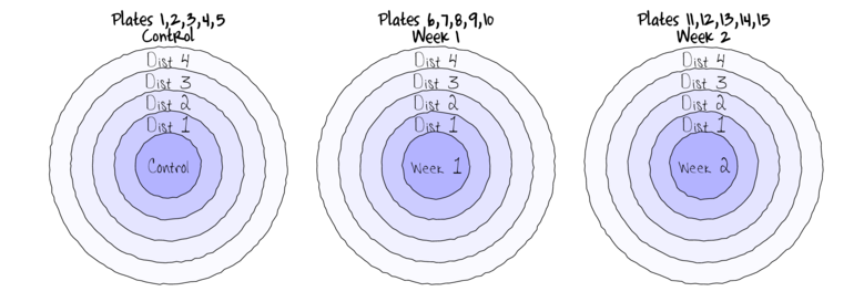
The Plates are the "random" groups. Within each Plate, all levels of the Distance factor occur (this is a within group factor). Each Plate can only be of one of the three levels of the Copper treatment. This is therefore a within group (nested) factor. Traditionally, this mixture of nested and randomized block design would be called a partly nested or split-plot design.
Notice that both the PLATE variable and the DIST variable contain only numbers. Make sure that you define both of these as factors (HINT)library(tidyverse) copper = copper %>% mutate(PLATE = factor(PLATE), DIST = factor(DIST))
- Perform exploratory data analysis
Show codeConclusions: there is some indication of a relationship between mean and variance (as suggested in boxplots). There is no evidence of a substantial interaction between the PLATES and DISTANCE within PLATES.
boxplot(WORMS ~ COPPER * DIST, copper)

ggplot(copper, aes(y = WORMS, x = DIST, fill = COPPER)) + geom_boxplot()

ggplot(copper, aes(y = WORMS, x = as.numeric(PLATE), color = COPPER)) + geom_line()

library(car) residualPlots(lm(WORMS ~ COPPER * DIST + PLATE, copper))

Test stat Pr(>|t|) COPPER NA NA DIST NA NA PLATE NA NA Tukey test 1.11 0.267
- Fit a range of candidate models
- random intercept model with COPPER and DIST (and their interaction) fixed component
- random intercept/slope (DIST) model with COPPER and DIST (and their interaction) fixed component
Show lme code## Since we only have a single replicate of each DIST within each PLATE, ## it does not make sense to model random intercept/slopes copper.lme = lme(WORMS ~ COPPER * DIST, random = ~1 | PLATE, data = copper, method = "REML", na.action = na.omit) copper.lme1 = lme(WORMS ~ COPPER * DIST, random = ~DIST | PLATE, data = copper, method = "REML", na.action = na.omit) # The newer nlmnb optimizer can be a bit flaky, try the BFGS optimizer # instead copper.lme2 = update(copper.lme1, random = ~DIST | PLATE, method = "REML", control = lmeControl(opt = "optim"), na.action = na.omit) anova(copper.lme1, copper.lme2)
Model df AIC BIC logLik copper.lme1 1 23 217.373 260.4106 -85.68648 copper.lme2 2 23 217.373 260.4106 -85.68648
Show lmer code## Since we only have a single replicate of each DIST within each PLATE, ## it does not make sense to model random intercept/slopes copper.lmer = lmer(WORMS ~ COPPER * DIST + (1 | PLATE), data = copper, REML = TRUE, na.action = na.omit)
Show glmmTMB code## Since we only have a single replicate of each DIST within each PLATE, ## it does not make sense to model random intercept/slopes copper.glmmTMB = glmmTMB(WORMS ~ COPPER * DIST + (1 | PLATE), data = copper, na.action = na.omit)
- Check the model diagnostics - validate the model
- Temporal and/or spatial autocorrelation. We do not have any information on the spatial or temporal collection of these data. Nevertheless, with only a small number of categories (and only two months), autocorrelation is not really an issue.
- Residual plots
Show lme codeplot(copper.lme)

qqnorm(resid(copper.lme)) qqline(resid(copper.lme))

copper.mod.dat = copper.lme$data ggplot(data = NULL) + geom_point(aes(y = resid(copper.lme, type = "normalized"), x = copper.mod.dat$COPPER))

ggplot(data = NULL) + geom_point(aes(y = resid(copper.lme, type = "normalized"), x = copper.mod.dat$DIST))

library(sjPlot) plot_grid(plot_model(copper.lme, type = "diag"))
 Show lmer code
qq.line = function(x) { # following four lines from base R's qqline() y <- quantile(x[!is.na(x)], c(0.25, 0.75)) x <- qnorm(c(0.25, 0.75)) slope <- diff(y)/diff(x) int <- y[1L] - slope * x[1L] return(c(int = int, slope = slope)) } plot(copper.lmer)

QQline = qq.line(resid(copper.lmer, type = "pearson", scale = TRUE)) ggplot(data = NULL, aes(sample = resid(copper.lmer, type = "pearson", scale = TRUE))) + stat_qq() + geom_abline(intercept = QQline[1], slope = QQline[2])

qqnorm(resid(copper.lmer)) qqline(resid(copper.lmer))

ggplot(data = NULL, aes(y = resid(copper.lmer, type = "pearson", scale = TRUE), x = fitted(copper.lmer))) + geom_point()

ggplot(data = NULL, aes(y = resid(copper.lmer, type = "pearson", scale = TRUE), x = copper.lmer@frame$COPPER)) + geom_point()

ggplot(data = NULL, aes(y = resid(copper.lmer, type = "pearson", scale = TRUE), x = copper.lmer@frame$DIST)) + geom_point()

library(sjPlot) plot_grid(plot_model(copper.lmer, type = "diag"))
 Show glmmTMB codeWhilst not ideal (there is some wedginess), the residual plots themselves appear acceptable.
qq.line = function(x) { # following four lines from base R's qqline() y <- quantile(x[!is.na(x)], c(0.25, 0.75)) x <- qnorm(c(0.25, 0.75)) slope <- diff(y)/diff(x) int <- y[1L] - slope * x[1L] return(c(int = int, slope = slope)) } ggplot(data = NULL, aes(y = resid(copper.glmmTMB, type = "pearson"), x = fitted(copper.glmmTMB))) + geom_point()

QQline = qq.line(resid(copper.glmmTMB, type = "pearson")) ggplot(data = NULL, aes(sample = resid(copper.glmmTMB, type = "pearson"))) + stat_qq() + geom_abline(intercept = QQline[1], slope = QQline[2])

ggplot(data = NULL, aes(y = resid(copper.glmmTMB, type = "pearson"), x = copper.glmmTMB$frame$COPPER)) + geom_point()

ggplot(data = NULL, aes(y = resid(copper.glmmTMB, type = "pearson"), x = copper.glmmTMB$frame$DIST)) + geom_point()

- Generate partial effects plots to assist with parameter interpretation
Show lme code
library(effects) plot(allEffects(copper.lme), multiline = TRUE, ci.style = "bars")

library(sjPlot) ## The following uses Effect (from effects package) and therefore does ## not account for the offset plot_model(copper.lme, type = "eff", terms = c("DIST", "COPPER"))

# don't add show.data=TRUE - this will add raw data not partial # residuals library(ggeffects) plot(ggeffect(copper.lmer, terms = c("DIST", "COPPER")))

# Ignoring uncertainty in random effects plot(ggpredict(copper.lme, terms = c("DIST", "COPPER")))
 Show lmer code
library(effects) plot(allEffects(copper.lmer, residuals = FALSE))

library(sjPlot) plot_model(copper.lmer, type = "eff", terms = c("DIST", "COPPER"))

# don't add show.data=TRUE - this will add raw data not partial # residuals library(ggeffects) plot(ggeffect(copper.lmer, terms = c("DIST", "COPPER")))
 Show glmmTMB code
library(ggeffects) # observation level effects averaged across margins p1 = ggaverage(copper.glmmTMB, terms = c("DIST", "COPPER")) ggplot(p1, aes(y = predicted, x = x, color = group, fill = group)) + geom_line()

p1 = ggpredict(copper.glmmTMB, terms = c("DIST", "COPPER")) ggplot(p1, aes(y = predicted, x = x, color = group, fill = group)) + geom_line() + geom_ribbon(aes(ymin = conf.low, ymax = conf.high), alpha = 0.3)

- Explore the parameter estimates for the 'best' model
Show lme code
summary(copper.lme)
Linear mixed-effects model fit by REML Data: copper AIC BIC logLik 218.2515 244.4483 -95.12575 Random effects: Formula: ~1 | PLATE (Intercept) Residual StdDev: 0.5599481 1.344162 Fixed effects: WORMS ~ COPPER * DIST Value Std.Error DF t-value p-value (Intercept) 10.85 0.6512008 36 16.661527 0.0000 COPPERWeek 1 -3.60 0.9209370 12 -3.909062 0.0021 COPPERWeek 2 -10.60 0.9209370 12 -11.510016 0.0000 DIST2 1.15 0.8501225 36 1.352746 0.1846 DIST3 1.55 0.8501225 36 1.823267 0.0766 DIST4 2.70 0.8501225 36 3.176013 0.0031 COPPERWeek 1:DIST2 -0.05 1.2022548 36 -0.041589 0.9671 COPPERWeek 2:DIST2 0.05 1.2022548 36 0.041589 0.9671 COPPERWeek 1:DIST3 -0.30 1.2022548 36 -0.249531 0.8044 COPPERWeek 2:DIST3 2.20 1.2022548 36 1.829895 0.0756 COPPERWeek 1:DIST4 0.05 1.2022548 36 0.041589 0.9671 COPPERWeek 2:DIST4 4.90 1.2022548 36 4.075675 0.0002 Correlation: (Intr) COPPERWk1 COPPERWk2 DIST2 DIST3 DIST4 COPPERW1:DIST2 COPPERW2:DIST2 COPPERWeek 1 -0.707 COPPERWeek 2 -0.707 0.500 DIST2 -0.653 0.462 0.462 DIST3 -0.653 0.462 0.462 0.500 DIST4 -0.653 0.462 0.462 0.500 0.500 COPPERWeek 1:DIST2 0.462 -0.653 -0.326 -0.707 -0.354 -0.354 COPPERWeek 2:DIST2 0.462 -0.326 -0.653 -0.707 -0.354 -0.354 0.500 COPPERWeek 1:DIST3 0.462 -0.653 -0.326 -0.354 -0.707 -0.354 0.500 0.250 COPPERWeek 2:DIST3 0.462 -0.326 -0.653 -0.354 -0.707 -0.354 0.250 0.500 COPPERWeek 1:DIST4 0.462 -0.653 -0.326 -0.354 -0.354 -0.707 0.500 0.250 COPPERWeek 2:DIST4 0.462 -0.326 -0.653 -0.354 -0.354 -0.707 0.250 0.500 COPPERW1:DIST3 COPPERW2:DIST3 COPPERW1:DIST4 COPPERWeek 1 COPPERWeek 2 DIST2 DIST3 DIST4 COPPERWeek 1:DIST2 COPPERWeek 2:DIST2 COPPERWeek 1:DIST3 COPPERWeek 2:DIST3 0.500 COPPERWeek 1:DIST4 0.500 0.250 COPPERWeek 2:DIST4 0.250 0.500 0.500 Standardized Within-Group Residuals: Min Q1 Med Q3 Max -1.61656136 -0.62651757 -0.09454227 0.46107961 2.51878597 Number of Observations: 60 Number of Groups: 15intervals(copper.lme)
Approximate 95% confidence intervals Fixed effects: lower est. upper (Intercept) 9.5293035 10.85 12.170696 COPPERWeek 1 -5.6065494 -3.60 -1.593451 COPPERWeek 2 -12.6065494 -10.60 -8.593451 DIST2 -0.5741284 1.15 2.874128 DIST3 -0.1741284 1.55 3.274128 DIST4 0.9758716 2.70 4.424128 COPPERWeek 1:DIST2 -2.4882857 -0.05 2.388286 COPPERWeek 2:DIST2 -2.3882857 0.05 2.488286 COPPERWeek 1:DIST3 -2.7382857 -0.30 2.138286 COPPERWeek 2:DIST3 -0.2382857 2.20 4.638286 COPPERWeek 1:DIST4 -2.3882857 0.05 2.488286 COPPERWeek 2:DIST4 2.4617143 4.90 7.338286 attr(,"label") [1] "Fixed effects:" Random Effects: Level: PLATE lower est. upper sd((Intercept)) 0.1995815 0.5599481 1.570997 Within-group standard error: lower est. upper 1.066945 1.344162 1.693405library(broom) tidy(copper.lme, effects = "fixed")
# A tibble: 12 x 5 term estimate std.error statistic p.value <chr> <dbl> <dbl> <dbl> <dbl> 1 (Intercept) 10.8 0.651 16.7 1.68e-18 2 COPPERWeek 1 -3.60 0.921 -3.91 2.08e- 3 3 COPPERWeek 2 -10.6 0.921 -11.5 7.68e- 8 4 DIST2 1.15 0.850 1.35 1.85e- 1 5 DIST3 1.55 0.850 1.82 7.66e- 2 6 DIST4 2.70 0.850 3.18 3.06e- 3 7 COPPERWeek 1:DIST2 -0.0500 1.20 -0.0416 9.67e- 1 8 COPPERWeek 2:DIST2 0.0500 1.20 0.0416 9.67e- 1 9 COPPERWeek 1:DIST3 -0.300 1.20 -0.250 8.04e- 1 10 COPPERWeek 2:DIST3 2.20 1.20 1.83 7.56e- 2 11 COPPERWeek 1:DIST4 0.0500 1.20 0.0416 9.67e- 1 12 COPPERWeek 2:DIST4 4.90 1.20 4.08 2.42e- 4
glance(copper.lme)
# A tibble: 1 x 5 sigma logLik AIC BIC deviance <dbl> <dbl> <dbl> <dbl> <lgl> 1 1.34 -95.1 218. 244. NA
anova(copper.lme, type = "marginal")
numDF denDF F-value p-value (Intercept) 1 36 277.60648 <.0001 COPPER 2 12 68.51191 <.0001 DIST 3 36 3.43615 0.0269 COPPER:DIST 6 36 4.92765 0.0009
Show lmer codesummary(copper.lmer)
Linear mixed model fit by REML t-tests use Satterthwaite approximations to degrees of freedom [ lmerMod] Formula: WORMS ~ COPPER * DIST + (1 | PLATE) Data: copper REML criterion at convergence: 190.3 Scaled residuals: Min 1Q Median 3Q Max -1.61656 -0.62652 -0.09454 0.46108 2.51879 Random effects: Groups Name Variance Std.Dev. PLATE (Intercept) 0.3135 0.5599 Residual 1.8068 1.3442 Number of obs: 60, groups: PLATE, 15 Fixed effects: Estimate Std. Error df t value Pr(>|t|) (Intercept) 10.8500 0.6512 45.0450 16.662 < 2e-16 *** COPPERWeek 1 -3.6000 0.9209 45.0450 -3.909 0.000309 *** COPPERWeek 2 -10.6000 0.9209 45.0450 -11.510 5.33e-15 *** DIST2 1.1500 0.8501 36.0000 1.353 0.184572 DIST3 1.5500 0.8501 36.0000 1.823 0.076575 . DIST4 2.7000 0.8501 36.0000 3.176 0.003058 ** COPPERWeek 1:DIST2 -0.0500 1.2023 36.0000 -0.042 0.967057 COPPERWeek 2:DIST2 0.0500 1.2023 36.0000 0.042 0.967057 COPPERWeek 1:DIST3 -0.3000 1.2023 36.0000 -0.250 0.804368 COPPERWeek 2:DIST3 2.2000 1.2023 36.0000 1.830 0.075556 . COPPERWeek 1:DIST4 0.0500 1.2023 36.0000 0.042 0.967057 COPPERWeek 2:DIST4 4.9000 1.2023 36.0000 4.076 0.000242 *** --- Signif. codes: 0 '***' 0.001 '**' 0.01 '*' 0.05 '.' 0.1 ' ' 1 Correlation of Fixed Effects: (Intr) COPPERWk1 COPPERWk2 DIST2 DIST3 DIST4 COPPERW1:DIST2 COPPERW2:DIST2 COPPERWeek1 -0.707 COPPERWeek2 -0.707 0.500 DIST2 -0.653 0.462 0.462 DIST3 -0.653 0.462 0.462 0.500 DIST4 -0.653 0.462 0.462 0.500 0.500 COPPERW1:DIST2 0.462 -0.653 -0.326 -0.707 -0.354 -0.354 COPPERW2:DIST2 0.462 -0.326 -0.653 -0.707 -0.354 -0.354 0.500 COPPERW1:DIST3 0.462 -0.653 -0.326 -0.354 -0.707 -0.354 0.500 0.250 COPPERW2:DIST3 0.462 -0.326 -0.653 -0.354 -0.707 -0.354 0.250 0.500 COPPERW1:DIST4 0.462 -0.653 -0.326 -0.354 -0.354 -0.707 0.500 0.250 COPPERW2:DIST4 0.462 -0.326 -0.653 -0.354 -0.354 -0.707 0.250 0.500 COPPERW1:DIST3 COPPERW2:DIST3 COPPERW1:DIST4 COPPERWeek1 COPPERWeek2 DIST2 DIST3 DIST4 COPPERW1:DIST2 COPPERW2:DIST2 COPPERW1:DIST3 COPPERW2:DIST3 0.500 COPPERW1:DIST4 0.500 0.250 COPPERW2:DIST4 0.250 0.500 0.500confint(copper.lmer)
2.5 % 97.5 % .sig01 0.0000000 1.012975 .sigma 0.9909403 1.500906 (Intercept) 9.6885181 12.011482 COPPERWeek 1 -5.2425834 -1.957417 COPPERWeek 2 -12.2425834 -8.957417 DIST2 -0.3762398 2.672147 DIST3 0.5900189 2.825714 DIST4 1.7400189 3.975714 COPPERWeek 1:DIST2 -1.4076183 1.754131 COPPERWeek 2:DIST2 -1.3076183 1.854131 COPPERWeek 1:DIST3 -1.6576183 1.504131 COPPERWeek 2:DIST3 0.8423817 4.004131 COPPERWeek 1:DIST4 -1.3076183 1.854131 COPPERWeek 2:DIST4 2.8005588 6.704342
library(broom) tidy(copper.lmer, effects = "fixed", conf.int = TRUE)
# A tibble: 12 x 6 term estimate std.error statistic conf.low conf.high <chr> <dbl> <dbl> <dbl> <dbl> <dbl> 1 (Intercept) 10.9 0.651 16.7 9.57 12.1 2 COPPERWeek 1 -3.60 0.921 -3.91 -5.41 -1.79 3 COPPERWeek 2 -10.6 0.921 -11.5 -12.4 -8.79 4 DIST2 1.15 0.850 1.35 -0.516 2.82 5 DIST3 1.55 0.850 1.82 -0.116 3.22 6 DIST4 2.70 0.850 3.18 1.03 4.37 7 COPPERWeek 1:DIST2 -0.0500 1.20 -0.0416 -2.41 2.31 8 COPPERWeek 2:DIST2 0.0500 1.20 0.0416 -2.31 2.41 9 COPPERWeek 1:DIST3 -0.300 1.20 -0.250 -2.66 2.06 10 COPPERWeek 2:DIST3 2.20 1.20 1.83 -0.156 4.56 11 COPPERWeek 1:DIST4 0.0500 1.20 0.0416 -2.31 2.41 12 COPPERWeek 2:DIST4 4.90 1.20 4.08 2.54 7.26
glance(copper.lmer)
# A tibble: 1 x 6 sigma logLik AIC BIC deviance df.residual <dbl> <dbl> <dbl> <dbl> <dbl> <int> 1 1.34 -95.1 218. 248. 200. 46
anova(copper.lmer, type = "marginal")
Analysis of Variance Table Df Sum Sq Mean Sq F value COPPER 2 462.61 231.305 128.0214 DIST 3 153.80 51.268 28.3753 COPPER:DIST 6 53.42 8.903 4.9276## If you cant live without p-values... library(lmerTest) copper.lmer <- update(copper.lmer) summary(copper.lmer)
Linear mixed model fit by REML ['lmerMod'] Formula: WORMS ~ COPPER * DIST + (1 | PLATE) Data: copper REML criterion at convergence: 190.3 Scaled residuals: Min 1Q Median 3Q Max -1.61656 -0.62652 -0.09454 0.46108 2.51879 Random effects: Groups Name Variance Std.Dev. PLATE (Intercept) 0.3135 0.5599 Residual 1.8068 1.3442 Number of obs: 60, groups: PLATE, 15 Fixed effects: Estimate Std. Error t value (Intercept) 10.8500 0.6512 16.662 COPPERWeek 1 -3.6000 0.9209 -3.909 COPPERWeek 2 -10.6000 0.9209 -11.510 DIST2 1.1500 0.8501 1.353 DIST3 1.5500 0.8501 1.823 DIST4 2.7000 0.8501 3.176 COPPERWeek 1:DIST2 -0.0500 1.2023 -0.042 COPPERWeek 2:DIST2 0.0500 1.2023 0.042 COPPERWeek 1:DIST3 -0.3000 1.2023 -0.250 COPPERWeek 2:DIST3 2.2000 1.2023 1.830 COPPERWeek 1:DIST4 0.0500 1.2023 0.042 COPPERWeek 2:DIST4 4.9000 1.2023 4.076 Correlation of Fixed Effects: (Intr) COPPERWk1 COPPERWk2 DIST2 DIST3 DIST4 COPPERW1:DIST2 COPPERW2:DIST2 COPPERWeek1 -0.707 COPPERWeek2 -0.707 0.500 DIST2 -0.653 0.462 0.462 DIST3 -0.653 0.462 0.462 0.500 DIST4 -0.653 0.462 0.462 0.500 0.500 COPPERW1:DIST2 0.462 -0.653 -0.326 -0.707 -0.354 -0.354 COPPERW2:DIST2 0.462 -0.326 -0.653 -0.707 -0.354 -0.354 0.500 COPPERW1:DIST3 0.462 -0.653 -0.326 -0.354 -0.707 -0.354 0.500 0.250 COPPERW2:DIST3 0.462 -0.326 -0.653 -0.354 -0.707 -0.354 0.250 0.500 COPPERW1:DIST4 0.462 -0.653 -0.326 -0.354 -0.354 -0.707 0.500 0.250 COPPERW2:DIST4 0.462 -0.326 -0.653 -0.354 -0.354 -0.707 0.250 0.500 COPPERW1:DIST3 COPPERW2:DIST3 COPPERW1:DIST4 COPPERWeek1 COPPERWeek2 DIST2 DIST3 DIST4 COPPERW1:DIST2 COPPERW2:DIST2 COPPERW1:DIST3 COPPERW2:DIST3 0.500 COPPERW1:DIST4 0.500 0.250 COPPERW2:DIST4 0.250 0.500 0.500anova(copper.lmer) # Satterthwaite denominator df method
Analysis of Variance Table Df Sum Sq Mean Sq F value COPPER 2 462.61 231.305 128.0214 DIST 3 153.80 51.268 28.3753 COPPER:DIST 6 53.42 8.903 4.9276anova(copper.lmer, ddf = "Kenward-Roger")
Analysis of Variance Table Df Sum Sq Mean Sq F value COPPER 2 462.61 231.305 128.0214 DIST 3 153.80 51.268 28.3753 COPPER:DIST 6 53.42 8.903 4.9276Show glmmTMB codeConclusions:summary(copper.glmmTMB)
Family: gaussian ( identity ) Formula: WORMS ~ COPPER * DIST + (1 | PLATE) Data: copper AIC BIC logLik deviance df.resid 228.3 257.6 -100.1 200.3 46 Random effects: Conditional model: Groups Name Variance Std.Dev. PLATE (Intercept) 0.2508 0.5008 Residual 1.4454 1.2023 Number of obs: 60, groups: PLATE, 15 Dispersion estimate for gaussian family (sigma^2): 1.45 Conditional model: Estimate Std. Error z value Pr(>|z|) (Intercept) 10.8500 0.5825 18.628 < 2e-16 *** COPPERWeek 1 -3.6000 0.8237 -4.370 1.24e-05 *** COPPERWeek 2 -10.6000 0.8237 -12.869 < 2e-16 *** DIST2 1.1500 0.7604 1.512 0.130428 DIST3 1.5500 0.7604 2.038 0.041503 * DIST4 2.7000 0.7604 3.551 0.000384 *** COPPERWeek 1:DIST2 -0.0500 1.0753 -0.046 0.962914 COPPERWeek 2:DIST2 0.0500 1.0753 0.046 0.962913 COPPERWeek 1:DIST3 -0.3000 1.0753 -0.279 0.780257 COPPERWeek 2:DIST3 2.2000 1.0753 2.046 0.040768 * COPPERWeek 1:DIST4 0.0500 1.0753 0.046 0.962913 COPPERWeek 2:DIST4 4.9000 1.0753 4.557 5.20e-06 *** --- Signif. codes: 0 '***' 0.001 '**' 0.01 '*' 0.05 '.' 0.1 ' ' 1confint(copper.glmmTMB)
2.5 % 97.5 % Estimate cond.(Intercept) 9.70841619 11.991585 10.85000043 cond.COPPERWeek 1 -5.21444466 -1.985557 -3.60000075 cond.COPPERWeek 2 -12.21444430 -8.985556 -10.60000038 cond.DIST2 -0.34030361 2.640302 1.14999938 cond.DIST3 0.05969647 3.040302 1.54999946 cond.DIST4 1.20969654 4.190303 2.69999954 cond.COPPERWeek 1:DIST2 -2.15760602 2.057607 -0.04999931 cond.COPPERWeek 2:DIST2 -2.05760591 2.157607 0.05000079 cond.COPPERWeek 1:DIST3 -2.40760598 1.807607 -0.29999927 cond.COPPERWeek 2:DIST3 0.09239378 4.307607 2.20000049 cond.COPPERWeek 1:DIST4 -2.05760600 2.157607 0.05000070 cond.COPPERWeek 2:DIST4 2.79239343 7.007607 4.90000013 cond.Std.Dev.PLATE.(Intercept) 0.19905933 1.260093 0.50083249 sigma 0.97784941 1.478158 1.20225471
- there is evidence of an interaction between copper treatment and distance from source (middle of the plate)
- The distance patterns of worm density on Control copper treatment plates differs from that of the Week2 treatment, yet not the Week1 treatment.
- Explore the pairwise comparisons of the copper treatment using a Tukey's tests separate
for each distance.
Show lme code
## emmeans ------------------------------------------- library(emmeans) emmeans(copper.lme, pairwise ~ COPPER | DIST)
$emmeans DIST = 1: COPPER emmean SE df lower.CL upper.CL control 10.85 0.6512008 14 9.45331315 12.246687 Week 1 7.25 0.6512008 12 5.83115529 8.668845 Week 2 0.25 0.6512008 12 -1.16884471 1.668845 DIST = 2: COPPER emmean SE df lower.CL upper.CL control 12.00 0.6512008 14 10.60331315 13.396687 Week 1 8.35 0.6512008 12 6.93115529 9.768845 Week 2 1.45 0.6512008 12 0.03115529 2.868845 DIST = 3: COPPER emmean SE df lower.CL upper.CL control 12.40 0.6512008 14 11.00331315 13.796687 Week 1 8.50 0.6512008 12 7.08115529 9.918845 Week 2 4.00 0.6512008 12 2.58115529 5.418845 DIST = 4: COPPER emmean SE df lower.CL upper.CL control 13.55 0.6512008 14 12.15331315 14.946687 Week 1 10.00 0.6512008 12 8.58115529 11.418845 Week 2 7.85 0.6512008 12 6.43115529 9.268845 Degrees-of-freedom method: containment Confidence level used: 0.95 $contrasts DIST = 1: contrast estimate SE df t.ratio p.value control - Week 1 3.60 0.920937 12 3.909 0.0054 control - Week 2 10.60 0.920937 12 11.510 <.0001 Week 1 - Week 2 7.00 0.920937 12 7.601 <.0001 DIST = 2: contrast estimate SE df t.ratio p.value control - Week 1 3.65 0.920937 12 3.963 0.0049 control - Week 2 10.55 0.920937 12 11.456 <.0001 Week 1 - Week 2 6.90 0.920937 12 7.492 <.0001 DIST = 3: contrast estimate SE df t.ratio p.value control - Week 1 3.90 0.920937 12 4.235 0.0031 control - Week 2 8.40 0.920937 12 9.121 <.0001 Week 1 - Week 2 4.50 0.920937 12 4.886 0.0010 DIST = 4: contrast estimate SE df t.ratio p.value control - Week 1 3.55 0.920937 12 3.855 0.0060 control - Week 2 5.70 0.920937 12 6.189 0.0001 Week 1 - Week 2 2.15 0.920937 12 2.335 0.0890 P value adjustment: tukey method for comparing a family of 3 estimates
confint(emmeans(copper.lme, pairwise ~ COPPER | DIST))
$emmeans DIST = 1: COPPER emmean SE df lower.CL upper.CL control 10.85 0.6512008 14 9.45331315 12.246687 Week 1 7.25 0.6512008 12 5.83115529 8.668845 Week 2 0.25 0.6512008 12 -1.16884471 1.668845 DIST = 2: COPPER emmean SE df lower.CL upper.CL control 12.00 0.6512008 14 10.60331315 13.396687 Week 1 8.35 0.6512008 12 6.93115529 9.768845 Week 2 1.45 0.6512008 12 0.03115529 2.868845 DIST = 3: COPPER emmean SE df lower.CL upper.CL control 12.40 0.6512008 14 11.00331315 13.796687 Week 1 8.50 0.6512008 12 7.08115529 9.918845 Week 2 4.00 0.6512008 12 2.58115529 5.418845 DIST = 4: COPPER emmean SE df lower.CL upper.CL control 13.55 0.6512008 14 12.15331315 14.946687 Week 1 10.00 0.6512008 12 8.58115529 11.418845 Week 2 7.85 0.6512008 12 6.43115529 9.268845 Degrees-of-freedom method: containment Confidence level used: 0.95 $contrasts DIST = 1: contrast estimate SE df lower.CL upper.CL control - Week 1 3.60 0.920937 12 1.1430656 6.056934 control - Week 2 10.60 0.920937 12 8.1430656 13.056934 Week 1 - Week 2 7.00 0.920937 12 4.5430656 9.456934 DIST = 2: contrast estimate SE df lower.CL upper.CL control - Week 1 3.65 0.920937 12 1.1930656 6.106934 control - Week 2 10.55 0.920937 12 8.0930656 13.006934 Week 1 - Week 2 6.90 0.920937 12 4.4430656 9.356934 DIST = 3: contrast estimate SE df lower.CL upper.CL control - Week 1 3.90 0.920937 12 1.4430656 6.356934 control - Week 2 8.40 0.920937 12 5.9430656 10.856934 Week 1 - Week 2 4.50 0.920937 12 2.0430656 6.956934 DIST = 4: contrast estimate SE df lower.CL upper.CL control - Week 1 3.55 0.920937 12 1.0930656 6.006934 control - Week 2 5.70 0.920937 12 3.2430656 8.156934 Week 1 - Week 2 2.15 0.920937 12 -0.3069344 4.606934 Confidence level used: 0.95 Conf-level adjustment: tukey method for comparing a family of 3 estimates
## glht and emmeans -------------------------------------------- summary(glht(copper.lme, linfct = lsm(pairwise ~ COPPER | DIST)))
$`DIST = 1` Simultaneous Tests for General Linear Hypotheses Fit: lme.formula(fixed = WORMS ~ COPPER * DIST, data = copper, random = ~1 | PLATE, method = "REML", na.action = na.omit) Linear Hypotheses: Estimate Std. Error t value Pr(>|t|) control - Week 1 == 0 3.6000 0.9209 3.909 0.00533 ** control - Week 2 == 0 10.6000 0.9209 11.510 < 0.001 *** Week 1 - Week 2 == 0 7.0000 0.9209 7.601 < 0.001 *** --- Signif. codes: 0 '***' 0.001 '**' 0.01 '*' 0.05 '.' 0.1 ' ' 1 (Adjusted p values reported -- single-step method) $`DIST = 2` Simultaneous Tests for General Linear Hypotheses Fit: lme.formula(fixed = WORMS ~ COPPER * DIST, data = copper, random = ~1 | PLATE, method = "REML", na.action = na.omit) Linear Hypotheses: Estimate Std. Error t value Pr(>|t|) control - Week 1 == 0 3.6500 0.9209 3.963 0.00491 ** control - Week 2 == 0 10.5500 0.9209 11.456 < 0.001 *** Week 1 - Week 2 == 0 6.9000 0.9209 7.492 < 0.001 *** --- Signif. codes: 0 '***' 0.001 '**' 0.01 '*' 0.05 '.' 0.1 ' ' 1 (Adjusted p values reported -- single-step method) $`DIST = 3` Simultaneous Tests for General Linear Hypotheses Fit: lme.formula(fixed = WORMS ~ COPPER * DIST, data = copper, random = ~1 | PLATE, method = "REML", na.action = na.omit) Linear Hypotheses: Estimate Std. Error t value Pr(>|t|) control - Week 1 == 0 3.9000 0.9209 4.235 0.00293 ** control - Week 2 == 0 8.4000 0.9209 9.121 < 0.001 *** Week 1 - Week 2 == 0 4.5000 0.9209 4.886 < 0.001 *** --- Signif. codes: 0 '***' 0.001 '**' 0.01 '*' 0.05 '.' 0.1 ' ' 1 (Adjusted p values reported -- single-step method) $`DIST = 4` Simultaneous Tests for General Linear Hypotheses Fit: lme.formula(fixed = WORMS ~ COPPER * DIST, data = copper, random = ~1 | PLATE, method = "REML", na.action = na.omit) Linear Hypotheses: Estimate Std. Error t value Pr(>|t|) control - Week 1 == 0 3.5500 0.9209 3.855 0.00589 ** control - Week 2 == 0 5.7000 0.9209 6.189 < 0.001 *** Week 1 - Week 2 == 0 2.1500 0.9209 2.335 0.08895 . --- Signif. codes: 0 '***' 0.001 '**' 0.01 '*' 0.05 '.' 0.1 ' ' 1 (Adjusted p values reported -- single-step method)confint(glht(copper.lme, linfct = lsm(pairwise ~ COPPER | DIST)))
$`DIST = 1` Simultaneous Confidence Intervals Fit: lme.formula(fixed = WORMS ~ COPPER * DIST, data = copper, random = ~1 | PLATE, method = "REML", na.action = na.omit) Quantile = 2.667 95% family-wise confidence level Linear Hypotheses: Estimate lwr upr control - Week 1 == 0 3.6000 1.1439 6.0561 control - Week 2 == 0 10.6000 8.1439 13.0561 Week 1 - Week 2 == 0 7.0000 4.5439 9.4561 $`DIST = 2` Simultaneous Confidence Intervals Fit: lme.formula(fixed = WORMS ~ COPPER * DIST, data = copper, random = ~1 | PLATE, method = "REML", na.action = na.omit) Quantile = 2.667 95% family-wise confidence level Linear Hypotheses: Estimate lwr upr control - Week 1 == 0 3.6500 1.1938 6.1062 control - Week 2 == 0 10.5500 8.0938 13.0062 Week 1 - Week 2 == 0 6.9000 4.4438 9.3562 $`DIST = 3` Simultaneous Confidence Intervals Fit: lme.formula(fixed = WORMS ~ COPPER * DIST, data = copper, random = ~1 | PLATE, method = "REML", na.action = na.omit) Quantile = 2.6667 95% family-wise confidence level Linear Hypotheses: Estimate lwr upr control - Week 1 == 0 3.9000 1.4441 6.3559 control - Week 2 == 0 8.4000 5.9441 10.8559 Week 1 - Week 2 == 0 4.5000 2.0441 6.9559 $`DIST = 4` Simultaneous Confidence Intervals Fit: lme.formula(fixed = WORMS ~ COPPER * DIST, data = copper, random = ~1 | PLATE, method = "REML", na.action = na.omit) Quantile = 2.6682 95% family-wise confidence level Linear Hypotheses: Estimate lwr upr control - Week 1 == 0 3.5500 1.0928 6.0072 control - Week 2 == 0 5.7000 3.2428 8.1572 Week 1 - Week 2 == 0 2.1500 -0.3072 4.6072## or manually ------------------------------------------------- Note, ## this does not correct for family-wise error rate. newdata = with(copper, expand.grid(COPPER = levels(COPPER), DIST = levels(DIST))) Xmat = model.matrix(~COPPER * DIST, data = newdata) coefs = fixef(copper.lme) Xmat.split = split.data.frame(Xmat, f = newdata$DIST) tuk.mat <- contrMat(n = table(levels(newdata$COPPER)), type = "Tukey") lapply(Xmat.split, function(x) { Xmat = tuk.mat %*% x fit = as.vector(coefs %*% t(Xmat)) se = sqrt(diag(Xmat %*% vcov(copper.lme) %*% t(Xmat))) Q = qt(0.975, copper.lme$fixDF$terms["COPPER"]) # Q=1.96 data.frame(fit = fit, lower = fit - Q * se, upper = fit + Q * se) })
$`1` fit lower upper Week 1 - control -3.6 -5.606549 -1.593451 Week 2 - control -10.6 -12.606549 -8.593451 Week 2 - Week 1 -7.0 -9.006549 -4.993451 $`2` fit lower upper Week 1 - control -3.65 -5.656549 -1.643451 Week 2 - control -10.55 -12.556549 -8.543451 Week 2 - Week 1 -6.90 -8.906549 -4.893451 $`3` fit lower upper Week 1 - control -3.9 -5.906549 -1.893451 Week 2 - control -8.4 -10.406549 -6.393451 Week 2 - Week 1 -4.5 -6.506549 -2.493451 $`4` fit lower upper Week 1 - control -3.55 -5.556549 -1.5434506 Week 2 - control -5.70 -7.706549 -3.6934506 Week 2 - Week 1 -2.15 -4.156549 -0.1434506Show lmer code## emmeans ------------------------------------------- library(emmeans) emmeans(copper.lmer, pairwise ~ COPPER | DIST)
$emmeans DIST = 1: COPPER emmean SE df lower.CL upper.CL control 10.85 0.6512008 45.04 9.5384504 12.16155 Week 1 7.25 0.6512008 45.04 5.9384504 8.56155 Week 2 0.25 0.6512008 45.04 -1.0615496 1.56155 DIST = 2: COPPER emmean SE df lower.CL upper.CL control 12.00 0.6512008 45.04 10.6884504 13.31155 Week 1 8.35 0.6512008 45.04 7.0384504 9.66155 Week 2 1.45 0.6512008 45.04 0.1384504 2.76155 DIST = 3: COPPER emmean SE df lower.CL upper.CL control 12.40 0.6512008 45.04 11.0884504 13.71155 Week 1 8.50 0.6512008 45.04 7.1884504 9.81155 Week 2 4.00 0.6512008 45.04 2.6884504 5.31155 DIST = 4: COPPER emmean SE df lower.CL upper.CL control 13.55 0.6512008 45.04 12.2384504 14.86155 Week 1 10.00 0.6512008 45.04 8.6884504 11.31155 Week 2 7.85 0.6512008 45.04 6.5384504 9.16155 Degrees-of-freedom method: kenward-roger Confidence level used: 0.95 $contrasts DIST = 1: contrast estimate SE df t.ratio p.value control - Week 1 3.60 0.920937 45.04 3.909 0.0009 control - Week 2 10.60 0.920937 45.04 11.510 <.0001 Week 1 - Week 2 7.00 0.920937 45.04 7.601 <.0001 DIST = 2: contrast estimate SE df t.ratio p.value control - Week 1 3.65 0.920937 45.04 3.963 0.0008 control - Week 2 10.55 0.920937 45.04 11.456 <.0001 Week 1 - Week 2 6.90 0.920937 45.04 7.492 <.0001 DIST = 3: contrast estimate SE df t.ratio p.value control - Week 1 3.90 0.920937 45.04 4.235 0.0003 control - Week 2 8.40 0.920937 45.04 9.121 <.0001 Week 1 - Week 2 4.50 0.920937 45.04 4.886 <.0001 DIST = 4: contrast estimate SE df t.ratio p.value control - Week 1 3.55 0.920937 45.04 3.855 0.0010 control - Week 2 5.70 0.920937 45.04 6.189 <.0001 Week 1 - Week 2 2.15 0.920937 45.04 2.335 0.0612 P value adjustment: tukey method for comparing a family of 3 estimates
confint(emmeans(copper.lmer, pairwise ~ COPPER | DIST))
$emmeans DIST = 1: COPPER emmean SE df lower.CL upper.CL control 10.85 0.6512008 45.04 9.5384504 12.16155 Week 1 7.25 0.6512008 45.04 5.9384504 8.56155 Week 2 0.25 0.6512008 45.04 -1.0615496 1.56155 DIST = 2: COPPER emmean SE df lower.CL upper.CL control 12.00 0.6512008 45.04 10.6884504 13.31155 Week 1 8.35 0.6512008 45.04 7.0384504 9.66155 Week 2 1.45 0.6512008 45.04 0.1384504 2.76155 DIST = 3: COPPER emmean SE df lower.CL upper.CL control 12.40 0.6512008 45.04 11.0884504 13.71155 Week 1 8.50 0.6512008 45.04 7.1884504 9.81155 Week 2 4.00 0.6512008 45.04 2.6884504 5.31155 DIST = 4: COPPER emmean SE df lower.CL upper.CL control 13.55 0.6512008 45.04 12.2384504 14.86155 Week 1 10.00 0.6512008 45.04 8.6884504 11.31155 Week 2 7.85 0.6512008 45.04 6.5384504 9.16155 Degrees-of-freedom method: kenward-roger Confidence level used: 0.95 $contrasts DIST = 1: contrast estimate SE df lower.CL upper.CL control - Week 1 3.60 0.920937 45.04 1.36808009 5.83192 control - Week 2 10.60 0.920937 45.04 8.36808009 12.83192 Week 1 - Week 2 7.00 0.920937 45.04 4.76808009 9.23192 DIST = 2: contrast estimate SE df lower.CL upper.CL control - Week 1 3.65 0.920937 45.04 1.41808009 5.88192 control - Week 2 10.55 0.920937 45.04 8.31808009 12.78192 Week 1 - Week 2 6.90 0.920937 45.04 4.66808009 9.13192 DIST = 3: contrast estimate SE df lower.CL upper.CL control - Week 1 3.90 0.920937 45.04 1.66808009 6.13192 control - Week 2 8.40 0.920937 45.04 6.16808009 10.63192 Week 1 - Week 2 4.50 0.920937 45.04 2.26808009 6.73192 DIST = 4: contrast estimate SE df lower.CL upper.CL control - Week 1 3.55 0.920937 45.04 1.31808009 5.78192 control - Week 2 5.70 0.920937 45.04 3.46808009 7.93192 Week 1 - Week 2 2.15 0.920937 45.04 -0.08191991 4.38192 Confidence level used: 0.95 Conf-level adjustment: tukey method for comparing a family of 3 estimates
## glht and emmeans -------------------------------------------- summary(glht(copper.lmer, linfct = lsm(pairwise ~ COPPER | DIST)))
$`DIST = 1` Simultaneous Tests for General Linear Hypotheses Fit: lme4::lmer(formula = WORMS ~ COPPER * DIST + (1 | PLATE), data = copper, REML = TRUE, na.action = na.omit) Linear Hypotheses: Estimate Std. Error t value Pr(>|t|) control - Week 1 == 0 3.6000 0.9209 3.909 0.000908 *** control - Week 2 == 0 10.6000 0.9209 11.510 < 1e-04 *** Week 1 - Week 2 == 0 7.0000 0.9209 7.601 < 1e-04 *** --- Signif. codes: 0 '***' 0.001 '**' 0.01 '*' 0.05 '.' 0.1 ' ' 1 (Adjusted p values reported -- single-step method) $`DIST = 2` Simultaneous Tests for General Linear Hypotheses Fit: lme4::lmer(formula = WORMS ~ COPPER * DIST + (1 | PLATE), data = copper, REML = TRUE, na.action = na.omit) Linear Hypotheses: Estimate Std. Error t value Pr(>|t|) control - Week 1 == 0 3.6500 0.9209 3.963 <0.001 *** control - Week 2 == 0 10.5500 0.9209 11.456 <0.001 *** Week 1 - Week 2 == 0 6.9000 0.9209 7.492 <0.001 *** --- Signif. codes: 0 '***' 0.001 '**' 0.01 '*' 0.05 '.' 0.1 ' ' 1 (Adjusted p values reported -- single-step method) $`DIST = 3` Simultaneous Tests for General Linear Hypotheses Fit: lme4::lmer(formula = WORMS ~ COPPER * DIST + (1 | PLATE), data = copper, REML = TRUE, na.action = na.omit) Linear Hypotheses: Estimate Std. Error t value Pr(>|t|) control - Week 1 == 0 3.9000 0.9209 4.235 0.000302 *** control - Week 2 == 0 8.4000 0.9209 9.121 < 1e-04 *** Week 1 - Week 2 == 0 4.5000 0.9209 4.886 < 1e-04 *** --- Signif. codes: 0 '***' 0.001 '**' 0.01 '*' 0.05 '.' 0.1 ' ' 1 (Adjusted p values reported -- single-step method) $`DIST = 4` Simultaneous Tests for General Linear Hypotheses Fit: lme4::lmer(formula = WORMS ~ COPPER * DIST + (1 | PLATE), data = copper, REML = TRUE, na.action = na.omit) Linear Hypotheses: Estimate Std. Error t value Pr(>|t|) control - Week 1 == 0 3.5500 0.9209 3.855 0.00113 ** control - Week 2 == 0 5.7000 0.9209 6.189 < 0.001 *** Week 1 - Week 2 == 0 2.1500 0.9209 2.335 0.06115 . --- Signif. codes: 0 '***' 0.001 '**' 0.01 '*' 0.05 '.' 0.1 ' ' 1 (Adjusted p values reported -- single-step method)confint(glht(copper.lmer, linfct = lsm(pairwise ~ COPPER | DIST)))
$`DIST = 1` Simultaneous Confidence Intervals Fit: lme4::lmer(formula = WORMS ~ COPPER * DIST + (1 | PLATE), data = copper, REML = TRUE, na.action = na.omit) Quantile = 2.4233 95% family-wise confidence level Linear Hypotheses: Estimate lwr upr control - Week 1 == 0 3.6000 1.3683 5.8317 control - Week 2 == 0 10.6000 8.3683 12.8317 Week 1 - Week 2 == 0 7.0000 4.7683 9.2317 $`DIST = 2` Simultaneous Confidence Intervals Fit: lme4::lmer(formula = WORMS ~ COPPER * DIST + (1 | PLATE), data = copper, REML = TRUE, na.action = na.omit) Quantile = 2.4239 95% family-wise confidence level Linear Hypotheses: Estimate lwr upr control - Week 1 == 0 3.6500 1.4177 5.8823 control - Week 2 == 0 10.5500 8.3177 12.7823 Week 1 - Week 2 == 0 6.9000 4.6677 9.1323 $`DIST = 3` Simultaneous Confidence Intervals Fit: lme4::lmer(formula = WORMS ~ COPPER * DIST + (1 | PLATE), data = copper, REML = TRUE, na.action = na.omit) Quantile = 2.4233 95% family-wise confidence level Linear Hypotheses: Estimate lwr upr control - Week 1 == 0 3.9000 1.6683 6.1317 control - Week 2 == 0 8.4000 6.1683 10.6317 Week 1 - Week 2 == 0 4.5000 2.2683 6.7317 $`DIST = 4` Simultaneous Confidence Intervals Fit: lme4::lmer(formula = WORMS ~ COPPER * DIST + (1 | PLATE), data = copper, REML = TRUE, na.action = na.omit) Quantile = 2.4241 95% family-wise confidence level Linear Hypotheses: Estimate lwr upr control - Week 1 == 0 3.55000 1.31755 5.78245 control - Week 2 == 0 5.70000 3.46755 7.93245 Week 1 - Week 2 == 0 2.15000 -0.08245 4.38245## or manually ------------------------------------------------- Note, ## this does not correct for family-wise error rate. newdata = with(copper, expand.grid(COPPER = levels(COPPER), DIST = levels(DIST))) Xmat = model.matrix(~COPPER * DIST, data = newdata) coefs = fixef(copper.lmer) Xmat.split = split.data.frame(Xmat, f = newdata$DIST) tuk.mat <- contrMat(n = table(levels(newdata$COPPER)), type = "Tukey") lapply(Xmat.split, function(x) { Xmat = tuk.mat %*% x fit = as.vector(coefs %*% t(Xmat)) se = sqrt(diag(Xmat %*% vcov(copper.lmer) %*% t(Xmat))) Q = qt(0.975, lmerTest::calcSatterth(copper.lmer, x)$denom) # Q=1.96 data.frame(fit = fit, lower = fit - Q * se, upper = fit + Q * se) })
$`1` fit lower upper 1 -3.6 -5.454811 -1.745189 2 -10.6 -12.454811 -8.745189 3 -7.0 -8.854811 -5.145189 $`2` fit lower upper 1 -3.65 -5.504811 -1.795189 2 -10.55 -12.404811 -8.695189 3 -6.90 -8.754811 -5.045189 $`3` fit lower upper 1 -3.9 -5.754811 -2.045189 2 -8.4 -10.254811 -6.545189 3 -4.5 -6.354811 -2.645189 $`4` fit lower upper 1 -3.55 -5.404811 -1.6951888 2 -5.70 -7.554811 -3.8451888 3 -2.15 -4.004811 -0.2951888Show glmmTMB code## emmeans ------------------------------------------- library(emmeans) emmeans(copper.glmmTMB, pairwise ~ COPPER | DIST)
$emmeans DIST = 1: COPPER emmean SE df lower.CL upper.CL control 10.8500004 0.5824516 46 9.6775861 12.022415 Week 1 7.2499997 0.5824516 46 6.0775853 8.422414 Week 2 0.2500001 0.5824516 46 -0.9224143 1.422414 DIST = 2: COPPER emmean SE df lower.CL upper.CL control 11.9999998 0.5824516 46 10.8275855 13.172414 Week 1 8.3499998 0.5824516 46 7.1775854 9.522414 Week 2 1.4500002 0.5824516 46 0.2775859 2.622415 DIST = 3: COPPER emmean SE df lower.CL upper.CL control 12.3999999 0.5824516 46 11.2275855 13.572414 Week 1 8.4999999 0.5824516 46 7.3275855 9.672414 Week 2 4.0000000 0.5824516 46 2.8275857 5.172414 DIST = 4: COPPER emmean SE df lower.CL upper.CL control 13.5500000 0.5824516 46 12.3775856 14.722414 Week 1 9.9999999 0.5824516 46 8.8275856 11.172414 Week 2 7.8499997 0.5824516 46 6.6775854 9.022414 Confidence level used: 0.95 $contrasts DIST = 1: contrast estimate SE df t.ratio p.value control - Week 1 3.600001 0.823711 46 4.370 0.0002 control - Week 2 10.600000 0.823711 46 12.869 <.0001 Week 1 - Week 2 7.000000 0.823711 46 8.498 <.0001 DIST = 2: contrast estimate SE df t.ratio p.value control - Week 1 3.650000 0.823711 46 4.431 0.0002 control - Week 2 10.550000 0.823711 46 12.808 <.0001 Week 1 - Week 2 6.900000 0.823711 46 8.377 <.0001 DIST = 3: contrast estimate SE df t.ratio p.value control - Week 1 3.900000 0.823711 46 4.735 0.0001 control - Week 2 8.400000 0.823711 46 10.198 <.0001 Week 1 - Week 2 4.500000 0.823711 46 5.463 <.0001 DIST = 4: contrast estimate SE df t.ratio p.value control - Week 1 3.550000 0.823711 46 4.310 0.0002 control - Week 2 5.700000 0.823711 46 6.920 <.0001 Week 1 - Week 2 2.150000 0.823711 46 2.610 0.0320 P value adjustment: tukey method for comparing a family of 3 estimates
confint(emmeans(copper.glmmTMB, pairwise ~ COPPER | DIST))
$emmeans DIST = 1: COPPER emmean SE df lower.CL upper.CL control 10.8500004 0.5824516 46 9.6775861 12.022415 Week 1 7.2499997 0.5824516 46 6.0775853 8.422414 Week 2 0.2500001 0.5824516 46 -0.9224143 1.422414 DIST = 2: COPPER emmean SE df lower.CL upper.CL control 11.9999998 0.5824516 46 10.8275855 13.172414 Week 1 8.3499998 0.5824516 46 7.1775854 9.522414 Week 2 1.4500002 0.5824516 46 0.2775859 2.622415 DIST = 3: COPPER emmean SE df lower.CL upper.CL control 12.3999999 0.5824516 46 11.2275855 13.572414 Week 1 8.4999999 0.5824516 46 7.3275855 9.672414 Week 2 4.0000000 0.5824516 46 2.8275857 5.172414 DIST = 4: COPPER emmean SE df lower.CL upper.CL control 13.5500000 0.5824516 46 12.3775856 14.722414 Week 1 9.9999999 0.5824516 46 8.8275856 11.172414 Week 2 7.8499997 0.5824516 46 6.6775854 9.022414 Confidence level used: 0.95 $contrasts DIST = 1: contrast estimate SE df lower.CL upper.CL control - Week 1 3.600001 0.823711 46 1.6051139 5.594888 control - Week 2 10.600000 0.823711 46 8.6051135 12.594887 Week 1 - Week 2 7.000000 0.823711 46 5.0051127 8.994887 DIST = 2: contrast estimate SE df lower.CL upper.CL control - Week 1 3.650000 0.823711 46 1.6551132 5.644887 control - Week 2 10.550000 0.823711 46 8.5551127 12.544886 Week 1 - Week 2 6.900000 0.823711 46 4.9051126 8.894886 DIST = 3: contrast estimate SE df lower.CL upper.CL control - Week 1 3.900000 0.823711 46 1.9051131 5.894887 control - Week 2 8.400000 0.823711 46 6.4051130 10.394887 Week 1 - Week 2 4.500000 0.823711 46 2.5051130 6.494887 DIST = 4: contrast estimate SE df lower.CL upper.CL control - Week 1 3.550000 0.823711 46 1.5551131 5.544887 control - Week 2 5.700000 0.823711 46 3.7051134 7.694887 Week 1 - Week 2 2.150000 0.823711 46 0.1551133 4.144887 Confidence level used: 0.95 Conf-level adjustment: tukey method for comparing a family of 3 estimates
## glht and emmeans -------------------------------------------- summary(glht(copper.glmmTMB, linfct = lsm(pairwise ~ COPPER | DIST)))
Error in modelparm.default(model, ...): dimensions of coefficients and covariance matrix don't match
confint(glht(copper.glmmTMB, linfct = lsm(pairwise ~ COPPER | DIST)))
Error in modelparm.default(model, ...): dimensions of coefficients and covariance matrix don't match
## or manually ------------------------------------------------- Note, ## this does not correct for family-wise error rate. newdata = with(copper, expand.grid(COPPER = levels(COPPER), DIST = levels(DIST))) Xmat = model.matrix(~COPPER * DIST, data = newdata) coefs = fixef(copper.glmmTMB)$cond Xmat.split = split.data.frame(Xmat, f = newdata$DIST) tuk.mat <- contrMat(n = table(levels(newdata$COPPER)), type = "Tukey") lapply(Xmat.split, function(x) { Xmat = tuk.mat %*% x fit = as.vector(coefs %*% t(Xmat)) se = sqrt(diag(Xmat %*% vcov(copper.glmmTMB)$cond %*% t(Xmat))) Q = 1.96 data.frame(fit = fit, lower = fit - Q * se, upper = fit + Q * se) })
$`1` fit lower upper Week 1 - control -3.600001 -5.214474 -1.985527 Week 2 - control -10.600000 -12.214474 -8.985527 Week 2 - Week 1 -7.000000 -8.614473 -5.385526 $`2` fit lower upper Week 1 - control -3.65 -5.264474 -2.035526 Week 2 - control -10.55 -12.164473 -8.935526 Week 2 - Week 1 -6.90 -8.514473 -5.285526 $`3` fit lower upper Week 1 - control -3.9 -5.514474 -2.285526 Week 2 - control -8.4 -10.014473 -6.785526 Week 2 - Week 1 -4.5 -6.114473 -2.885526 $`4` fit lower upper Week 1 - control -3.55 -5.164474 -1.9355265 Week 2 - control -5.70 -7.314474 -4.0855267 Week 2 - Week 1 -2.15 -3.764474 -0.5355266 - Now explore the pairwise comparisons using a Tukey's test marginalizing over distance
Show lme code
## emmeans ------------------------------------------- library(emmeans) emmeans(copper.lme, pairwise ~ COPPER)
$emmeans COPPER emmean SE df lower.CL upper.CL control 12.2000 0.3912121 14 11.360934 13.039066 Week 1 8.5250 0.3912121 12 7.672622 9.377378 Week 2 3.3875 0.3912121 12 2.535122 4.239878 Results are averaged over the levels of: DIST Degrees-of-freedom method: containment Confidence level used: 0.95 $contrasts contrast estimate SE df t.ratio p.value control - Week 1 3.6750 0.5532574 12 6.642 0.0001 control - Week 2 8.8125 0.5532574 12 15.928 <.0001 Week 1 - Week 2 5.1375 0.5532574 12 9.286 <.0001 Results are averaged over the levels of: DIST P value adjustment: tukey method for comparing a family of 3 estimates
confint(emmeans(copper.lme, pairwise ~ COPPER))
$emmeans COPPER emmean SE df lower.CL upper.CL control 12.2000 0.3912121 14 11.360934 13.039066 Week 1 8.5250 0.3912121 12 7.672622 9.377378 Week 2 3.3875 0.3912121 12 2.535122 4.239878 Results are averaged over the levels of: DIST Degrees-of-freedom method: containment Confidence level used: 0.95 $contrasts contrast estimate SE df lower.CL upper.CL control - Week 1 3.6750 0.5532574 12 2.198985 5.151015 control - Week 2 8.8125 0.5532574 12 7.336485 10.288515 Week 1 - Week 2 5.1375 0.5532574 12 3.661485 6.613515 Results are averaged over the levels of: DIST Confidence level used: 0.95 Conf-level adjustment: tukey method for comparing a family of 3 estimates
## glht and emmeans -------------------------------------------- summary(glht(copper.lme, linfct = lsm(pairwise ~ COPPER)))
Simultaneous Tests for General Linear Hypotheses Fit: lme.formula(fixed = WORMS ~ COPPER * DIST, data = copper, random = ~1 | PLATE, method = "REML", na.action = na.omit) Linear Hypotheses: Estimate Std. Error t value Pr(>|t|) control - Week 1 == 0 3.6750 0.5533 6.642 2.63e-05 *** control - Week 2 == 0 8.8125 0.5533 15.928 < 1e-05 *** Week 1 - Week 2 == 0 5.1375 0.5533 9.286 < 1e-05 *** --- Signif. codes: 0 '***' 0.001 '**' 0.01 '*' 0.05 '.' 0.1 ' ' 1 (Adjusted p values reported -- single-step method)confint(glht(copper.lme, linfct = lsm(pairwise ~ COPPER)))
Simultaneous Confidence Intervals Fit: lme.formula(fixed = WORMS ~ COPPER * DIST, data = copper, random = ~1 | PLATE, method = "REML", na.action = na.omit) Quantile = 2.6681 95% family-wise confidence level Linear Hypotheses: Estimate lwr upr control - Week 1 == 0 3.6750 2.1988 5.1512 control - Week 2 == 0 8.8125 7.3363 10.2887 Week 1 - Week 2 == 0 5.1375 3.6613 6.6137## or manually ------------------------------------------------- Note, ## this does not correct for family-wise error rate. newdata = with(copper, expand.grid(COPPER = levels(COPPER), DIST = levels(DIST))) Xmat = model.matrix(~COPPER * DIST, data = newdata) Xmat = Xmat %>% cbind(newdata) %>% group_by(COPPER) %>% summarize_if(is.numeric, mean) %>% dplyr::select(-COPPER) %>% as.matrix ## average over distance coefs = fixef(copper.lme) tuk.mat <- contrMat(n = table(levels(newdata$COPPER)), type = "Tukey") Xmat = tuk.mat %*% Xmat fit = as.vector(coefs %*% t(Xmat)) se = sqrt(diag(Xmat %*% vcov(copper.lme) %*% t(Xmat))) Q = qt(0.975, copper.lme$fixDF$terms["COPPER"]) # Q=1.96 data.frame(fit = fit, lower = fit - Q * se, upper = fit + Q * se)
fit lower upper Week 1 - control -3.6750 -4.880444 -2.469556 Week 2 - control -8.8125 -10.017944 -7.607056 Week 2 - Week 1 -5.1375 -6.342944 -3.932056
Show lmer code## emmeans ------------------------------------------- library(emmeans) emmeans(copper.lmer, pairwise ~ COPPER)
$emmeans COPPER emmean SE df lower.CL upper.CL control 12.2000 0.3912121 12 11.347622 13.052378 Week 1 8.5250 0.3912121 12 7.672622 9.377378 Week 2 3.3875 0.3912121 12 2.535122 4.239878 Results are averaged over the levels of: DIST Degrees-of-freedom method: kenward-roger Confidence level used: 0.95 $contrasts contrast estimate SE df t.ratio p.value control - Week 1 3.6750 0.5532574 12 6.642 0.0001 control - Week 2 8.8125 0.5532574 12 15.928 <.0001 Week 1 - Week 2 5.1375 0.5532574 12 9.286 <.0001 Results are averaged over the levels of: DIST P value adjustment: tukey method for comparing a family of 3 estimates
confint(emmeans(copper.lmer, pairwise ~ COPPER))
$emmeans COPPER emmean SE df lower.CL upper.CL control 12.2000 0.3912121 12 11.347622 13.052378 Week 1 8.5250 0.3912121 12 7.672622 9.377378 Week 2 3.3875 0.3912121 12 2.535122 4.239878 Results are averaged over the levels of: DIST Degrees-of-freedom method: kenward-roger Confidence level used: 0.95 $contrasts contrast estimate SE df lower.CL upper.CL control - Week 1 3.6750 0.5532574 12 2.198985 5.151015 control - Week 2 8.8125 0.5532574 12 7.336485 10.288515 Week 1 - Week 2 5.1375 0.5532574 12 3.661485 6.613515 Results are averaged over the levels of: DIST Confidence level used: 0.95 Conf-level adjustment: tukey method for comparing a family of 3 estimates
## glht and emmeans -------------------------------------------- summary(glht(copper.lmer, linfct = lsm(pairwise ~ COPPER)))
Simultaneous Tests for General Linear Hypotheses Fit: lme4::lmer(formula = WORMS ~ COPPER * DIST + (1 | PLATE), data = copper, REML = TRUE, na.action = na.omit) Linear Hypotheses: Estimate Std. Error t value Pr(>|t|) control - Week 1 == 0 3.6750 0.5533 6.642 <0.001 *** control - Week 2 == 0 8.8125 0.5533 15.928 <0.001 *** Week 1 - Week 2 == 0 5.1375 0.5533 9.286 <0.001 *** --- Signif. codes: 0 '***' 0.001 '**' 0.01 '*' 0.05 '.' 0.1 ' ' 1 (Adjusted p values reported -- single-step method)confint(glht(copper.lmer, linfct = lsm(pairwise ~ COPPER)))
Simultaneous Confidence Intervals Fit: lme4::lmer(formula = WORMS ~ COPPER * DIST + (1 | PLATE), data = copper, REML = TRUE, na.action = na.omit) Quantile = 2.6709 95% family-wise confidence level Linear Hypotheses: Estimate lwr upr control - Week 1 == 0 3.6750 2.1973 5.1527 control - Week 2 == 0 8.8125 7.3348 10.2902 Week 1 - Week 2 == 0 5.1375 3.6598 6.6152## or manually ------------------------------------------------- Note, ## this does not correct for family-wise error rate. newdata = with(copper, expand.grid(COPPER = levels(COPPER), DIST = levels(DIST))) Xmat = model.matrix(~COPPER * DIST, data = newdata) x = Xmat %>% cbind(newdata) %>% group_by(COPPER) %>% summarize_if(is.numeric, mean) %>% dplyr::select(-COPPER) %>% as.matrix ## average over distance coefs = fixef(copper.lmer) tuk.mat <- contrMat(n = table(levels(newdata$COPPER)), type = "Tukey") Xmat = tuk.mat %*% x fit = as.vector(coefs %*% t(Xmat)) se = sqrt(diag(Xmat %*% vcov(copper.lmer) %*% t(Xmat))) Q = qt(0.975, lmerTest::calcSatterth(copper.lmer, x)$denom) # Q=1.96 data.frame(fit = fit, lower = fit - Q * se, upper = fit + Q * se)
fit lower upper 1 -3.6750 -4.880444 -2.469556 2 -8.8125 -10.017944 -7.607056 3 -5.1375 -6.342944 -3.932056
Show glmmTMB code## emmeans ------------------------------------------- library(emmeans) emmeans(copper.glmmTMB, pairwise ~ COPPER)
$emmeans COPPER emmean SE df lower.CL upper.CL control 12.2000 0.3499106 46 11.495666 12.904334 Week 1 8.5250 0.3499106 46 7.820666 9.229333 Week 2 3.3875 0.3499106 46 2.683166 4.091834 Results are averaged over the levels of: DIST Confidence level used: 0.95 $contrasts contrast estimate SE df t.ratio p.value control - Week 1 3.6750 0.4948484 46 7.427 <.0001 control - Week 2 8.8125 0.4948484 46 17.808 <.0001 Week 1 - Week 2 5.1375 0.4948484 46 10.382 <.0001 Results are averaged over the levels of: DIST P value adjustment: tukey method for comparing a family of 3 estimates
confint(emmeans(copper.glmmTMB, pairwise ~ COPPER))
$emmeans COPPER emmean SE df lower.CL upper.CL control 12.2000 0.3499106 46 11.495666 12.904334 Week 1 8.5250 0.3499106 46 7.820666 9.229333 Week 2 3.3875 0.3499106 46 2.683166 4.091834 Results are averaged over the levels of: DIST Confidence level used: 0.95 $contrasts contrast estimate SE df lower.CL upper.CL control - Week 1 3.6750 0.4948484 46 2.476562 4.873438 control - Week 2 8.8125 0.4948484 46 7.614062 10.010938 Week 1 - Week 2 5.1375 0.4948484 46 3.939062 6.335938 Results are averaged over the levels of: DIST Confidence level used: 0.95 Conf-level adjustment: tukey method for comparing a family of 3 estimates
## glht and emmeans -------------------------------------------- summary(glht(copper.glmmTMB, linfct = lsm(pairwise ~ COPPER)))
Error in modelparm.default(model, ...): dimensions of coefficients and covariance matrix don't match
confint(glht(copper.glmmTMB, linfct = lsm(pairwise ~ COPPER)))
Error in modelparm.default(model, ...): dimensions of coefficients and covariance matrix don't match
## or manually ------------------------------------------------- Note, ## this does not correct for family-wise error rate. newdata = with(copper, expand.grid(COPPER = levels(COPPER), DIST = levels(DIST))) Xmat = model.matrix(~COPPER * DIST, data = newdata) x = Xmat %>% cbind(newdata) %>% group_by(COPPER) %>% summarize_if(is.numeric, mean) %>% dplyr::select(-COPPER) %>% as.matrix ## average over distance coefs = fixef(copper.glmmTMB)$cond tuk.mat <- contrMat(n = table(levels(newdata$COPPER)), type = "Tukey") Xmat = tuk.mat %*% x fit = as.vector(coefs %*% t(Xmat)) se = sqrt(diag(Xmat %*% vcov(copper.glmmTMB)$cond %*% t(Xmat))) Q = 1.96 data.frame(fit = fit, lower = fit - Q * se, upper = fit + Q * se)
fit lower upper Week 1 - control -3.6750 -4.644903 -2.705097 Week 2 - control -8.8125 -9.782403 -7.842597 Week 2 - Week 1 -5.1375 -6.107403 -4.167597
- Calculate $R^2$
Show lme code
library(MuMIn) r.squaredGLMM(copper.lme)
R2m R2c 0.8879098 0.9044852
library(sjstats) r2(copper.lme)
R-squared: 0.929 Omega-squared: 0.929
Show lmer codelibrary(MuMIn) r.squaredGLMM(copper.lmer)
R2m R2c 0.8879098 0.9044852
library(sjstats) r2(copper.lmer)
Marginal R2: 0.888 Conditional R2: 0.904
Show glmmTMB codesource(system.file("misc/rsqglmm.R", package = "glmmTMB")) my_rsq(copper.glmmTMB)
$family [1] "gaussian" $link [1] "identity" $Marginal [1] 0.9082715 $Conditional [1] 0.9218359
library(sjstats) r2(copper.glmmTMB)
Marginal R2: 0.908 Conditional R2: 0.922
- Generate an appropriate summary figure
Show lme code
## using the effects package library(tidyverse) library(effects) newdata = as.data.frame(Effect(c("COPPER", "DIST"), copper.lme)) ggplot(newdata, aes(y = fit, x = DIST, fill = COPPER)) + geom_linerange(aes(ymin = lower, ymax = upper)) + geom_line(aes(x = as.numeric(DIST))) + geom_point(shape = 21, size = 2) + scale_y_continuous("Density of worms") + scale_x_discrete("Distance") + scale_fill_manual("", breaks = c("control", "Week 1", "Week 2"), values = c("black", "white", "grey")) + theme_classic() + theme(legend.position = c(1, 0.1), legend.justification = c(1, 0))

## using emmeans newdata = as.data.frame(emmeans(copper.lme, ~COPPER * DIST)) ggplot(newdata, aes(y = emmean, x = DIST, fill = COPPER)) + geom_linerange(aes(ymin = lower.CL, ymax = upper.CL)) + geom_line(aes(x = as.numeric(DIST))) + geom_point(shape = 21, size = 2) + scale_y_continuous("Density of worms") + scale_x_discrete("Distance") + scale_fill_manual("", breaks = c("control", "Week 1", "Week 2"), values = c("black", "white", "grey")) + theme_classic() + theme(legend.position = c(1, 0.1), legend.justification = c(1, 0))

## Of course, it can be done manually library(tidyverse) newdata = with(copper, expand.grid(COPPER = levels(COPPER), DIST = levels(DIST))) Xmat = model.matrix(~COPPER * DIST, data = newdata) coefs = fixef(copper.lme) fit = as.vector(coefs %*% t(Xmat)) se = sqrt(diag(Xmat %*% vcov(copper.lme) %*% t(Xmat))) q = qt(0.975, df = copper.lme$fixDF$terms["COPPER:DIST"]) newdata = cbind(newdata, fit = fit, lower = fit - q * se, upper = fit + q * se) ggplot(newdata, aes(y = fit, x = DIST, fill = COPPER)) + geom_linerange(aes(ymin = lower, ymax = upper)) + geom_line(aes(x = as.numeric(DIST))) + geom_point(shape = 21, size = 2) + scale_y_continuous("Density of worms") + scale_x_discrete("Distance") + scale_fill_manual("", breaks = c("control", "Week 1", "Week 2"), values = c("black", "white", "grey")) + theme_classic() + theme(legend.position = c(1, 0.1), legend.justification = c(1, 0))
 Show lmer code
## using the effects package library(tidyverse) library(effects) newdata = as.data.frame(Effect(c("COPPER", "DIST"), copper.lmer)) ggplot(newdata, aes(y = fit, x = DIST, fill = COPPER)) + geom_linerange(aes(ymin = lower, ymax = upper)) + geom_line(aes(x = as.numeric(DIST))) + geom_point(shape = 21, size = 2) + scale_y_continuous("Density of worms") + scale_x_discrete("Distance") + scale_fill_manual("", breaks = c("control", "Week 1", "Week 2"), values = c("black", "white", "grey")) + theme_classic() + theme(legend.position = c(1, 0.1), legend.justification = c(1, 0))

## using emmeans newdata = as.data.frame(emmeans(copper.lmer, ~COPPER * DIST)) ggplot(newdata, aes(y = emmean, x = DIST, fill = COPPER)) + geom_linerange(aes(ymin = lower.CL, ymax = upper.CL)) + geom_line(aes(x = as.numeric(DIST))) + geom_point(shape = 21, size = 2) + scale_y_continuous("Density of worms") + scale_x_discrete("Distance") + scale_fill_manual("", breaks = c("control", "Week 1", "Week 2"), values = c("black", "white", "grey")) + theme_classic() + theme(legend.position = c(1, 0.1), legend.justification = c(1, 0))

## Of course, it can be done manually library(tidyverse) newdata = with(copper, expand.grid(COPPER = levels(COPPER), DIST = levels(DIST))) Xmat = model.matrix(~COPPER * DIST, data = newdata) coefs = fixef(copper.lmer) fit = as.vector(coefs %*% t(Xmat)) se = sqrt(diag(Xmat %*% vcov(copper.lmer) %*% t(Xmat))) q = qt(0.975, df = lmerTest::calcSatterth(copper.lmer, Xmat)$denom) newdata = cbind(newdata, fit = fit, lower = fit - q * se, upper = fit + q * se) ggplot(newdata, aes(y = fit, x = DIST, fill = COPPER)) + geom_linerange(aes(ymin = lower, ymax = upper)) + geom_line(aes(x = as.numeric(DIST))) + geom_point(shape = 21, size = 2) + scale_y_continuous("Density of worms") + scale_x_discrete("Distance") + scale_fill_manual("", breaks = c("control", "Week 1", "Week 2"), values = c("black", "white", "grey")) + theme_classic() + theme(legend.position = c(1, 0.1), legend.justification = c(1, 0))
 Show glmmTMB codeIf you are really paying attention, you might have seen that our predicted values for Week 2, Distance 1 are less than zero (well the confidence intervals anyway). Obviously this is not logical and is an artifact of using a Gaussian distribution. As previously indicated, we will re-explore this question using a distribution that will constrain predictions to a more sensible range in a later tutorial.
## using the effects package library(tidyverse) library(effects) newdata = as.data.frame(Effect(c("COPPER", "DIST"), copper.glmmTMB)) ggplot(newdata, aes(y = fit, x = DIST, fill = COPPER)) + geom_linerange(aes(ymin = lower, ymax = upper)) + geom_line(aes(x = as.numeric(DIST))) + geom_point(shape = 21, size = 2) + scale_y_continuous("Density of worms") + scale_x_discrete("Distance") + scale_fill_manual("", breaks = c("control", "Week 1", "Week 2"), values = c("black", "white", "grey")) + theme_classic() + theme(legend.position = c(1, 0.1), legend.justification = c(1, 0))

## using emmeans newdata = as.data.frame(emmeans(copper.glmmTMB, ~COPPER * DIST)) ggplot(newdata, aes(y = emmean, x = DIST, fill = COPPER)) + geom_linerange(aes(ymin = lower.CL, ymax = upper.CL)) + geom_line(aes(x = as.numeric(DIST))) + geom_point(shape = 21, size = 2) + scale_y_continuous("Density of worms") + scale_x_discrete("Distance") + scale_fill_manual("", breaks = c("control", "Week 1", "Week 2"), values = c("black", "white", "grey")) + theme_classic() + theme(legend.position = c(1, 0.1), legend.justification = c(1, 0))

## Of course, it can be done manually library(tidyverse) newdata = with(copper, expand.grid(COPPER = levels(COPPER), DIST = levels(DIST))) Xmat = model.matrix(~COPPER * DIST, data = newdata) coefs = fixef(copper.glmmTMB)$cond fit = as.vector(coefs %*% t(Xmat)) se = sqrt(diag(Xmat %*% vcov(copper.glmmTMB)$cond %*% t(Xmat))) q = qt(0.975, df = df.residual(copper.glmmTMB)) newdata = cbind(newdata, fit = fit, lower = fit - q * se, upper = fit + q * se) ggplot(newdata, aes(y = fit, x = DIST, fill = COPPER)) + geom_linerange(aes(ymin = lower, ymax = upper)) + geom_line(aes(x = as.numeric(DIST))) + geom_point(shape = 21, size = 2) + scale_y_continuous("Density of worms") + scale_x_discrete("Distance") + scale_fill_manual("", breaks = c("control", "Week 1", "Week 2"), values = c("black", "white", "grey")) + theme_classic() + theme(legend.position = c(1, 0.1), legend.justification = c(1, 0))

Given that the actual response variable (COUNT) is the number of worms in a section of plate, it could be argued that the underlying process governing the observed number of worms would not be Gaussian, but rather a Poisson. Indeed in a later tutorial, we will model these data against a Poisson. However, for now, as the study was primarily interested in exploring worm density, lets proceed with a Gaussian.
The magnitude of the effect of copper treatment (difference between Control, Week1 and Week2) depends on the distance from source. Lets then compare the copper treatment separately for each distance.
Alternatively, we could ignore the interaction (and effect of distance) and explore the main effect of copper treatment across the entire plate.
Repeated Measures
Repeated MeasuresIn an honours thesis from (1992), Mullens was investigating the ways that cane toads ( Bufo marinus ) respond to conditions of hypoxia. Toads show two different kinds of breathing patterns, lung or buccal, requiring them to be treated separately in the experiment. Her aim was to expose toads to a range of O2 concentrations, and record their breathing patterns, including parameters such as the expired volume for individual breaths. It was desirable to have around 8 replicates to compare the responses of the two breathing types, and the complication is that animals are expensive, and different individuals are likely to have different O2 profiles (leading to possibly reduced power). There are two main design options for this experiment;
- One animal per O2 treatment, 8 concentrations, 2 breathing types. With 8 replicates the experiment would require 128 animals, but that this could be analysed as a completely randomized design
- One O2 profile per animal, so that each animal would be used 8 times and only 16 animals are required (8 lung and 8 buccal breathers)
| Format of mullens.csv data file | |||||||||||||||||||||||||||||||||||||||||
|---|---|---|---|---|---|---|---|---|---|---|---|---|---|---|---|---|---|---|---|---|---|---|---|---|---|---|---|---|---|---|---|---|---|---|---|---|---|---|---|---|---|
|
 |
mullens <- read.table("../downloads/data/mullens.csv", header = T, sep = ",", strip.white = T) head(mullens)
BREATH TOAD O2LEVEL FREQBUC SFREQBUC 1 lung a 0 10.6 3.255764 2 lung a 5 18.8 4.335897 3 lung a 10 17.4 4.171331 4 lung a 15 16.6 4.074310 5 lung a 20 9.4 3.065942 6 lung a 30 11.4 3.376389
Notice that both the O2LEVEL variable contains only numbers. Make sure that you define both of this as a factors (HINT). Actually, it might be worth having both a numeric and categorical version of this variable.
mullens = mullens %>% mutate(nO2LEVEL = mullens$O2LEVEL, O2LEVEL = factor(O2LEVEL))
- Perform exploratory data analysis
Show code
boxplot(FREQBUC ~ BREATH * O2LEVEL, mullens)

ggplot(mullens, aes(y = FREQBUC, x = O2LEVEL, fill = BREATH)) + geom_boxplot()

ggplot(mullens, aes(y = FREQBUC, x = as.numeric(TOAD), color = BREATH)) + geom_line()

ggplot(mullens, aes(y = FREQBUC, x = nO2LEVEL, color = BREATH)) + geom_smooth()

library(car) residualPlots(lm(FREQBUC ~ BREATH * O2LEVEL + TOAD, mullens))

Test stat Pr(>|t|) BREATH NA NA O2LEVEL NA NA TOAD NA NA Tukey test 3.927 0
Conclusions: there is evidence of a relationship between mean and variance (as suggested in boxplots). There is also evidence of an interaction between the TOADS and O2LEVEL within TOADS. There is definitely evidence of non-linearity (particularly in the lung breathing toads).
- Perform the same exploratory data analysis on the square-root transformed response
Show code
boxplot(SFREQBUC ~ BREATH * O2LEVEL, mullens)

ggplot(mullens, aes(y = SFREQBUC, x = O2LEVEL, fill = BREATH)) + geom_boxplot()

ggplot(mullens, aes(y = SFREQBUC, x = as.numeric(TOAD), color = BREATH)) + geom_line()

ggplot(mullens, aes(y = SFREQBUC, x = nO2LEVEL, color = BREATH)) + geom_smooth()

library(car) residualPlots(lm(SFREQBUC ~ BREATH * O2LEVEL + TOAD, mullens))

Test stat Pr(>|t|) BREATH NA NA O2LEVEL NA NA TOAD NA NA Tukey test 1.262 0.207
Conclusions: there is no evidence of a relationship between mean and variance (as suggested in boxplots) based on the square-root transformed data. Neither is there any evidence of a substantial interaction between the TOADS and O2LEVEL within TOADS. There is definitely evidence of non-linearity (particularly in the lung breathing toads).
- Fit the model with polynomials.
- Fit a non-linear model in which we propose the nature of the non-linear relationship.
- Fit the model with splines (such as a Generalized additive model).
- Fit a range of candidate models
- random intercept model with BREATH and O2LEVEL (and their interaction) fixed component
- random intercept/slope (O2LEVEL) model with BREATH and O2LEVEL (and their interaction) fixed component
Show lme code## Lets start by exploring the use of second order versus first order ## polynomials. Since this involves the comparison of models that will ## vary in their fixed effects, we need to use ML not REML Second order mullens.lme = lme(SFREQBUC ~ BREATH * poly(nO2LEVEL, 2), random = ~1 | TOAD, data = mullens, method = "ML", na.action = na.omit) ## Third order mullens.lme1 = lme(SFREQBUC ~ BREATH * poly(nO2LEVEL, 3), random = ~1 | TOAD, data = mullens, method = "ML", na.action = na.omit) anova(mullens.lme, mullens.lme1)
Model df AIC BIC logLik Test L.Ratio p-value mullens.lme 1 8 485.1907 510.1824 -234.5954 mullens.lme1 2 10 485.2350 516.4746 -232.6175 1 vs 2 3.955712 0.1384
## Although the second order model might be considered more ## parsimonious, the p-value is in that zone of uncertainty (between ## 0.05 and 0.25) and we may chose to include the third order ## polynomials on physiological grounds. ## So now we will explore the need for random intercept/slopes note to ## get the random intercepts/slope model to converge, it is necessary to ## use the optim optimization engine mullens.lme = lme(SFREQBUC ~ BREATH * poly(nO2LEVEL, 3), random = ~1 | TOAD, data = mullens, method = "REML", na.action = na.omit, control = lmeControl(opt = "optim")) mullens.lme1 = lme(SFREQBUC ~ BREATH * poly(nO2LEVEL, 3), random = ~poly(nO2LEVEL, 3) | TOAD, data = mullens, method = "REML", na.action = na.omit, control = lmeControl(opt = "optim")) anova(mullens.lme, mullens.lme1)
Model df AIC BIC logLik Test L.Ratio p-value mullens.lme 1 10 473.1516 503.9033 -226.5758 mullens.lme1 2 19 452.5852 511.0135 -207.2926 1 vs 2 38.5664 <.0001
## It would appear that the random intercept/slope is required. ## The above models all fit orthogonal polynomials. As an alternative, ## we could have fit raw polynomials. I will demonstrate these, but we ## will not use them. mullens.lme2 = lme(SFREQBUC ~ BREATH * (nO2LEVEL + I(nO2LEVEL^2) + I(nO2LEVEL^3)), random = ~(nO2LEVEL + I(nO2LEVEL^2) + I(nO2LEVEL^3)) | TOAD, data = mullens, method = "REML", na.action = na.omit, , control = lmeControl(opt = "optim")) ## OR more simply mullens.lme2 = lme(SFREQBUC ~ BREATH * poly(nO2LEVEL, 3, raw = TRUE), random = ~poly(nO2LEVEL, 3, raw = TRUE) | TOAD, data = mullens, method = "REML", na.action = na.omit, , control = lmeControl(opt = "optim"))
Show lmer code## Lets start by exploring the use of second order versus first order ## polynomials. Since this involves the comparison of models that will ## vary in their fixed effects, we need to use ML not REML Second order mullens.lmer = lmer(SFREQBUC ~ BREATH * poly(nO2LEVEL, 2) + (1 | TOAD), data = mullens, REML = FALSE, na.action = na.omit) ## Third order mullens.lmer1 = lmer(SFREQBUC ~ BREATH * poly(nO2LEVEL, 3) + (1 | TOAD), data = mullens, REML = FALSE, na.action = na.omit) anova(mullens.lmer, mullens.lmer1)
Data: mullens Models: object: SFREQBUC ~ BREATH * poly(nO2LEVEL, 2) + (1 | TOAD) ..1: SFREQBUC ~ BREATH * poly(nO2LEVEL, 3) + (1 | TOAD) Df AIC BIC logLik deviance Chisq Chi Df Pr(>Chisq) object 8 485.19 510.18 -234.59 469.19 ..1 10 485.24 516.47 -232.62 465.24 3.9557 2 0.1384## Although the second order model might be considered more ## parsimonious, the p-value is in that zone of uncertainty (between ## 0.05 and 0.25) and we may chose to include the third order ## polynomials on physiological grounds. ## So now we will explore the need for random intercept/slopes note to ## get the random intercepts/slope model to converge, it is necessary to ## use the optim optimization engine library(optimx) mullens.lmer = lmer(SFREQBUC ~ BREATH * poly(nO2LEVEL, 3) + (1 | TOAD), data = mullens, REML = TRUE, na.action = na.omit, control = lmerControl(optimizer = "optimx", calc.derivs = FALSE, optCtrl = list(method = "nlminb"))) mullens.lmer1 = lmer(SFREQBUC ~ BREATH * poly(nO2LEVEL, 3) + (poly(nO2LEVEL, 3) | TOAD), data = mullens, REML = TRUE, na.action = na.omit, control = lmerControl(optimizer = "optimx", calc.derivs = FALSE, optCtrl = list(method = "nlminb"))) anova(mullens.lmer, mullens.lmer1)
Data: mullens Models: object: SFREQBUC ~ BREATH * poly(nO2LEVEL, 3) + (1 | TOAD) ..1: SFREQBUC ~ BREATH * poly(nO2LEVEL, 3) + (poly(nO2LEVEL, 3) | ..1: TOAD) Df AIC BIC logLik deviance Chisq Chi Df Pr(>Chisq) object 10 485.24 516.47 -232.62 465.24 ..1 19 465.28 524.63 -213.64 427.28 37.957 9 1.774e-05 *** --- Signif. codes: 0 '***' 0.001 '**' 0.01 '*' 0.05 '.' 0.1 ' ' 1## It would appear that the random intercept/slope is required. ## The above models all fit orthogonal polynomials. As an alternative, ## we could have fit raw polynomials. I will demonstrate these, but we ## will not use them. mullens.lmer2 = lmer(SFREQBUC ~ BREATH * (nO2LEVEL + I(nO2LEVEL^2) + I(nO2LEVEL^3)) + ((nO2LEVEL + I(nO2LEVEL^2) + I(nO2LEVEL^3)) | TOAD), data = mullens, REML = TRUE, na.action = na.omit, control = lmerControl(optimizer = "optimx", calc.derivs = FALSE, optCtrl = list(method = "nlminb"))) ## OR more simply mullens.lmer2 = lmer(SFREQBUC ~ BREATH * poly(nO2LEVEL, 3, raw = TRUE) + (poly(nO2LEVEL, 3, raw = TRUE) | TOAD), data = mullens, REML = TRUE, na.action = na.omit, control = lmerControl(optimizer = "optimx", calc.derivs = FALSE, optCtrl = list(method = "nlminb")))
Show glmmTMB code## Lets start by exploring the use of second order versus first order ## polynomials. Since this involves the comparison of models that will ## vary in their fixed effects, we need to use ML not REML Second order mullens.glmmTMB = glmmTMB(SFREQBUC ~ BREATH * poly(nO2LEVEL, 2) + (1 | TOAD), data = mullens, na.action = na.omit) ## Third order mullens.glmmTMB1 = glmmTMB(SFREQBUC ~ BREATH * poly(nO2LEVEL, 3) + (1 | TOAD), data = mullens, na.action = na.omit) anova(mullens.glmmTMB, mullens.glmmTMB1)
Data: mullens Models: mullens.glmmTMB: SFREQBUC ~ BREATH * poly(nO2LEVEL, 2) + (1 | TOAD), zi=~0, disp=~1 mullens.glmmTMB1: SFREQBUC ~ BREATH * poly(nO2LEVEL, 3) + (1 | TOAD), zi=~0, disp=~1 Df AIC BIC logLik deviance Chisq Chi Df Pr(>Chisq) mullens.glmmTMB 8 485.19 510.18 -234.59 469.19 mullens.glmmTMB1 10 485.24 516.47 -232.62 465.24 3.9557 2 0.1384## Although the second order model might be considered more ## parsimonious, the p-value is in that zone of uncertainty (between ## 0.05 and 0.25) and we may chose to include the third order ## polynomials on physiological grounds. ## So now we will explore the need for random intercept/slopes note to ## get the random intercepts/slope model to converge, it is necessary to ## use the optim optimization engine mullens.glmmTMB = glmmTMB(SFREQBUC ~ BREATH * poly(nO2LEVEL, 3) + (1 | TOAD), data = mullens, na.action = na.omit) mullens.glmmTMB1 = glmmTMB(SFREQBUC ~ BREATH * poly(nO2LEVEL, 3) + (poly(nO2LEVEL, 3) | TOAD), data = mullens, na.action = na.omit) anova(mullens.glmmTMB, mullens.glmmTMB1)
Data: mullens Models: mullens.glmmTMB: SFREQBUC ~ BREATH * poly(nO2LEVEL, 3) + (1 | TOAD), zi=~0, disp=~1 mullens.glmmTMB1: SFREQBUC ~ BREATH * poly(nO2LEVEL, 3) + (poly(nO2LEVEL, 3) | , zi=~0, disp=~1 mullens.glmmTMB1: TOAD), zi=~0, disp=~1 Df AIC BIC logLik deviance Chisq Chi Df Pr(>Chisq) mullens.glmmTMB 10 485.24 516.47 -232.62 465.24 mullens.glmmTMB1 19 9## Unfortunately the random intercept/slope model did not converge.. ## The above models all fit orthogonal polynomials. As an alternative, ## we could have fit raw polynomials. I will demonstrate these, but we ## will not use them. Note, as above, these don't converge. mullens.glmmTMB2 = glmmTMB(SFREQBUC ~ BREATH * (nO2LEVEL + I(nO2LEVEL^2) + I(nO2LEVEL^3)) + ((nO2LEVEL + I(nO2LEVEL^2) + I(nO2LEVEL^3)) | TOAD), data = mullens, na.action = na.omit) ## OR more simply mullens.glmmTMB2 = lmer(SFREQBUC ~ BREATH * poly(nO2LEVEL, 3, raw = TRUE) + (poly(nO2LEVEL, 3, raw = TRUE) | TOAD), data = mullens, na.action = na.omit)
Conclusions: despite inferential evidence for a third-order polynomial, we retained it on physiological grounds. For the lme and lmer routines, the random intercept/slope model is considered 'better'. Unfortunately, this model did not converge with glmmTMB.
- Check the model diagnostics - validate the model
- Residual plots
- Temporal and/or spatial autocorrelation. Although we do not have any information on the temporal pattern of data collection, we could explore whether there is any evidence of temporal autocorrelation HAD the oxygen levels been administered in sequence.
Show lme codeplot(mullens.lme1)

qqnorm(resid(mullens.lme1)) qqline(resid(mullens.lme1))

mullens.mod.dat = mullens.lme$data ggplot(data = NULL) + geom_boxplot(aes(y = resid(mullens.lme1, type = "normalized"), x = mullens.mod.dat$BREATH))

ggplot(data = NULL) + geom_boxplot(aes(y = resid(mullens.lme1, type = "normalized"), x = mullens.mod.dat$O2LEVEL))

library(sjPlot) plot_grid(plot_model(mullens.lme1, type = "diag"))

## Explore temporal autocorrelation plot(ACF(mullens.lme1, resType = "normalized"), alpha = 0.05)
 Show lmer code
qq.line = function(x) { # following four lines from base R's qqline() y <- quantile(x[!is.na(x)], c(0.25, 0.75)) x <- qnorm(c(0.25, 0.75)) slope <- diff(y)/diff(x) int <- y[1L] - slope * x[1L] return(c(int = int, slope = slope)) } plot(mullens.lmer1)

qqnorm(resid(mullens.lmer1)) qqline(resid(mullens.lmer1))

QQline = qq.line(resid(mullens.lmer1, type = "pearson", scale = TRUE)) ggplot(data = NULL, aes(sample = resid(mullens.lmer1, type = "pearson", scale = TRUE))) + stat_qq() + geom_abline(intercept = QQline[1], slope = QQline[2])

ggplot(data = NULL, aes(y = resid(mullens.lmer1, type = "pearson", scale = TRUE), x = fitted(mullens.lmer1))) + geom_point()

ggplot(data = NULL, aes(y = resid(mullens.lmer1, type = "pearson", scale = TRUE), x = mullens.lmer1@frame$BREATH)) + geom_point()

wch = grep("O2LEVEL", colnames(mullens.lmer1@frame)) ggplot(data = NULL, aes(y = resid(mullens.lmer1, type = "pearson", scale = TRUE), x = mullens.lmer1@frame[, wch][, 1])) + geom_point()

ggplot(data = NULL, aes(y = resid(mullens.lmer1, type = "pearson", scale = TRUE), x = mullens.lmer1@frame[, wch][, 2])) + geom_point()

ggplot(data = NULL, aes(y = resid(mullens.lmer1, type = "pearson", scale = TRUE), x = mullens.lmer1@frame[, wch][, 3])) + geom_point()

library(sjPlot) plot_grid(plot_model(mullens.lmer1, type = "diag"))

## Explore temporal autocorrelation ACF.merMod <- function(object, maxLag, resType = c("pearson", "response", "deviance", "raw"), scaled = TRUE, re = names(object@flist[1]), ...) { resType <- match.arg(resType) res <- resid(object, type = resType, scaled = TRUE) res = split(res, object@flist[[re]]) if (missing(maxLag)) { maxLag <- min(c(maxL <- max(lengths(res)) - 1, as.integer(10 * log10(maxL + 1)))) } val <- lapply(res, function(el, maxLag) { N <- maxLag + 1L tt <- double(N) nn <- integer(N) N <- min(c(N, n <- length(el))) nn[1:N] <- n + 1L - 1:N for (i in 1:N) { tt[i] <- sum(el[1:(n - i + 1)] * el[i:n]) } array(c(tt, nn), c(length(tt), 2)) }, maxLag = maxLag) val0 <- rowSums(sapply(val, function(x) x[, 2])) val1 <- rowSums(sapply(val, function(x) x[, 1]))/val0 val2 <- val1/val1[1L] z <- data.frame(lag = 0:maxLag, ACF = val2) attr(z, "n.used") <- val0 class(z) <- c("ACF", "data.frame") z } plot(ACF(mullens.lmer1, resType = "pearson", scaled = TRUE), alpha = 0.05)
 Show glmmTMB code
qq.line = function(x) { # following four lines from base R's qqline() y <- quantile(x[!is.na(x)], c(0.25, 0.75)) x <- qnorm(c(0.25, 0.75)) slope <- diff(y)/diff(x) int <- y[1L] - slope * x[1L] return(c(int = int, slope = slope)) } ggplot(data = NULL, aes(y = resid(mullens.glmmTMB, type = "pearson"), x = fitted(mullens.glmmTMB))) + geom_point()

QQline = qq.line(resid(mullens.glmmTMB, type = "pearson")) ggplot(data = NULL, aes(sample = resid(mullens.glmmTMB, type = "pearson"))) + stat_qq() + geom_abline(intercept = QQline[1], slope = QQline[2])

ggplot(data = NULL, aes(y = resid(mullens.glmmTMB, type = "pearson"), x = mullens.glmmTMB$frame$BREATH)) + geom_point()

wch = grep("O2LEVEL", colnames(mullens.glmmTMB$frame)) ggplot(data = NULL, aes(y = resid(mullens.glmmTMB, type = "pearson"), x = mullens.glmmTMB$frame[, wch][, 1])) + geom_point()

ggplot(data = NULL, aes(y = resid(mullens.glmmTMB, type = "pearson"), x = mullens.glmmTMB$frame[, wch][, 2])) + geom_point()

library(sjPlot) plot_grid(plot_model(mullens.glmmTMB, type = "diag"))
Error in UseMethod("rstudent"): no applicable method for 'rstudent' applied to an object of class "glmmTMB"## Explore temporal autocorrelation ACF.glmmTMB <- function(object, maxLag, resType = c("pearson", "response", "deviance", "raw"), re = names(object$modelInfo$reTrms$cond$flist[1]), ...) { resType <- match.arg(resType) res <- resid(object, type = resType) res = split(res, object$modelInfo$reTrms$cond$flist[[re]]) if (missing(maxLag)) { maxLag <- min(c(maxL <- max(lengths(res)) - 1, as.integer(10 * log10(maxL + 1)))) } val <- lapply(res, function(el, maxLag) { N <- maxLag + 1L tt <- double(N) nn <- integer(N) N <- min(c(N, n <- length(el))) nn[1:N] <- n + 1L - 1:N for (i in 1:N) { tt[i] <- sum(el[1:(n - i + 1)] * el[i:n]) } array(c(tt, nn), c(length(tt), 2)) }, maxLag = maxLag) val0 <- rowSums(sapply(val, function(x) x[, 2])) val1 <- rowSums(sapply(val, function(x) x[, 1]))/val0 val2 <- val1/val1[1L] z <- data.frame(lag = 0:maxLag, ACF = val2) attr(z, "n.used") <- val0 class(z) <- c("ACF", "data.frame") z } plot(ACF(mullens.glmmTMB, resType = "pearson"), alpha = 0.05)

Conclusions: the residual plots all seem reasonable and (with the exception of the glmmTMB model) there is no evidence of autocorrelation. Therefore there is no need to fit more complex models that accommodate temporal autocorrelation.
- Generate partial effects plots to assist with parameter interpretation
Show lme code
library(effects) plot(allEffects(mullens.lme1), multiline = TRUE, ci.style = "band")

library(sjPlot) plot_model(mullens.lme1, type = "eff", terms = c("nO2LEVEL", "BREATH"))

# don't add show.data=TRUE - this will add raw data not partial # residuals library(ggeffects) plot(ggeffect(mullens.lme1, terms = c("nO2LEVEL", "BREATH")))

# Ignoring uncertainty in random effects plot(ggpredict(mullens.lme1, terms = c("nO2LEVEL", "BREATH")))
 Show lmer code
library(effects) plot(allEffects(mullens.lmer1, residuals = FALSE), multiline = TRUE, ci.style = "band")

library(sjPlot) plot_model(mullens.lmer1, type = "eff", terms = c("nO2LEVEL", "BREATH"))

# don't add show.data=TRUE - this will add raw data not partial # residuals library(ggeffects) plot(ggeffect(mullens.lmer1, terms = c("nO2LEVEL", "BREATH")))
 Show glmmTMB code
library(effects) plot(allEffects(mullens.glmmTMB, residuals = FALSE), multiline = TRUE, ci.style = "band")

library(sjPlot) plot_model(mullens.glmmTMB, type = "eff", terms = c("nO2LEVEL", "BREATH"))

library(ggeffects) plot(ggeffect(mullens.glmmTMB, terms = c("nO2LEVEL", "BREATH")))

# observation level effects averaged across margins p1 = ggaverage(mullens.glmmTMB, terms = c("nO2LEVEL", "BREATH")) ggplot(p1, aes(y = predicted, x = x, color = group, fill = group)) + geom_line()

p1 = ggpredict(mullens.glmmTMB, terms = c("nO2LEVEL", "BREATH")) ggplot(p1, aes(y = predicted, x = x, color = group, fill = group)) + geom_line() + geom_ribbon(aes(ymin = conf.low, ymax = conf.high), alpha = 0.3)

- Explore the parameter estimates for the 'best' model
Show lme code
summary(mullens.lme1)
Linear mixed-effects model fit by REML Data: mullens AIC BIC logLik 452.5852 511.0135 -207.2926 Random effects: Formula: ~poly(nO2LEVEL, 3) | TOAD Structure: General positive-definite, Log-Cholesky parametrization StdDev Corr (Intercept) 0.9010000 (Intr) p(O2LEVEL,3)1 p(O2LEVEL,3)2 poly(nO2LEVEL, 3)1 5.9570517 -0.109 poly(nO2LEVEL, 3)2 3.2087007 -0.293 -0.912 poly(nO2LEVEL, 3)3 1.5478767 0.133 -0.509 0.345 Residual 0.6572184 Fixed effects: SFREQBUC ~ BREATH * poly(nO2LEVEL, 3) Value Std.Error DF t-value p-value (Intercept) 3.772460 0.2580687 141 14.618044 0.0000 BREATHlung -1.003808 0.4181191 19 -2.400772 0.0268 poly(nO2LEVEL, 3)1 -10.763550 1.8513430 141 -5.813914 0.0000 poly(nO2LEVEL, 3)2 1.310854 1.2205426 141 1.073993 0.2847 poly(nO2LEVEL, 3)3 -0.014295 0.9391722 141 -0.015221 0.9879 BREATHlung:poly(nO2LEVEL, 3)1 13.034144 2.9995185 141 4.345412 0.0000 BREATHlung:poly(nO2LEVEL, 3)2 -7.229460 1.9775051 141 -3.655849 0.0004 BREATHlung:poly(nO2LEVEL, 3)3 2.750361 1.5216329 141 1.807507 0.0728 Correlation: (Intr) BREATH p(O2LEVEL,3)1 p(O2LEVEL,3)2 p(O2LEVEL,3)3 BREATHlung -0.617 poly(nO2LEVEL, 3)1 -0.094 0.058 poly(nO2LEVEL, 3)2 -0.207 0.128 -0.594 poly(nO2LEVEL, 3)3 0.059 -0.036 -0.207 0.115 BREATHlung:poly(nO2LEVEL, 3)1 0.058 -0.094 -0.617 0.366 0.128 BREATHlung:poly(nO2LEVEL, 3)2 0.128 -0.207 0.366 -0.617 -0.071 BREATHlung:poly(nO2LEVEL, 3)3 -0.036 0.059 0.128 -0.071 -0.617 BREATH:(O2LEVEL,3)1 BREATH:(O2LEVEL,3)2 BREATHlung poly(nO2LEVEL, 3)1 poly(nO2LEVEL, 3)2 poly(nO2LEVEL, 3)3 BREATHlung:poly(nO2LEVEL, 3)1 BREATHlung:poly(nO2LEVEL, 3)2 -0.594 BREATHlung:poly(nO2LEVEL, 3)3 -0.207 0.115 Standardized Within-Group Residuals: Min Q1 Med Q3 Max -2.453906253 -0.526829953 -0.003289595 0.379089570 2.384514767 Number of Observations: 168 Number of Groups: 21intervals(mullens.lme1)
Error in intervals.lme(mullens.lme1): cannot get confidence intervals on var-cov components: Non-positive definite approximate variance-covariance Consider 'which = "fixed"'
library(broom) tidy(mullens.lme1, effects = "fixed")
# A tibble: 8 x 5 term estimate std.error statistic p.value <chr> <dbl> <dbl> <dbl> <dbl> 1 (Intercept) 3.77 0.258 14.6 4.90e-30 2 BREATHlung -1.00 0.418 -2.40 2.68e- 2 3 poly(nO2LEVEL, 3)1 -10.8 1.85 -5.81 3.91e- 8 4 poly(nO2LEVEL, 3)2 1.31 1.22 1.07 2.85e- 1 5 poly(nO2LEVEL, 3)3 -0.0143 0.939 -0.0152 9.88e- 1 6 BREATHlung:poly(nO2LEVEL, 3)1 13.0 3.00 4.35 2.64e- 5 7 BREATHlung:poly(nO2LEVEL, 3)2 -7.23 1.98 -3.66 3.61e- 4 8 BREATHlung:poly(nO2LEVEL, 3)3 2.75 1.52 1.81 7.28e- 2
glance(mullens.lme1)
# A tibble: 1 x 5 sigma logLik AIC BIC deviance <dbl> <dbl> <dbl> <dbl> <lgl> 1 0.657 -207. 453. 511. NA
anova(mullens.lme1, type = "marginal")
numDF denDF F-value p-value (Intercept) 1 141 213.68720 <.0001 BREATH 1 19 5.76370 0.0268 poly(nO2LEVEL, 3) 3 141 14.71958 <.0001 BREATH:poly(nO2LEVEL, 3) 3 141 9.42227 <.0001
Show lmer codesummary(mullens.lmer1)
Linear mixed model fit by REML t-tests use Satterthwaite approximations to degrees of freedom [ lmerMod] Formula: SFREQBUC ~ BREATH * poly(nO2LEVEL, 3) + (poly(nO2LEVEL, 3) | TOAD) Data: mullens Control: lmerControl(optimizer = "optimx", calc.derivs = FALSE, optCtrl = list(method = "nlminb")) REML criterion at convergence: 414.6 Scaled residuals: Min 1Q Median 3Q Max -2.45629 -0.52681 -0.00323 0.37960 2.38582 Random effects: Groups Name Variance Std.Dev. Corr TOAD (Intercept) 0.8123 0.9013 poly(nO2LEVEL, 3)1 35.4839 5.9568 -0.11 poly(nO2LEVEL, 3)2 10.3265 3.2135 -0.29 -0.91 poly(nO2LEVEL, 3)3 2.4042 1.5506 0.14 -0.51 0.35 Residual 0.4319 0.6572 Number of obs: 168, groups: TOAD, 21 Fixed effects: Estimate Std. Error df t value Pr(>|t|) (Intercept) 3.77246 0.25815 19.00085 14.614 8.70e-12 *** BREATHlung -1.00381 0.41824 19.00085 -2.400 0.02680 * poly(nO2LEVEL, 3)1 -10.76355 1.85127 19.21768 -5.814 1.28e-05 *** poly(nO2LEVEL, 3)2 1.31085 1.22148 22.57637 1.073 0.29453 poly(nO2LEVEL, 3)3 -0.01429 0.93947 19.86335 -0.015 0.98801 BREATHlung:poly(nO2LEVEL, 3)1 13.03414 2.99940 19.21768 4.346 0.00034 *** BREATHlung:poly(nO2LEVEL, 3)2 -7.22946 1.97902 22.57637 -3.653 0.00136 ** BREATHlung:poly(nO2LEVEL, 3)3 2.75036 1.52212 19.86335 1.807 0.08595 . --- Signif. codes: 0 '***' 0.001 '**' 0.01 '*' 0.05 '.' 0.1 ' ' 1 Correlation of Fixed Effects: (Intr) BREATH p(O2LEVEL,3)1 p(O2LEVEL,3)2 p(O2LEVEL,3)3 BREATH:(O2LEVEL,3)1 BREATHlung -0.617 p(O2LEVEL,3)1 -0.094 0.058 p(O2LEVEL,3)2 -0.207 0.128 -0.595 p(O2LEVEL,3)3 0.060 -0.037 -0.207 0.117 BREATH:(O2LEVEL,3)1 0.058 -0.094 -0.617 0.367 0.128 BREATH:(O2LEVEL,3)2 0.128 -0.207 0.367 -0.617 -0.072 -0.595 BREATH:(O2LEVEL,3)3 -0.037 0.060 0.128 -0.072 -0.617 -0.207 BREATH:(O2LEVEL,3)2 BREATHlung p(O2LEVEL,3)1 p(O2LEVEL,3)2 p(O2LEVEL,3)3 BREATH:(O2LEVEL,3)1 BREATH:(O2LEVEL,3)2 BREATH:(O2LEVEL,3)3 0.117confint(mullens.lmer1)
Error in optwrap(optimizer, par = thopt, fn = mkdevfun(rho, 0L), lower = fitted@lower): must specify 'method' explicitly for optimx
library(broom) tidy(mullens.lmer1, effects = "fixed", conf.int = TRUE)
# A tibble: 8 x 6 term estimate std.error statistic conf.low conf.high <chr> <dbl> <dbl> <dbl> <dbl> <dbl> 1 (Intercept) 3.77 0.258 14.6 3.27 4.28 2 BREATHlung -1.00 0.418 -2.40 -1.82 -0.184 3 poly(nO2LEVEL, 3)1 -10.8 1.85 -5.81 -14.4 -7.14 4 poly(nO2LEVEL, 3)2 1.31 1.22 1.07 -1.08 3.70 5 poly(nO2LEVEL, 3)3 -0.0143 0.939 -0.0152 -1.86 1.83 6 BREATHlung:poly(nO2LEVEL, 3)1 13.0 3.00 4.35 7.16 18.9 7 BREATHlung:poly(nO2LEVEL, 3)2 -7.23 1.98 -3.65 -11.1 -3.35 8 BREATHlung:poly(nO2LEVEL, 3)3 2.75 1.52 1.81 -0.233 5.73
glance(mullens.lmer1)
# A tibble: 1 x 6 sigma logLik AIC BIC deviance df.residual <dbl> <dbl> <dbl> <dbl> <dbl> <int> 1 0.657 -207. 453. 512. 427. 149
anova(mullens.lmer1, type = "marginal")
Analysis of Variance Table Df Sum Sq Mean Sq F value BREATH 1 3.1448 3.1448 7.2815 poly(nO2LEVEL, 3) 3 16.9868 5.6623 13.1105 BREATH:poly(nO2LEVEL, 3) 3 12.1984 4.0661 9.4148## If you cant live without p-values... library(lmerTest) mullens.lmer1 <- update(mullens.lmer1) summary(mullens.lmer1)
Linear mixed model fit by REML ['lmerMod'] Formula: SFREQBUC ~ BREATH * poly(nO2LEVEL, 3) + (poly(nO2LEVEL, 3) | TOAD) Data: mullens Control: lmerControl(optimizer = "optimx", calc.derivs = FALSE, optCtrl = list(method = "nlminb")) REML criterion at convergence: 414.6 Scaled residuals: Min 1Q Median 3Q Max -2.45629 -0.52681 -0.00323 0.37960 2.38582 Random effects: Groups Name Variance Std.Dev. Corr TOAD (Intercept) 0.8123 0.9013 poly(nO2LEVEL, 3)1 35.4839 5.9568 -0.11 poly(nO2LEVEL, 3)2 10.3265 3.2135 -0.29 -0.91 poly(nO2LEVEL, 3)3 2.4042 1.5506 0.14 -0.51 0.35 Residual 0.4319 0.6572 Number of obs: 168, groups: TOAD, 21 Fixed effects: Estimate Std. Error t value (Intercept) 3.77246 0.25815 14.614 BREATHlung -1.00381 0.41824 -2.400 poly(nO2LEVEL, 3)1 -10.76355 1.85127 -5.814 poly(nO2LEVEL, 3)2 1.31085 1.22148 1.073 poly(nO2LEVEL, 3)3 -0.01429 0.93947 -0.015 BREATHlung:poly(nO2LEVEL, 3)1 13.03414 2.99940 4.346 BREATHlung:poly(nO2LEVEL, 3)2 -7.22946 1.97902 -3.653 BREATHlung:poly(nO2LEVEL, 3)3 2.75036 1.52212 1.807 Correlation of Fixed Effects: (Intr) BREATH p(O2LEVEL,3)1 p(O2LEVEL,3)2 p(O2LEVEL,3)3 BREATH:(O2LEVEL,3)1 BREATHlung -0.617 p(O2LEVEL,3)1 -0.094 0.058 p(O2LEVEL,3)2 -0.207 0.128 -0.595 p(O2LEVEL,3)3 0.060 -0.037 -0.207 0.117 BREATH:(O2LEVEL,3)1 0.058 -0.094 -0.617 0.367 0.128 BREATH:(O2LEVEL,3)2 0.128 -0.207 0.367 -0.617 -0.072 -0.595 BREATH:(O2LEVEL,3)3 -0.037 0.060 0.128 -0.072 -0.617 -0.207 BREATH:(O2LEVEL,3)2 BREATHlung p(O2LEVEL,3)1 p(O2LEVEL,3)2 p(O2LEVEL,3)3 BREATH:(O2LEVEL,3)1 BREATH:(O2LEVEL,3)2 BREATH:(O2LEVEL,3)3 0.117anova(mullens.lmer1) # Satterthwaite denominator df method
Analysis of Variance Table Df Sum Sq Mean Sq F value BREATH 1 3.1448 3.1448 7.2815 poly(nO2LEVEL, 3) 3 16.9868 5.6623 13.1105 BREATH:poly(nO2LEVEL, 3) 3 12.1984 4.0661 9.4148anova(mullens.lmer1, ddf = "Kenward-Roger")
Analysis of Variance Table Df Sum Sq Mean Sq F value BREATH 1 3.1448 3.1448 7.2815 poly(nO2LEVEL, 3) 3 16.9868 5.6623 13.1105 BREATH:poly(nO2LEVEL, 3) 3 12.1984 4.0661 9.4148Show glmmTMB codeConclusions:summary(mullens.glmmTMB)
Family: gaussian ( identity ) Formula: SFREQBUC ~ BREATH * poly(nO2LEVEL, 3) + (1 | TOAD) Data: mullens AIC BIC logLik deviance df.resid 485.2 516.5 -232.6 465.2 158 Random effects: Conditional model: Groups Name Variance Std.Dev. TOAD (Intercept) 0.6946 0.8334 Residual 0.7113 0.8434 Number of obs: 168, groups: TOAD, 21 Dispersion estimate for gaussian family (sigma^2): 0.711 Conditional model: Estimate Std. Error z value Pr(>|z|) (Intercept) 3.7725 0.2455 15.366 < 2e-16 *** BREATHlung -1.0038 0.3978 -2.524 0.0116 * poly(nO2LEVEL, 3)1 -10.7636 1.0719 -10.041 < 2e-16 *** poly(nO2LEVEL, 3)2 1.3109 1.0719 1.223 0.2214 poly(nO2LEVEL, 3)3 -0.0143 1.0719 -0.013 0.9894 BREATHlung:poly(nO2LEVEL, 3)1 13.0342 1.7367 7.505 6.14e-14 *** BREATHlung:poly(nO2LEVEL, 3)2 -7.2295 1.7367 -4.163 3.15e-05 *** BREATHlung:poly(nO2LEVEL, 3)3 2.7504 1.7367 1.584 0.1133 --- Signif. codes: 0 '***' 0.001 '**' 0.01 '*' 0.05 '.' 0.1 ' ' 1confint(mullens.glmmTMB)
2.5 % 97.5 % Estimate cond.(Intercept) 3.2912814 4.2536401 3.7724608 cond.BREATHlung -1.7834082 -0.2242088 -1.0038085 cond.poly(nO2LEVEL, 3)1 -12.8645183 -8.6625953 -10.7635568 cond.poly(nO2LEVEL, 3)2 -0.7901038 3.4118191 1.3108577 cond.poly(nO2LEVEL, 3)3 -2.1152571 2.0866659 -0.0142956 cond.BREATHlung:poly(nO2LEVEL, 3)1 9.6302133 16.4381066 13.0341599 cond.BREATHlung:poly(nO2LEVEL, 3)2 -10.6334140 -3.8255207 -7.2294674 cond.BREATHlung:poly(nO2LEVEL, 3)3 -0.6535832 6.1543101 2.7503635 cond.Std.Dev.TOAD.(Intercept) 0.5923566 1.1726471 0.8334418 sigma 0.7522962 0.9455298 0.8433970
- there is evidence of an interaction between breathing type and oxygen level
- there is evidence of a linear trend in the frequency of buccal breathing (on a square-root scale) with increasing oxygen concentration for buccal breathing toads.
- there is no evidence of a second order polynomial trend in the frequency of buccal breathing (on a square-root scale) with increasing oxygen concentration for buccal breathing toads.
- there is evidence that the nature of the linear relationship between frequency of buccal breathing and oxygen concentration for the lung breathing toads differs from that of the buccal breathers. Since this relationship was a linear decline for the buccal breathers, the outcome indicates that the relationship is not a linear decline for the lung breathers.
- there is evidence that the nature of the quadratic (second order polynomial) relationship between frequency of buccal breathing and oxygen concentration for the lung breathing toads differs from that of the buccal breathers. Since there was no quadratic relationship for the buccal breathers, the outcome indicates that there is a quadratic relationship for the lung breathers.
- there is no evidence of a third order polynomial
- Calculate $R^2$
Show lme code
library(MuMIn) r.squaredGLMM(mullens.lme1)
R2m R2c 0.3386246 0.8133488
library(sjstats) r2(mullens.lme1)
R-squared: 0.858 Omega-squared: 0.855
Show lmer codelibrary(MuMIn) r.squaredGLMM(mullens.lmer1)
R2m R2c 0.3385238 0.8134250
library(sjstats) r2(mullens.lmer1)
Marginal R2: 0.339 Conditional R2: 0.813
Show glmmTMB codesource(system.file("misc/rsqglmm.R", package = "glmmTMB")) my_rsq(mullens.glmmTMB)
$family [1] "gaussian" $link [1] "identity" $Marginal [1] 0.3578897 $Conditional [1] 0.6751329
library(sjstats) r2(mullens.glmmTMB)
Marginal R2: 0.358 Conditional R2: 0.675
- Generate an appropriate summary figure
Show lme code
## using the effects package library(tidyverse) library(effects) newdata = as.data.frame(Effect(c("nO2LEVEL", "BREATH"), mullens.lme1, xlevels = list(nO2LEVEL = as.numeric(levels(mullens$O2LEVEL))), trans = list(link = "sqrt", inverse = function(x) x^2))) ggplot(newdata, aes(y = fit, x = nO2LEVEL, fill = BREATH)) + geom_linerange(aes(ymin = lower, ymax = upper)) + geom_line() + geom_point(shape = 21, size = 2) + scale_y_continuous("Frequency of buccal breathing (%)") + scale_x_continuous("Oxygen concentration") + scale_fill_manual("", breaks = c("buccal", "lung"), values = c("black", "white")) + theme_classic() + theme(legend.position = c(1, 1), legend.justification = c(1, 1))

## using emmeans newdata = as.data.frame(emmeans(mullens.lme1, ~nO2LEVEL * BREATH, at = list(nO2LEVEL = as.numeric(levels(mullens$O2LEVEL))))) newdata = newdata %>% mutate_at(.vars = vars(emmean, lower.CL, upper.CL), .funs = function(x) x^2) ggplot(newdata, aes(y = emmean, x = nO2LEVEL, fill = BREATH)) + geom_linerange(aes(ymin = lower.CL, ymax = upper.CL)) + geom_line() + geom_point(shape = 21, size = 2) + scale_y_continuous("Frequency of buccal breathing (%)") + scale_x_continuous("Oxygen concentration") + scale_fill_manual("", breaks = c("buccal", "lung"), values = c("black", "white")) + theme_classic() + theme(legend.position = c(1, 1), legend.justification = c(1, 1))

## Of course, it can be done manually library(tidyverse) ## Orthogonal polynomials require the full data to process ## correctly Xmat = model.matrix(~BREATH * poly(nO2LEVEL, 3), data = mullens) Xmat = cbind(Xmat, mullens %>% dplyr::select(BREATH, nO2LEVEL)) newdata = Xmat %>% group_by(BREATH, nO2LEVEL) %>% summarize_all(mean) %>% ungroup Xmat = newdata %>% dplyr::select(-BREATH, -nO2LEVEL) %>% as.matrix coefs = fixef(mullens.lme1) fit = as.vector(coefs %*% t(Xmat)) se = sqrt(diag(Xmat %*% vcov(mullens.lme1) %*% t(Xmat))) wch = grep("BREATH:poly", names(mullens.lme1$fixDF$terms)) q = qt(0.975, df = mullens.lme1$fixDF$terms[wch]) newdata = cbind(newdata, fit = fit^2, lower = (fit - q * se)^2, upper = (fit + q * se)^2) ggplot(newdata, aes(y = fit, x = nO2LEVEL, fill = BREATH)) + geom_linerange(aes(ymin = lower, ymax = upper)) + geom_line() + geom_point(shape = 21, size = 2) + scale_y_continuous("Frequency of buccal breathing (%)") + scale_x_continuous("Oxygen concentration") + scale_fill_manual("", breaks = c("buccal", "lung"), values = c("black", "white")) + theme_classic() + theme(legend.position = c(1, 1), legend.justification = c(1, 1))
 Show lmer code
## using the effects package library(tidyverse) library(effects) newdata = as.data.frame(Effect(c("nO2LEVEL", "BREATH"), mullens.lmer1, xlevels = list(nO2LEVEL = as.numeric(levels(mullens$O2LEVEL))), trans = list(link = "sqrt", inverse = function(x) x^2))) ggplot(newdata, aes(y = fit, x = nO2LEVEL, fill = BREATH)) + geom_linerange(aes(ymin = lower, ymax = upper)) + geom_line() + geom_point(shape = 21, size = 2) + scale_y_continuous("Frequency of buccal breathing (%)") + scale_x_continuous("Oxygen concentration") + scale_fill_manual("", breaks = c("buccal", "lung"), values = c("black", "white")) + theme_classic() + theme(legend.position = c(1, 1), legend.justification = c(1, 1))

## using emmeans newdata = as.data.frame(emmeans(mullens.lmer1, ~nO2LEVEL * BREATH, at = list(nO2LEVEL = as.numeric(levels(mullens$O2LEVEL))))) newdata = newdata %>% mutate_at(.vars = vars(emmean, lower.CL, upper.CL), .funs = function(x) x^2) ggplot(newdata, aes(y = emmean, x = nO2LEVEL, fill = BREATH)) + geom_linerange(aes(ymin = lower.CL, ymax = upper.CL)) + geom_line() + geom_point(shape = 21, size = 2) + scale_y_continuous("Frequency of buccal breathing (%)") + scale_x_continuous("Oxygen concentration") + scale_fill_manual("", breaks = c("buccal", "lung"), values = c("black", "white")) + theme_classic() + theme(legend.position = c(1, 1), legend.justification = c(1, 1))

## Of course, it can be done manually library(tidyverse) ## Orthogonal polynomials require the full data to process ## correctly Xmat = model.matrix(~BREATH * poly(nO2LEVEL, 3), data = mullens) Xmat = cbind(Xmat, mullens %>% dplyr::select(BREATH, nO2LEVEL)) newdata = Xmat %>% group_by(BREATH, nO2LEVEL) %>% summarize_all(mean) %>% ungroup Xmat = newdata %>% dplyr::select(-BREATH, -nO2LEVEL) %>% as.matrix print(dim(Xmat))
[1] 16 8
coefs = fixef(mullens.lmer1) print(coefs)
(Intercept) BREATHlung poly(nO2LEVEL, 3)1 3.77245975 -1.00380845 -10.76354979 poly(nO2LEVEL, 3)2 poly(nO2LEVEL, 3)3 BREATHlung:poly(nO2LEVEL, 3)1 1.31085389 -0.01429468 13.03414417 BREATHlung:poly(nO2LEVEL, 3)2 BREATHlung:poly(nO2LEVEL, 3)3 -7.22946007 2.75036150fit = as.vector(coefs %*% t(Xmat)) se = sqrt(diag(Xmat %*% vcov(mullens.lmer1) %*% t(Xmat))) # q=qt(0.975,df=lmerTest::calcSatterth(mullens.lmer1, Xmat)$denom) # Use Kenward-Roger approximation q = qt(0.975, df = pbkrtest::get_Lb_ddf(mullens.lmer1, Xmat)) newdata = cbind(newdata, fit = fit^2, lower = (fit - q * se)^2, upper = (fit + q * se)^2) ggplot(newdata, aes(y = fit, x = nO2LEVEL, fill = BREATH)) + geom_linerange(aes(ymin = lower, ymax = upper)) + geom_line() + geom_point(shape = 21, size = 2) + scale_y_continuous("Frequency of buccal breathing (%)") + scale_x_continuous("Oxygen concentration") + scale_fill_manual("", breaks = c("buccal", "lung"), values = c("black", "white")) + theme_classic() + theme(legend.position = c(1, 1), legend.justification = c(1, 1))
 Show glmmTMB code
## using the effects package library(tidyverse) library(effects) newdata = as.data.frame(Effect(c("nO2LEVEL", "BREATH"), mullens.glmmTMB1, xlevels = list(nO2LEVEL = as.numeric(levels(mullens$O2LEVEL))), trans = list(link = "sqrt", inverse = function(x) x^2))) ggplot(newdata, aes(y = fit, x = nO2LEVEL, fill = BREATH)) + geom_linerange(aes(ymin = lower, ymax = upper)) + geom_line() + geom_point(shape = 21, size = 2) + scale_y_continuous("Frequency of buccal breathing (%)") + scale_x_continuous("Oxygen concentration") + scale_fill_manual("", breaks = c("buccal", "lung"), values = c("black", "white")) + theme_classic() + theme(legend.position = c(1, 1), legend.justification = c(1, 1))

## using emmeans newdata = as.data.frame(emmeans(mullens.glmmTMB1, ~nO2LEVEL * BREATH, at = list(nO2LEVEL = as.numeric(levels(mullens$O2LEVEL))))) newdata = newdata %>% mutate_at(.vars = vars(emmean, lower.CL, upper.CL), .funs = function(x) x^2) ggplot(newdata, aes(y = emmean, x = nO2LEVEL, fill = BREATH)) + geom_linerange(aes(ymin = lower.CL, ymax = upper.CL)) + geom_line() + geom_point(shape = 21, size = 2) + scale_y_continuous("Frequency of buccal breathing (%)") + scale_x_continuous("Oxygen concentration") + scale_fill_manual("", breaks = c("buccal", "lung"), values = c("black", "white")) + theme_classic() + theme(legend.position = c(1, 1), legend.justification = c(1, 1))

## Of course, it can be done manually library(tidyverse) ## Orthogonal polynomials require the full data to process ## correctly Xmat = model.matrix(~BREATH * poly(nO2LEVEL, 3), data = mullens) Xmat = cbind(Xmat, mullens %>% dplyr::select(BREATH, nO2LEVEL)) newdata = Xmat %>% group_by(BREATH, nO2LEVEL) %>% summarize_all(mean) %>% ungroup Xmat = newdata %>% dplyr::select(-BREATH, -nO2LEVEL) %>% as.matrix coefs = fixef(mullens.glmmTMB1)$cond fit = as.vector(coefs %*% t(Xmat)) se = sqrt(diag(Xmat %*% vcov(mullens.glmmTMB1)$cond %*% t(Xmat))) q = 1.96 newdata = cbind(newdata, fit = fit^2, lower = (fit - q * se)^2, upper = (fit + q * se)^2) ggplot(newdata, aes(y = fit, x = nO2LEVEL, fill = BREATH)) + geom_linerange(aes(ymin = lower, ymax = upper)) + geom_line() + geom_point(shape = 21, size = 2) + scale_y_continuous("Frequency of buccal breathing (%)") + scale_x_continuous("Oxygen concentration") + scale_fill_manual("", breaks = c("buccal", "lung"), values = c("black", "white")) + theme_classic() + theme(legend.position = c(1, 1), legend.justification = c(1, 1))

In a later tutorial, we will pursue this analysis against both a binomial and beta distributions (since frequency of buccal breathing is a proportion). However for now, we will simply normalize the response using a square-root transformation.
Given that the relationship between the frequency of buccal breathing and O2LEVEL for the lung BREATHers is clearly not linear, modelling this as a linear relationship would be inadequate. We have a couple of options.
Since the non-linearity appears to be relatively simple - for the buccal BREATHers it is approximately linear and for the lung BREATHers, the frequency of buccal BREATHing initially increases before declining again - simple polynomials would seem the most parsimonious approach.
A second order polynomial (a quadratic) is a symmetric curve that either rises to a peak or descends to a valley. The non-linearity revealed in the above is not necessarily symmetrical - it possibly ascends faster than it descends. Consequently, we may wish to explore up to a third order (cubic) polynomial to allow some asymmetry.
Note, in this example, we applied a square-root transform in order to normalize the response as is required for Gaussian regression. Whilst applying root transformations was a reasonably common practice for addressing non-normality in count data, it does have some very undesirable consequences. When back-transforming predictions (and effects) into the natural scale, it is important to remember that the inverse of a root transformation is not monotonic (that is, order is not preserved over the entire range of possible values). Consider back-transforming from the following ordered sequence: -4,0.5,0.8,2. The back-transforms would be: 16,0.25,0.64,4.