Workshop 9.8b - Mixed effects (multilevel models): Randomized block and repeated measures designs (Bayesian)
23 April 2011
Randomized block and simple repeated measures ANOVA (Mixed effects) references
- McCarthy (2007) - Chpt ?
- Kery (2010) - Chpt ?
- Gelman & Hill (2007) - Chpt ?
- Logan (2010) - Chpt 13
- Quinn & Keough (2002) - Chpt 10
> library(R2jags)
> library(ggplot2)
> library(grid)
> #define my common ggplot options
> murray_opts <- opts(panel.grid.major=theme_blank(),
+                            panel.grid.minor=theme_blank(),
+                            panel.border = theme_blank(),
+                            panel.background = theme_blank(),
+                            axis.title.y=theme_text(size=15, vjust=0,angle=90),
+                            axis.text.y=theme_text(size=12),
+                            axis.title.x=theme_text(size=15, vjust=-1),
+                            axis.text.x=theme_text(size=12),
+                            axis.line = theme_segment(),
+                            legend.position=c(1,0.1),legend.justification=c(1,0),
+                            legend.key=theme_blank(),
+                            plot.margin=unit(c(0.5,0.5,1,2),"lines")
+ )
>
> #create a convenience function for predicting from mcmc objects
> predict.mcmc <- function(mcmc, terms=NULL, mmat, trans="identity") {
+   library(plyr)
+   library(coda)
+   if(is.null(terms)) mcmc.coefs <- mcmc
+   else  {
+      iCol<-match(terms, colnames(mcmc))
+          mcmc.coefs <- mcmc[,iCol]
+   }
+   t2=")"
+   if (trans=="identity") {
+         t1 <- ""
+         t2=""
+   }else if (trans=="log") {
+         t1="exp("
+   }else if (trans=="log10") {
+         t1="10^("
+   }else if (trans=="sqrt") {
+         t1="("
+         t2=")^2"
+   }
+   eval(parse(text=paste("mcmc.sum <-adply(mcmc.coefs %*% t(mmat),2,function(x) {
	data.frame(mean=",t1,"mean(x)",t2,",
    median=",t1,"median(x)",t2,",
	",t1,"coda:::HPDinterval(as.mcmc(x), p=0.68)",t2,",
	",t1,"coda:::HPDinterval(as.mcmc(x))",t2,"
    )})", sep="")))
+
+   mcmc.sum
+ }
>
>
> #create a convenience function for summarizing mcmc objects
> summary.mcmc <- function(mcmc, terms=NULL, trans="identity") {
+   library(plyr)
+   library(coda)
+   if(is.null(terms)) mcmc.coefs <- mcmc
+   else  {
+      iCol<-grep(terms, colnames(mcmc))
+          mcmc.coefs <- mcmc[,iCol]
+   }
+   t2=")"
+   if (trans=="identity") {
+         t1 <- ""
+         t2=""
+   }else if (trans=="log") {
+         t1="exp("
+   }else if (trans=="log10") {
+         t1="10^("
+   }else if (trans=="sqrt") {
+         t1="("
+         t2=")^2"
+   }
+   eval(parse(text=paste("mcmc.sum <-adply(mcmc.coefs,2,function(x) {
	data.frame(mean=",t1,"mean(x)",t2,",
    median=",t1,"median(x)",t2,",
	",t1,"coda:::HPDinterval(as.mcmc(x), p=0.68)",t2,",
	",t1,"coda:::HPDinterval(as.mcmc(x))",t2,"
    )})", sep="")))
+
+   mcmc.sum$Perc <-100*mcmc.sum$median/sum(mcmc.sum$median)
+   mcmc.sum
+ }
Randomized block design
A plant pathologist wanted to examine the effects of two different strengths of tobacco virus on the number of lesions on tobacco leaves. She knew from pilot studies that leaves were inherently very variable in response to the virus. In an attempt to account for this leaf to leaf variability, both treatments were applied to each leaf. Eight individual leaves were divided in half, with half of each leaf inoculated with weak strength virus and the other half inoculated with strong virus. So the leaves were blocks and each treatment was represented once in each block. A completely randomised design would have had 16 leaves, with 8 whole leaves randomly allocated to each treatment.
Download Tobacco data set
| Format of tobacco.csv data files | |||||||||||||||||||||||||||||||
|---|---|---|---|---|---|---|---|---|---|---|---|---|---|---|---|---|---|---|---|---|---|---|---|---|---|---|---|---|---|---|---|
|
 |
Open the tobacco data file.
> tobacco <- read.table("../downloads/data/tobacco.csv",
+     header = T, sep = ",", strip.white = T)
> head(tobacco)
  LEAF TREATMENT NUMBER
1   L1    Strong  35.90
2   L1      Weak  25.02
3   L2    Strong  34.12
4   L2      Weak  23.17
5   L3    Strong  35.70
6   L3      Weak  24.12
To appreciate the difference between this design (Complete Randomized Block) in which there is a single within Group effect (Treatment) and a nested design (in which there are between group effects), I will illustrate the current design diagramatically.
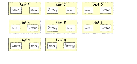
- Note that each level of the Treatment (Strong and Week) are applied to each Leaf (Block)
- Note that Treatments are randomly applied
- The Treatment effect is the mean difference between Treatment pairs per leaf
- Blocking in this way is very useful when spatial or temporal heterogeneity is likely to add noise that could make it difficualt to detect a difference between Treatments. Hence it is a way of experimentally reducing unexplained variation (compared to nesting which involves statistical reduction of unexplained variation).
Exploratory data analysis has indicated that the response variable could be normalized via a forth-root transformation.
- Fit the JAGS model for the Randomized Complete Block
- Effects parameterization - random intercepts model
number of lesionsi = βSite j(i) + εi where ε ∼ N(0,σ2)
View full code> runif(1)
[1] 0.7823
> modelString="
model {
   #Likelihood
   for (i in 1:n) {
      number[i]~dnorm(mean[i],tau.res)
      mean[i] <- beta.leaf[leaf[i]]+beta.treatment[treatment[i]]
      y.err[i] <- number[i] - mean[1]
   }

   #Priors and derivatives
   #alpha ~ dnorm(0,1.0E-6)
   #beta.leaf[1] <- 0
   for (i in 1:nLeaf) {
     beta.leaf[i] ~ dnorm(0,1.0E-6)
   }
   beta.treatment[1] <- 0
   for (i in 2:nTreat) {
     beta.treatment[i] ~ dnorm(0,1.0E-6)
   }

   Treatment.means[1] <- beta.leaf[1]+beta.treatment[1]
   Treatment.means[2] <- beta.leaf[1]+beta.treatment[2]

   tau.res <- pow(sigma.res,2)
   #sigma.res ~ dgamma(0.001,0.001)
   sigma.res ~ dunif(0,100)

   sd.Leaf <- sd(beta.leaf)
   sd.Treatment <- sd(beta.treatment)
   sd.Resid <- sd(y.err)

   perc.Treat <- 100*beta.treatment[2]/(Treatment.means[1]+1.0E-10)

   p.decline <- 1-step(beta.treatment[2])
   p.decline5 <- 1-step(beta.treatment[2]+Treatment.means[1]*0.05)
   p.decline10 <- 1-step(beta.treatment[2]+Treatment.means[1]*0.1)
   p.decline20 <- 1-step(beta.treatment[2]+Treatment.means[1]*0.2)
   p.decline50 <- 1-step(beta.treatment[2]+Treatment.means[1]*0.5)
   p.decline100 <- 1-step(beta.treatment[2]+Treatment.means[1]*1)
 }
"
> ## write the model to a text file (I suggest you alter the path to somewhere more relevant
> ## to your system!)
> writeLines(modelString,con="../downloads/BUGSscripts/ws9.8bQ1.1a.txt")
> tobacco.list <- with(tobacco,
+                          list(number=NUMBER,
+                             treatment=as.numeric(TREATMENT),
+                 leaf=as.numeric(LEAF),
+                             n=nrow(tobacco), nTreat=length(levels(as.factor(TREATMENT))),
+                                  nLeaf=length(levels(as.factor(LEAF)))
+                         )
+            )
> params <- c("perc.Treat","p.decline","p.decline5","p.decline10","p.decline20","p.decline50","p.decline100","Treatment.means","beta.leaf","beta.treatment","sigma.res","sd.Resid","sd.Leaf","sd.Treatment")
> adaptSteps = 1000
> burnInSteps = 200
> nChains = 3
> numSavedSteps = 5000
> thinSteps = 10
> nIter = ceiling((numSavedSteps * thinSteps)/nChains)
>
> library(R2jags)
> ##
> tobacco.r2jags <- jags(data=tobacco.list,
+           inits=NULL,#inits=list(inits,inits,inits), # since there are three chains
+           parameters.to.save=params,
+           model.file="../downloads/BUGSscripts/ws9.8bQ1.1a.txt",
+           n.chains=3,
+           n.iter=nIter,
+           n.burnin=burnInSteps,
+       n.thin=thinSteps
+           )
Compiling model graph
   Resolving undeclared variables
   Allocating nodes
   Graph Size: 136

Initializing model
> print(tobacco.r2jags)
Inference for Bugs model at "../downloads/BUGSscripts/ws9.8bQ1.1a.txt", fit using jags,
 3 chains, each with 16667 iterations (first 200 discarded), n.thin = 10
 n.sims = 4941 iterations saved
                   mu.vect sd.vect    2.5%     25%     50%     75%   97.5%  Rhat n.eff
Treatment.means[1]  34.379   3.164  27.938  32.499  34.377  36.352  40.616 1.002  2000
Treatment.means[2]  26.487   3.181  20.064  24.520  26.475  28.379  32.827 1.001  4000
beta.leaf[1]        34.379   3.164  27.938  32.499  34.377  36.352  40.616 1.002  2000
beta.leaf[2]        32.623   3.095  26.524  30.717  32.587  34.552  38.757 1.001  4900
beta.leaf[3]        33.857   3.116  27.603  31.929  33.815  35.730  40.144 1.001  4900
beta.leaf[4]        31.068   3.107  24.612  29.226  31.111  32.969  37.351 1.001  4900
beta.leaf[5]        32.997   3.038  26.917  31.137  32.963  34.943  39.039 1.001  4900
beta.leaf[6]        40.299   3.061  34.320  38.404  40.275  42.178  46.359 1.001  2900
beta.leaf[7]        43.514   3.080  37.218  41.663  43.517  45.461  49.468 1.001  4900
beta.leaf[8]        30.853   3.126  24.595  28.938  30.819  32.776  37.179 1.001  4900
beta.treatment[1]    0.000   0.000   0.000   0.000   0.000   0.000   0.000 1.000     1
beta.treatment[2]   -7.893   2.084 -12.000  -9.158  -7.929  -6.646  -3.635 1.001  4900
p.decline            0.999   0.032   1.000   1.000   1.000   1.000   1.000 1.189  1900
p.decline10          0.980   0.139   1.000   1.000   1.000   1.000   1.000 1.005  4900
p.decline100         0.000   0.000   0.000   0.000   0.000   0.000   0.000 1.000     1
p.decline20          0.722   0.448   0.000   0.000   1.000   1.000   1.000 1.002  2300
p.decline5           0.995   0.071   1.000   1.000   1.000   1.000   1.000 1.033  2900
p.decline50          0.000   0.014   0.000   0.000   0.000   0.000   0.000 1.291  4900
perc.Treat         -22.974   5.812 -34.315 -26.492 -23.019 -19.543 -11.027 1.001  4900
sd.Leaf              4.950   1.021   3.169   4.261   4.882   5.541   7.192 1.001  4900
sd.Resid             6.333   0.000   6.333   6.333   6.333   6.333   6.333 1.000     1
sd.Treatment         3.948   1.034   1.829   3.323   3.964   4.579   6.000 1.007  3900
sigma.res            0.272   0.069   0.147   0.223   0.268   0.318   0.414 1.001  4900
deviance            89.239   6.593  79.379  84.361  88.234  93.076 104.436 1.001  4900

For each parameter, n.eff is a crude measure of effective sample size,
and Rhat is the potential scale reduction factor (at convergence, Rhat=1).

DIC info (using the rule, pD = var(deviance)/2)
pD = 21.7 and DIC = 111.0
DIC is an estimate of expected predictive error (lower deviance is better).
Note that the Leaf β are not actually the leaf means. Rather they are the intercepts for each leaf (since we have fit a random intercepts model). They represent the value of the first Treatment level (Strong) within each Leaf.
The Treatment effect thus represents the mean of the differences between the second Treatment level (Week) and these intercepts.
Indeed, the analysis assumes that there is no real interactions between the Leafs (Blocks) and the Treatment effects (within Blocks) - otherwise the mean Treatment effect would be a over simplification of the true nature of the populations. The presence of such an interaction would indicate that the Blocks (Leafs) do not all represent the same population.
If we really want to explore whether there are Block by within block effects or obtain Leaf means that reflected the means of both levels of the Treatment, we can fit the full multiplicative model (random intercept and slope) and explore the marginal effects and interactions.View full code> runif(1)
[1] 0.8945
> modelString="
model {
   #Likelihood
   for (i in 1:n) {
      number[i]~dnorm(mean[i],tau.res)
      mean[i] <- beta[leaf[i],treatment[i]]
      y.err[i] <- number[i] - mean[1]
   }

   #Priors and derivatives
   for (i in 1:nLeaf) {
     for (j in 1:nTreat) {
       beta[i,j] ~ dnorm(0,1.0E-6)
     }
   }

   #Effects
   beta0 <- beta[1,1]
   for (i in 1:nLeaf) {
     beta.leaf[i] <- mean(beta[i,]-beta[1,])
   }
   #Leaf.means[1] <- mean(beta[1,])
   for (i in 1:nLeaf) {
     Leaf.means[i] <- mean(beta[i,])
   }
   for (i in 1:nTreat) {
     beta.treatment[i] <- mean(beta[,i]-beta[,1])
   }
   for (i in 1:nTreat) {
     Treatment.means[i] <- mean(beta[,i])
   }
   for (i in 1:nLeaf){
     for (j in 1:nTreat){
	   beta.int[i,j] <- beta[i,j]-beta.leaf[i]-beta.treatment[j]-beta0
	 }
   }


   tau.res <- pow(sigma.res,2)
   #sigma.res ~ dgamma(0.001,0.001)
   sigma.res ~ dunif(0,100)

   sd.Leaf <- sd(Leaf.means)
   sd.Treatment <- sd(Treatment.means)
   sd.Int <- sd(beta.int[,])
   sd.Resid <- sd(y.err)
 }
"
> ## write the model to a text file (I suggest you alter the path to somewhere more relevant
> ## to your system!)
> writeLines(modelString,con="../downloads/BUGSscripts/ws9.8bQ1.1b.txt")
> tobacco.list <- with(tobacco,
+                          list(number=NUMBER,
+                             treatment=as.numeric(TREATMENT),
+                 leaf=as.numeric(LEAF),
+                             n=nrow(tobacco), nTreat=length(levels(as.factor(TREATMENT))),
+                                  nLeaf=length(levels(as.factor(LEAF)))
+                         )
+            )
> params <- c("Leaf.means","Treatment.means","beta","beta.leaf","beta.treatment","sigma.res","sd.Leaf","sd.Treatment","sd.Int","sd.Resid")
> adaptSteps = 1000
> burnInSteps = 200
> nChains = 3
> numSavedSteps = 5000
> thinSteps = 10
> nIter = ceiling((numSavedSteps * thinSteps)/nChains)
>
> library(R2jags)
> ##
> tobacco.r2jags2 <- jags(data=tobacco.list,
+           inits=NULL,#inits=list(inits,inits,inits), # since there are three chains
+           parameters.to.save=params,
+           model.file="../downloads/BUGSscripts/ws9.8bQ1.1b.txt",
+           n.chains=3,
+           n.iter=nIter,
+           n.burnin=burnInSteps,
+       n.thin=thinSteps
+           )
Compiling model graph
   Resolving undeclared variables
   Allocating nodes
   Graph Size: 185

Initializing model
> print(tobacco.r2jags2)
Inference for Bugs model at "../downloads/BUGSscripts/ws9.8bQ1.1b.txt", fit using jags,
 3 chains, each with 16667 iterations (first 200 discarded), n.thin = 10
 n.sims = 4941 iterations saved
                   mu.vect sd.vect     2.5%     25%     50%     75%  97.5%  Rhat n.eff
Leaf.means[1]       30.456   1.841   30.362  30.449  30.459  30.469 30.568 1.289  4900
Leaf.means[2]       28.659   1.462   28.524  28.633  28.643  28.653 28.741 1.288  4900
Leaf.means[3]       29.880   2.837   29.809  29.902  29.912  29.922 30.007 1.290  4900
Leaf.means[4]       27.125   2.627   26.970  27.072  27.082  27.092 27.198 1.288  4900
Leaf.means[5]       29.097   2.137   28.996  29.093  29.103  29.112 29.206 1.288  4900
Leaf.means[6]       36.331   3.032   36.257  36.351  36.361  36.370 36.470 1.290  4900
Leaf.means[7]       39.578   1.313   39.498  39.594  39.604  39.614 39.696 1.286  3600
Leaf.means[8]       26.810   2.170   26.743  26.830  26.841  26.851 26.951 1.290  4600
Treatment.means[1]  34.916   1.487   34.888  34.935  34.940  34.945 34.993 1.291  4000
Treatment.means[2]  27.068   0.651   27.007  27.056  27.061  27.066 27.109 1.289  4900
beta[1,1]           35.871   1.870   35.754  35.884  35.898  35.912 36.054 1.289  3800
beta[2,1]           34.147   2.085   33.954  34.103  34.118  34.132 34.249 1.289  4500
beta[3,1]           35.638   3.459   35.551  35.688  35.702  35.717 35.843 1.290  3400
beta[4,1]           26.217   2.066   26.072  26.210  26.225  26.239 26.390 1.289  4900
beta[5,1]           33.011   4.340   32.871  33.003  33.017  33.030 33.156 1.290  4900
beta[6,1]           36.675   5.364   36.588  36.714  36.729  36.743 36.906 1.290  4900
beta[7,1]           44.708   1.798   44.549  44.709  44.724  44.737 44.859 1.288  4900
beta[8,1]           33.063   2.284   32.959  33.095  33.110  33.124 33.255 1.290  2300
beta[1,2]           25.040   2.420   24.880  25.006  25.020  25.034 25.154 1.289  4900
beta[2,2]           23.171   1.631   23.017  23.153  23.167  23.182 23.313 1.287  4900
beta[3,2]           24.121   2.872   23.971  24.108  24.122  24.136 24.252 1.290  4900
beta[4,2]           28.033   4.857   27.778  27.925  27.939  27.953 28.082 1.289  4900
beta[5,2]           25.183   1.865   25.039  25.175  25.189  25.203 25.324 1.285  4900
beta[6,2]           35.987   1.457   35.842  35.979  35.993  36.007 36.152 1.288  4900
beta[7,2]           34.449   2.620   34.332  34.470  34.485  34.499 34.624 1.287  4900
beta[8,2]           20.557   3.206   20.438  20.557  20.572  20.586 20.712 1.290  4900
beta.leaf[1]         0.000   0.000    0.000   0.000   0.000   0.000  0.000 1.000     1
beta.leaf[2]        -1.797   2.811   -1.969  -1.831  -1.817  -1.803 -1.696 1.290  4900
beta.leaf[3]        -0.576   3.385   -0.707  -0.561  -0.547  -0.533 -0.402 1.290  4900
beta.leaf[4]        -3.331   3.589   -3.530  -3.392  -3.377  -3.364 -3.218 1.290  4900
beta.leaf[5]        -1.358   1.818   -1.489  -1.370  -1.357  -1.342 -1.215 1.288  4900
beta.leaf[6]         5.876   3.090    5.756   5.888   5.901   5.915  6.058 1.290  4900
beta.leaf[7]         9.123   1.483    9.004   9.130   9.145   9.158  9.277 1.283  4900
beta.leaf[8]        -3.646   2.182   -3.771  -3.633  -3.618  -3.604 -3.473 1.290  4900
beta.treatment[1]    0.000   0.000    0.000   0.000   0.000   0.000  0.000 1.000     1
beta.treatment[2]   -7.849   1.438   -7.962  -7.886  -7.879  -7.872 -7.810 1.291  2300
sd.Int               2.599   1.726    2.485   2.512   2.516   2.519  2.563 1.290   240
sd.Leaf              4.345   1.886    4.243   4.269   4.273   4.277  4.320 1.294   290
sd.Resid             6.333   0.000    6.333   6.333   6.333   6.333  6.333 1.000     1
sd.Treatment         3.954   0.531    3.908   3.936   3.940   3.943  3.982 1.285  2300
sigma.res           51.752  28.688    2.331  27.783  52.065  76.524 97.783 1.052   140
deviance           -71.200  33.611 -105.396 -93.245 -80.673 -60.124 17.555 1.051   140

For each parameter, n.eff is a crude measure of effective sample size,
and Rhat is the potential scale reduction factor (at convergence, Rhat=1).

DIC info (using the rule, pD = var(deviance)/2)
pD = 556.9 and DIC = 485.7
DIC is an estimate of expected predictive error (lower deviance is better).
View full code> runif(1)
[1] 0.34
> modelString="
model {
   #Likelihood
   for (i in 1:n) {
      number[i]~dnorm(mean[i],tau.res)
	  mean[i] <- alpha+beta.leaf[leaf[i]] + beta.treatment[treatment[i]] + beta.int[leaf[i],treatment[i]]
      y.err[i] <- number[i] - mean[1]
   }

   #Priors and derivatives


  alpha ~ dnorm(0,1.0E-6)
  beta.leaf[1] <- 0
  beta.int[1,1] <- 0
  for (i in 2:nLeaf) {
     beta.leaf[i] ~ dnorm(0,1.0E-6)
     beta.int[i,1] <-0
  }
  beta.treatment[1] <- 0
  for (i in 2:nTreat) {
    beta.treatment[i] ~ dnorm(0,1.0E-6)
	beta.int[1,i] <- 0
  }

  for (i in 2:nLeaf) {
    for (j in 2:nTreat) {
	  beta.int[i,j] ~ dnorm(0,1.0E-6)
	}
  }
   tau.res <- pow(sigma.res,2)
   #sigma.res ~ dgamma(0.001,0.001)
   sigma.res ~ dunif(0,100)

 }
"
> ## write the model to a text file (I suggest you alter the path to somewhere more relevant
> ## to your system!)
> writeLines(modelString,con="../downloads/BUGSscripts/ws9.8bQ1.1c.txt")
> tobacco.list <- with(tobacco,
+                          list(number=NUMBER,
+                             treatment=as.numeric(TREATMENT),
+                 leaf=as.numeric(LEAF),
+                             n=nrow(tobacco), nTreat=length(levels(as.factor(TREATMENT))),
+                                  nLeaf=length(levels(as.factor(LEAF)))
+                         )
+            )
> params <- c("alpha","beta.leaf","beta.treatment","beta.int","sigma.res")
> adaptSteps = 1000
> burnInSteps = 200
> nChains = 3
> numSavedSteps = 5000
> thinSteps = 10
> nIter = ceiling((numSavedSteps * thinSteps)/nChains)
>
> library(R2jags)
> ##
> tobacco.r2jags3 <- jags(data=tobacco.list,
+           inits=NULL,#inits=list(inits,inits,inits), # since there are three chains
+           parameters.to.save=params,
+           model.file="../downloads/BUGSscripts/ws9.8bQ1.1c.txt",
+           n.chains=3,
+           n.iter=nIter,
+           n.burnin=burnInSteps,
+       n.thin=thinSteps
+           )
Compiling model graph
   Resolving undeclared variables
   Allocating nodes
   Graph Size: 116

Initializing model
> print(tobacco.r2jags3)
Inference for Bugs model at "../downloads/BUGSscripts/ws9.8bQ1.1c.txt", fit using jags,
 3 chains, each with 16667 iterations (first 200 discarded), n.thin = 10
 n.sims = 4941 iterations saved
                  mu.vect sd.vect     2.5%     25%     50%     75%   97.5%  Rhat n.eff
alpha              35.878   1.255   35.734  35.883  35.897  35.911  36.048 1.234  1500
beta.int[1,1]       0.000   0.000    0.000   0.000   0.000   0.000   0.000 1.000     1
beta.int[2,1]       0.000   0.000    0.000   0.000   0.000   0.000   0.000 1.000     1
beta.int[3,1]       0.000   0.000    0.000   0.000   0.000   0.000   0.000 1.000     1
beta.int[4,1]       0.000   0.000    0.000   0.000   0.000   0.000   0.000 1.000     1
beta.int[5,1]       0.000   0.000    0.000   0.000   0.000   0.000   0.000 1.000     1
beta.int[6,1]       0.000   0.000    0.000   0.000   0.000   0.000   0.000 1.000     1
beta.int[7,1]       0.000   0.000    0.000   0.000   0.000   0.000   0.000 1.000     1
beta.int[8,1]       0.000   0.000    0.000   0.000   0.000   0.000   0.000 1.000     1
beta.int[1,2]       0.000   0.000    0.000   0.000   0.000   0.000   0.000 1.000     1
beta.int[2,2]      -0.070   2.953   -0.431  -0.101  -0.073  -0.046   0.216 1.253  4900
beta.int[3,2]      -0.657   2.908   -1.003  -0.732  -0.702  -0.675  -0.377 1.244  4900
beta.int[4,2]      12.574   2.514   12.226  12.564  12.592  12.619  12.859 1.219  4900
beta.int[5,2]       3.059   2.935    2.727   3.021   3.049   3.077   3.390 1.206  4900
beta.int[6,2]      10.083   3.013    9.831  10.112  10.142  10.170  10.445 1.209  2200
beta.int[7,2]       0.622   2.382    0.298   0.610   0.637   0.664   0.930 1.253  4900
beta.int[8,2]      -1.697   2.309   -1.963  -1.689  -1.661  -1.634  -1.367 1.224  4900
beta.leaf[1]        0.000   0.000    0.000   0.000   0.000   0.000   0.000 1.000     1
beta.leaf[2]       -1.740   2.310   -2.005  -1.800  -1.780  -1.760  -1.537 1.254  1900
beta.leaf[3]       -0.209   1.542   -0.425  -0.215  -0.195  -0.176  -0.003 1.186  4900
beta.leaf[4]       -9.652   2.362   -9.871  -9.692  -9.673  -9.653  -9.429 1.232  4900
beta.leaf[5]       -2.863   2.258   -3.080  -2.900  -2.881  -2.861  -2.643 1.240  3800
beta.leaf[6]        0.888   2.008    0.627   0.811   0.831   0.851   1.051 1.251   940
beta.leaf[7]        8.854   1.940    8.618   8.806   8.826   8.846   9.082 1.225  4200
beta.leaf[8]       -2.761   1.544   -2.982  -2.807  -2.788  -2.768  -2.555 1.234  3500
beta.treatment[1]   0.000   0.000    0.000   0.000   0.000   0.000   0.000 1.000     1
beta.treatment[2] -10.882   1.871  -11.074 -10.896 -10.877 -10.857 -10.633 1.241  4900
sigma.res          52.309  29.008    2.121  27.030  54.293  77.575  97.780 1.021   220
deviance          -71.311  34.429 -105.821 -93.649 -81.370 -59.776  21.548 1.021   210

For each parameter, n.eff is a crude measure of effective sample size,
and Rhat is the potential scale reduction factor (at convergence, Rhat=1).

DIC info (using the rule, pD = var(deviance)/2)
pD = 587.3 and DIC = 516.0
DIC is an estimate of expected predictive error (lower deviance is better).
In the above, alpha is the mean (value) of the Strong Treatment in Leaf 1. βTreatment 2 is the difference between the value of the Strong and Week Treatments in Leaf 1.
- Effects parameterization - random intercepts model
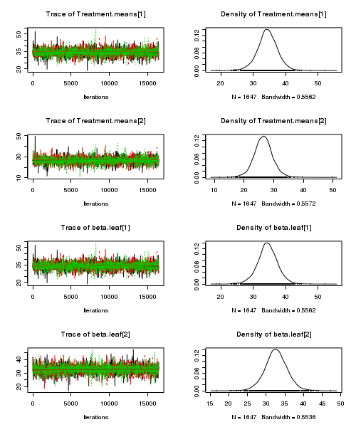
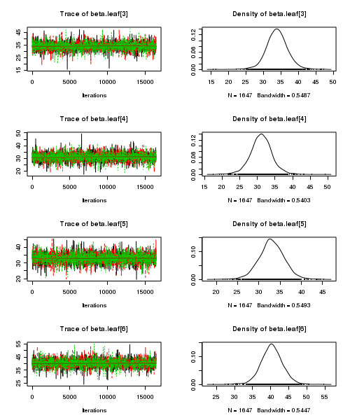
- Before fully exploring the parameters, it is prudent to examine the convergence and mixing diagnostics.
Chose either the effects or means parameterization model (they should yield much the same).
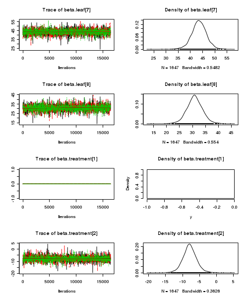
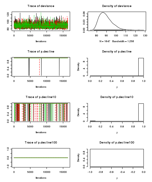
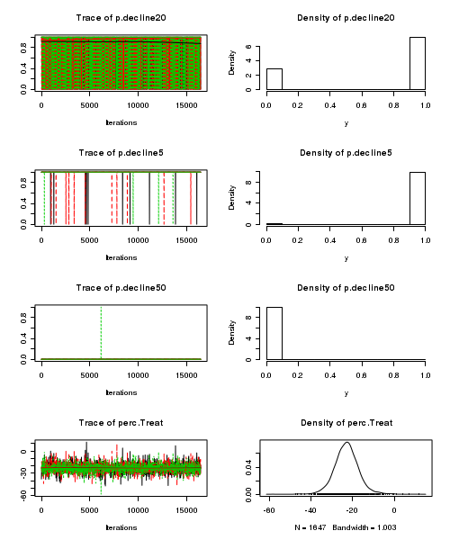
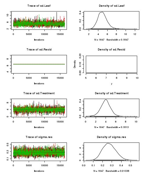
- Trace plots
View code
> plot(as.mcmc(tobacco.r2jags))
- Raftery diagnostic
View code
> raftery.diag(as.mcmc(tobacco.r2jags))
[[1]]

Quantile (q) = 0.025
Accuracy (r) = +/- 0.005
Probability (s) = 0.95

You need a sample size of at least 3746 with these values of q, r and s

[[2]]

Quantile (q) = 0.025
Accuracy (r) = +/- 0.005
Probability (s) = 0.95

You need a sample size of at least 3746 with these values of q, r and s

[[3]]

Quantile (q) = 0.025
Accuracy (r) = +/- 0.005
Probability (s) = 0.95

You need a sample size of at least 3746 with these values of q, r and s
- Autocorrelation
View code
> autocorr.diag(as.mcmc(tobacco.r2jags))
        Treatment.means[1] Treatment.means[2] beta.leaf[1] beta.leaf[2] beta.leaf[3] beta.leaf[4]
Lag 0            1.0000000           1.000000    1.0000000     1.000000     1.000000      1.00000
Lag 10           0.0008802           0.006387    0.0008802     0.009082     0.010568     -0.02105
Lag 50           0.0163591           0.020910    0.0163591    -0.021316     0.006175      0.01663
Lag 100          0.0103684           0.014494    0.0103684     0.012102     0.004241     -0.01814
Lag 500         -0.0039647           0.006587   -0.0039647     0.006971     0.013273     -0.02884
        beta.leaf[5] beta.leaf[6] beta.leaf[7] beta.leaf[8] beta.treatment[1] beta.treatment[2]
Lag 0       1.000000      1.00000    1.0000000     1.000000               NaN         1.0000000
Lag 10      0.002638     -0.01812    0.0241051     0.017104               NaN         0.0047574
Lag 50      0.012203     -0.01305   -0.0051696    -0.003514               NaN        -0.0114785
Lag 100     0.027296     -0.01367   -0.0222627    -0.011227               NaN        -0.0003129
Lag 500    -0.009941      0.01217    0.0003319     0.020987               NaN        -0.0041822
         deviance p.decline p.decline10 p.decline100 p.decline20 p.decline5 p.decline50 perc.Treat
Lag 0    1.000000       NaN   1.0000000          NaN    1.000000   1.000000         NaN   1.000000
Lag 10   0.009082       NaN  -0.0008481          NaN    0.006289  -0.005092         NaN   0.006519
Lag 50   0.020272       NaN   0.0088339          NaN    0.014328  -0.005104         NaN  -0.005918
Lag 100 -0.015875       NaN  -0.0201543          NaN    0.008923  -0.005120         NaN   0.004018
Lag 500 -0.015573       NaN   0.0006197          NaN    0.017398  -0.004837         NaN   0.003894
          sd.Leaf sd.Resid sd.Treatment sigma.res
Lag 0    1.000000      NaN    1.000e+00  1.000000
Lag 10   0.005889      NaN    6.826e-03  0.036491
Lag 50   0.002473      NaN   -1.070e-02  0.003780
Lag 100 -0.008857      NaN   -5.059e-05  0.002928
Lag 500  0.025602      NaN   -3.433e-03  0.012135
- Trace plots
-
A summary figure would be nice
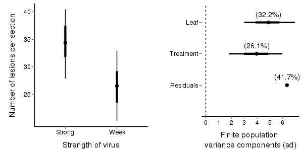
View code
> tobacco.mcmc <- as.mcmc(tobacco.r2jags$BUGSoutput$sims.matrix)
> #get the column indexes for the parameters we are interested in
> tobacco.sum <- summary.mcmc(tobacco.mcmc, terms=c("^Treatment"))
> tobacco.sum$Treatment <- c("Strong","Week")
>
>                                                  p1<-ggplot(tobacco.sum,aes(y=mean, x=Treatment))+
+ geom_errorbar(aes(ymin=lower, ymax=upper),width=0,size=1.5,position=position_dodge(0.2))+
+ geom_errorbar(aes(ymin=lower.1, ymax=upper.1),width=0,position=position_dodge(0.2))+
+ geom_point(size=3)+
+ scale_y_continuous("Number of lesions per section")+
+ scale_x_discrete("Strength of virus")+
+ murray_opts
>
>
> #Finite-population standard deviations
> tobacco.sd <- summary.mcmc(tobacco.mcmc, terms=c("sd"))
> rownames(tobacco.sd) <- c("Leaf", "Residuals", "Treatment")
> tobacco.sd$name <- factor(c("Leaf", "Residuals", "Treatment"), levels=c("Residuals", "Treatment","Leaf"))
>
> p2<-ggplot(tobacco.sd,aes(y=name, x=median))+
+ geom_vline(xintercept=0,linetype="dashed")+
+ geom_hline(xintercept=0)+
+ scale_x_continuous("Finite population \nvariance components (sd)")+
+ geom_errorbarh(aes(xmin=lower.1, xmax=upper.1), height=0, size=1)+
+ geom_errorbarh(aes(xmin=lower, xmax=upper), height=0, size=1.5)+
+ geom_point(size=3)+
+ geom_text(aes(label=sprintf("(%4.1f%%)",Perc),vjust=-1))+
+ murray_opts+
+ opts(axis.line=theme_blank(),axis.title.y=theme_blank(),
+ axis.text.y=theme_text(size=12,hjust=1))
>
> grid.newpage()
> pushViewport(viewport(layout=grid.layout(1,2,5,5,respect=TRUE)))
> pushViewport(viewport(layout.pos.col=1, layout.pos.row=1))
> print(p1,newpage=FALSE)
> popViewport(1)
> pushViewport(viewport(layout.pos.col=2, layout.pos.row=1))
> print(p2,newpage=FALSE)
> popViewport(0)