Workshop 9.9b - Mixed effects (multilevel models): Split-plot and Complex Randomized block designs (Bayesian)
23 April 2011
Split-plot ANOVA (Mixed effects) references
- McCarthy (2007) - Chpt ?
- Kery (2010) - Chpt ?
- Gelman & Hill (2007) - Chpt ?
- Logan (2010) - Chpt 13
- Quinn & Keough (2002) - Chpt 10
> library(R2jags)
> library(ggplot2)
> library(grid)
> #define my common ggplot options
> murray_opts <- opts(panel.grid.major=theme_blank(),
+ 			   panel.grid.minor=theme_blank(),
+ 			   panel.border = theme_blank(),
+ 			   panel.background = theme_blank(),
+ 			   axis.title.y=theme_text(size=15, vjust=0,angle=90),
+ 			   axis.text.y=theme_text(size=12),
+ 			   axis.title.x=theme_text(size=15, vjust=-1),
+ 			   axis.text.x=theme_text(size=12),
+ 			   axis.line = theme_segment(),
+ 			   legend.position=c(1,0.1),legend.justification=c(1,0),
+ 			   legend.key=theme_blank(),
+ 			   plot.margin=unit(c(0.5,0.5,1,2),"lines")
+ )
>
> #create a convenience function for predicting from mcmc objects
> predict.mcmc <- function(mcmc, terms=NULL, mmat, trans="identity") {
+   library(plyr)
+   library(coda)
+   if(is.null(terms)) mcmc.coefs <- mcmc
+   else 	{
+      iCol<-match(terms, colnames(mcmc))
+ 	 mcmc.coefs <- mcmc[,iCol]
+   }
+   t2=")"
+   if (trans=="identity") {
+ 	t1 <- ""
+ 	t2=""
+   }else if (trans=="log") {
+ 	t1="exp("
+   }else if (trans=="log10") {
+ 	t1="10^("
+   }else if (trans=="sqrt") {
+ 	t1="("
+ 	t2=")^2"
+   }
+   eval(parse(text=paste("mcmc.sum <-adply(mcmc.coefs %*% t(mmat),2,function(x) {
+ 	data.frame(mean=",t1,"mean(x)",t2,",
+     median=",t1,"median(x)",t2,",
+ 	",t1,"coda:::HPDinterval(as.mcmc(x), p=0.68)",t2,",
+ 	",t1,"coda:::HPDinterval(as.mcmc(x))",t2,"
+     )})", sep="")))
+
+   mcmc.sum
+ }
>
>
> #create a convenience function for summarizing mcmc objects
> summary.mcmc <- function(mcmc, terms=NULL, trans="identity") {
+   library(plyr)
+   library(coda)
+   if(is.null(terms)) mcmc.coefs <- mcmc
+   else 	{
+      iCol<-grep(terms, colnames(mcmc))
+ 	 mcmc.coefs <- mcmc[,iCol]
+   }
+   t2=")"
+   if (trans=="identity") {
+ 	t1 <- ""
+ 	t2=""
+   }else if (trans=="log") {
+ 	t1="exp("
+   }else if (trans=="log10") {
+ 	t1="10^("
+   }else if (trans=="sqrt") {
+ 	t1="("
+ 	t2=")^2"
+   }
+   eval(parse(text=paste("mcmc.sum <-adply(mcmc.coefs,2,function(x) {
+ 	data.frame(mean=",t1,"mean(x)",t2,",
+     median=",t1,"median(x)",t2,",
+ 	",t1,"coda:::HPDinterval(as.mcmc(x), p=0.68)",t2,",
+ 	",t1,"coda:::HPDinterval(as.mcmc(x))",t2,"
+     )})", sep="")))
+
+   mcmc.sum$Perc <-100*mcmc.sum$median/sum(mcmc.sum$median)
+   mcmc.sum
+ }
Split-plot
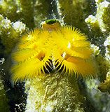
Split-plotIn an attempt to understand the effects on marine animals of short-term exposure to toxic substances, such as might occur following a spill, or a major increase in storm water flows, a it was decided to examine the toxicant in question, Copper, as part of a field experiment in Honk Kong. The experiment consisted of small sources of Cu (small, hemispherical plaster blocks, impregnated with copper), which released the metal into sea water over 4 or 5 days. The organism whose response to Cu was being measured was a small, polychaete worm, Hydroides, that attaches to hard surfaces in the sea, and is one of the first species to colonize any surface that is submerged. The biological questions focused on whether the timing of exposure to Cu affects the overall abundance of these worms. The time period of interest was the first or second week after a surface being available.
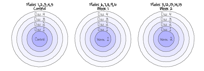
The experimental setup consisted of sheets of black perspex (settlement plates), which provided good surfaces for these worms. Each plate had a plaster block bolted to its centre, and the dissolving block would create a gradient of [Cu] across the plate. Over the two weeks of the experiment, a given plate would have pl ain plaster blocks (Control) or a block containing copper in the first week, followed by a plain block, or a plain block in the first week, followed by a dose of copper in the second week. After two weeks in the water, plates were removed and counted back in the laboratory. Without a clear idea of how sensitive these worms are to copper, an effect of the treatments might show up as an overall difference in the density of worms across a plate, or it could show up as a gradient in abundance across the plate, with a different gradient in different treatments. Therefore, on each plate, the density of worms (#/cm2) was recorded at each of four distances from the center of the plate.
Download Copper data set| Format of copper.csv data file | |||||||||||||||||
|---|---|---|---|---|---|---|---|---|---|---|---|---|---|---|---|---|---|
|
 |
> copper <- read.table("../downloads/data/copper.csv",
+     header = T, sep = ",", strip.white = T)
> head(copper)
   COPPER PLATE DIST WORMS
1 control   200    4 11.50
2 control   200    3 13.00
3 control   200    2 13.50
4 control   200    1 12.00
5 control    39    4 17.75
6 control    39    3 13.75
The Plates are the "random" groups. Within each Plate, all levels of the Distance factor occur (this is a within group factor). Each Plate can only be of one of the three levels of the Copper treatment. This is therefore a within group (nested) factor. Traditionally, this mixture of nested and randomized block design would be called a partly nested or split-plot design.
In Bayesian (multilevel modeling) terms, this is a multi-level model with one hierarchical level the Plates means and another representing the Copper treatment means (based on the Plate means).
Exploratory data analysis has indicated that the response variable could be normalized via a forth-root transformation.
- Fit the JAGS model for the Randomized Complete Block
- Effects parameterization - random intercepts model
number of lesionsi = βSite j(i) + εi where ε ∼ N(0,σ2)treating Distance as a factor
View full code> > runif(1)[1] 0.5445
> modelString="
+ model {
+    #Likelihood
+    for (i in 1:n) {
+       worms[i]~dnorm(mean[i],tau.res)
+       mean[i] <- beta.plate[plate[i]]+beta.dist[dist[i]]+beta.CopperDist[cu[i],dist[i]]
+       y.err[i] <- worms[i] - mean[1]
+    }
+
+    #Priors and derivatives
+    for (j in 1:nPlate) {
+       beta.plate[j] ~ dnorm(mu.plate[j],tau.plate)
+       mu.plate[j] <- g0+gamma.copper[copper[j]]
+ 	  y.plate.err[j] <- beta.plate[j] - mu.plate[j]
+    }
+    g0 ~ dnorm(0.0,1.0E-6)
+    gamma.copper[1] <- 0
+    for (i in 2:nCopper) {
+      gamma.copper[i] ~ dnorm(mu.copper, tau.copper)
+    }
+    mu.copper ~ dnorm(0,1.0E-6)
+
+    beta.dist[1] <- 0
+    for (j in 2:nDist) {
+      beta.dist[j] ~ dnorm(mu.dist,tau.dist)
+    }
+    mu.dist ~ dnorm(0,1.0E-6)
+
+    beta.CopperDist[1,1] <- 0
+    for (i in 2:nCopper) {
+      beta.CopperDist[i,1] <- 0
+    }
+    for (j in 2:nDist) {
+      beta.CopperDist[1,j] <- 0
+    }
+    for (i in 2:nCopper) {
+      for (j in 2:nDist) {
+ 	    beta.CopperDist[i,j] ~ dnorm(mu.copperdist,tau.copperdist)
+ 	 }
+    }
+    mu.copperdist ~ dnorm(0,1.0E-6)
+
+    sigma.res ~ dunif(0,100) #prior on sd residuals
+    tau.res <- 1 / (sigma.res * sigma.res)
+    sigma.plate ~ dunif(0, 100) #prior on sd residuals
+    tau.plate <- 1 / (sigma.plate * sigma.plate)
+
+    sigma.copper ~ dunif(0, 100) #prior on sd residuals
+    tau.copper <- 1 / (sigma.copper * sigma.copper)
+    sigma.dist ~ dunif(0, 100) #prior on sd residuals
+    tau.dist <- 1 / (sigma.dist * sigma.dist)
+    sigma.copperdist ~ dunif(0, 100) #prior on sd residuals
+    tau.copperdist <- 1 / (sigma.copperdist * sigma.copperdist)
+
+    sd.Resid <- sd(y.err)
+    sd.Plate <- sd(y.plate.err)
+    sd.Copper <- sd(gamma.copper)
+    sd.Dist <- sd(beta.dist)
+    sd.CopperDist <- sd(beta.CopperDist)
+
+    #Generate means
+    for (i in 1:nCopper) {
+      Copper.means[i] <- g0+gamma.copper[i]
+    }
+    for (i in 1:nDist) {
+      Dist.means[i] <- mean(beta.plate[])+beta.dist[i]
+    }
+    for (i in 1:nCopper) {
+      for (j in 1:nDist) {
+ 	    CopperDist.means[i,j] <- g0 + gamma.copper[i] + beta.dist[j]+ beta.CopperDist[i,j]
+ 	 }
+    }
+  }
+ "
> ## write the model to a text file (I suggest you alter the path to somewhere more relevant
> ## to your system!)
> writeLines(modelString,con="../downloads/BUGSscripts/ws9.9bQ2.1a.txt")
>
>
> #sort the data set so that the copper treatments are in a more logical order
> copper.sort <- copper[order(copper$COPPER),]
> copper.sort$COPPER <- factor(copper.sort$COPPER, levels = c("control", "Week 1", "Week 2"))
> copper.sort$PLATE <- factor(copper.sort$PLATE, levels=unique(copper.sort$PLATE))
> cu <- with(copper.sort,COPPER[match(unique(PLATE),PLATE)])
> cu <- factor(cu, levels=c("control", "Week 1", "Week 2"))
> copper.list <- with(copper.sort,
+ 			 list(worms=WORMS,
+ 			   dist=as.numeric(DIST),
+                plate=as.numeric(PLATE),
+ 			   copper=factor(as.numeric(cu)),
+                cu=as.numeric(COPPER),
+ 			   nDist=length(levels(as.factor(DIST))),
+ 			   nPlate=length(levels(as.factor(PLATE))),
+ 			   nCopper=length(levels(cu)),
+ 			   n=nrow(copper.sort)
+ 			   )
+ 			   )
> params <- c("g0","gamma.copper",
+ 		  "beta.plate",
+           "beta.dist",
+ 		  "beta.CopperDist",
+ 		  "Copper.means","Dist.means","CopperDist.means",
+ 		  "sd.Dist","sd.Copper","sd.Plate","sd.Resid","sd.CopperDist",
+ 		  "sigma.res","sigma.plate","sigma.copper","sigma.dist","sigma.copperdist"
+ 		  )
> adaptSteps = 1000
> burnInSteps = 2000
> nChains = 3
> numSavedSteps = 5000
> thinSteps = 10
> nIter = ceiling((numSavedSteps * thinSteps)/nChains)
>
> library(R2jags)
> ##
> copper.r2jags <- jags(data=copper.list,
+ 				 inits=NULL, # since there are three chains
+ 	  parameters.to.save=params,
+ 	  model.file="../downloads/BUGSscripts/ws9.9bQ2.1a.txt",
+ 	  n.chains=3,
+ 	  n.iter=nIter,
+ 	  n.burnin=burnInSteps,
+       n.thin=thinSteps
+ 	  )
Compiling model graph Resolving undeclared variables Allocating nodes Graph Size: 458 Initializing model
> print(copper.r2jags)Inference for Bugs model at "../downloads/BUGSscripts/ws9.9bQ2.1a.txt", fit using jags, 3 chains, each with 16667 iterations (first 2000 discarded), n.thin = 10 n.sims = 4401 iterations saved mu.vect sd.vect 2.5% 25% 50% 75% 97.5% Rhat n.eff Copper.means[1] 10.827 0.679 9.480 10.367 10.820 11.285 12.149 1.002 1900 Copper.means[2] 6.975 0.673 5.696 6.523 6.961 7.414 8.319 1.001 4400 Copper.means[3] 0.480 0.683 -0.826 0.028 0.477 0.931 1.824 1.003 770 CopperDist.means[1,1] 10.827 0.679 9.480 10.367 10.820 11.285 12.149 1.002 1900 CopperDist.means[2,1] 6.975 0.673 5.696 6.523 6.961 7.414 8.319 1.001 4400 CopperDist.means[3,1] 0.480 0.683 -0.826 0.028 0.477 0.931 1.824 1.003 770 CopperDist.means[1,2] 12.016 0.679 10.699 11.565 12.022 12.477 13.378 1.001 2700 CopperDist.means[2,2] 8.419 0.687 7.054 7.977 8.414 8.859 9.806 1.001 2800 CopperDist.means[3,2] 1.571 0.689 0.235 1.113 1.563 2.026 2.969 1.001 4400 CopperDist.means[1,3] 12.441 0.634 11.186 12.018 12.447 12.871 13.674 1.001 4400 CopperDist.means[2,3] 8.593 0.693 7.257 8.140 8.604 9.042 9.960 1.001 4400 CopperDist.means[3,3] 3.958 0.690 2.592 3.501 3.966 4.428 5.316 1.001 4400 CopperDist.means[1,4] 13.512 0.697 12.144 13.038 13.515 13.971 14.885 1.002 1900 CopperDist.means[2,4] 10.083 0.670 8.783 9.638 10.074 10.531 11.393 1.001 4400 CopperDist.means[3,4] 7.558 0.710 6.142 7.100 7.573 8.035 8.929 1.001 4400 Dist.means[1] 6.091 0.362 5.379 5.854 6.094 6.333 6.784 1.002 1700 Dist.means[2] 7.280 0.773 5.763 6.770 7.289 7.810 8.764 1.002 1900 Dist.means[3] 7.704 0.741 6.261 7.200 7.709 8.196 9.118 1.002 2400 Dist.means[4] 8.776 0.793 7.240 8.253 8.762 9.295 10.342 1.002 1700 beta.CopperDist[1,1] 0.000 0.000 0.000 0.000 0.000 0.000 0.000 1.000 1 beta.CopperDist[2,1] 0.000 0.000 0.000 0.000 0.000 0.000 0.000 1.000 1 beta.CopperDist[3,1] 0.000 0.000 0.000 0.000 0.000 0.000 0.000 1.000 1 beta.CopperDist[1,2] 0.000 0.000 0.000 0.000 0.000 0.000 0.000 1.000 1 beta.CopperDist[2,2] 0.255 1.204 -2.077 -0.554 0.227 1.070 2.672 1.001 2700 beta.CopperDist[3,2] -0.098 1.181 -2.414 -0.888 -0.079 0.685 2.185 1.002 1600 beta.CopperDist[1,3] 0.000 0.000 0.000 0.000 0.000 0.000 0.000 1.000 1 beta.CopperDist[2,3] 0.005 1.175 -2.292 -0.782 -0.005 0.803 2.363 1.002 2300 beta.CopperDist[3,3] 1.865 1.166 -0.397 1.075 1.871 2.648 4.171 1.001 2800 beta.CopperDist[1,4] 0.000 0.000 0.000 0.000 0.000 0.000 0.000 1.000 1 beta.CopperDist[2,4] 0.423 1.163 -1.877 -0.344 0.389 1.164 2.770 1.003 930 beta.CopperDist[3,4] 4.393 1.282 1.785 3.554 4.420 5.240 6.824 1.001 4400 beta.dist[1] 0.000 0.000 0.000 0.000 0.000 0.000 0.000 1.000 1 beta.dist[2] 1.189 0.851 -0.521 0.614 1.199 1.776 2.831 1.002 1800 beta.dist[3] 1.614 0.825 -0.015 1.065 1.622 2.168 3.211 1.002 1300 beta.dist[4] 2.685 0.867 1.017 2.108 2.670 3.252 4.413 1.003 920 beta.plate[1] 6.866 0.695 5.531 6.409 6.864 7.332 8.237 1.002 2400 beta.plate[2] 6.522 0.750 4.972 6.036 6.549 7.016 7.936 1.001 4400 beta.plate[3] 7.255 0.732 5.889 6.751 7.250 7.743 8.728 1.001 4400 beta.plate[4] 7.099 0.718 5.725 6.623 7.082 7.576 8.532 1.001 4400 beta.plate[5] 7.124 0.721 5.732 6.648 7.114 7.604 8.557 1.002 4300 beta.plate[6] 0.405 0.721 -0.972 -0.085 0.399 0.880 1.846 1.003 880 beta.plate[7] 0.335 0.730 -1.096 -0.158 0.343 0.815 1.753 1.002 1200 beta.plate[8] 0.340 0.727 -1.044 -0.139 0.340 0.825 1.752 1.003 1000 beta.plate[9] 0.681 0.735 -0.721 0.190 0.676 1.173 2.139 1.004 630 beta.plate[10] 0.615 0.724 -0.753 0.122 0.608 1.087 2.060 1.002 2300 beta.plate[11] 10.942 0.726 9.532 10.450 10.933 11.430 12.364 1.002 1300 beta.plate[12] 11.560 0.870 9.940 10.952 11.534 12.141 13.334 1.001 4400 beta.plate[13] 10.431 0.765 8.937 9.925 10.434 10.933 11.927 1.001 3700 beta.plate[14] 10.484 0.739 9.036 9.999 10.497 10.972 11.919 1.002 1900 beta.plate[15] 10.704 0.734 9.240 10.222 10.705 11.197 12.169 1.001 3000 g0 10.827 0.679 9.480 10.367 10.820 11.285 12.149 1.002 1900 gamma.copper[1] 0.000 0.000 0.000 0.000 0.000 0.000 0.000 1.000 1 gamma.copper[2] -3.852 0.954 -5.777 -4.483 -3.843 -3.215 -1.991 1.002 1900 gamma.copper[3] -10.347 0.950 -12.194 -10.977 -10.346 -9.753 -8.435 1.002 2000 sd.Copper 4.288 0.388 3.489 4.039 4.285 4.538 5.054 1.002 1400 sd.CopperDist 1.420 0.328 0.782 1.206 1.413 1.633 2.072 1.001 4400 sd.Dist 1.048 0.300 0.473 0.846 1.041 1.248 1.662 1.003 1100 sd.Plate 0.502 0.260 0.047 0.311 0.502 0.680 1.018 1.004 4300 sd.Resid 4.268 0.000 4.268 4.268 4.268 4.268 4.268 1.000 1 sigma.copper 30.726 26.101 2.849 9.150 21.619 46.811 92.783 1.001 4400 sigma.copperdist 2.642 1.499 0.926 1.704 2.279 3.121 6.628 1.001 4400 sigma.dist 3.705 6.332 0.140 0.857 1.656 3.595 22.586 1.003 3000 sigma.plate 0.572 0.331 0.051 0.328 0.548 0.768 1.305 1.004 2800 sigma.res 1.405 0.167 1.125 1.287 1.391 1.504 1.764 1.001 4400 deviance 209.167 8.422 193.466 203.287 209.216 214.763 225.686 1.001 4400 For each parameter, n.eff is a crude measure of effective sample size, and Rhat is the potential scale reduction factor (at convergence, Rhat=1). DIC info (using the rule, pD = var(deviance)/2) pD = 35.5 and DIC = 244.6 DIC is an estimate of expected predictive error (lower deviance is better).
- Effects parameterization - random intercepts model
-
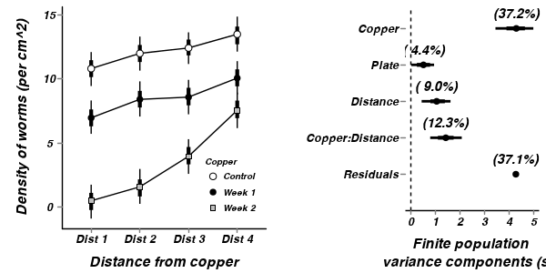
A summary figure would be nice
View code
> copper.mcmc <- as.mcmc(copper.r2jags$BUGSoutput$sims.matrix)
> #get the column indexes for the parameters we are interested in
> copper.sum <- summary.mcmc(copper.mcmc, terms=c("CopperDist.means"))
> copper.sum <- cbind(copper.sum, expand.grid(Copper=c("Control","Week 1","Week 2"), Distance=paste("Dist ",1:4,sep="")))
>
> p1<-ggplot(copper.sum,aes(y=mean, x=Distance, group=Copper))+
+ geom_line()+
+ geom_errorbar(aes(ymin=lower, ymax=upper),width=0,size=1.5)+
+ geom_errorbar(aes(ymin=lower.1, ymax=upper.1),width=0)+
+ geom_point(aes(shape=Copper, fill=Copper),size=3)+
+ scale_y_continuous("Density of worms (per cm^2)")+
+ scale_x_discrete("Distance from copper")+
+ scale_shape_manual(name="Copper",values=c(21,16,22), breaks=c("Control","Week 1","Week 2"), labels=c("Control","Week 1","Week 2"))+
+ scale_fill_manual(name="Copper",values=c("white","black","grey"), breaks=c("Control","Week 1","Week 2"), labels=c("Control","Week 1","Week 2"))+
+ murray_opts+opts(legend.position=c(1,0),legend.justification=c(1,0))
>
>
> #Finite-population standard deviations
> copper.sd <- summary.mcmc(copper.mcmc, terms=c("sd"))
> rownames(copper.sd) <- c("Copper","Copper:Distance","Distance", "Plate","Residuals")
> copper.sd$name <- factor(rownames(copper.sd), levels=c("Residuals","Copper:Distance","Distance", "Plate","Copper"))
>
> p2<-ggplot(copper.sd,aes(y=name, x=median))+
+ geom_vline(xintercept=0,linetype="dashed")+
+ geom_hline(xintercept=0)+
+ scale_x_continuous("Finite population \nvariance components (sd)")+
+ geom_errorbarh(aes(xmin=lower.1, xmax=upper.1), height=0, size=1)+
+ geom_errorbarh(aes(xmin=lower, xmax=upper), height=0, size=1.5)+
+ geom_point(size=3)+
+ geom_text(aes(label=sprintf("(%4.1f%%)",Perc),vjust=-1))+
+ murray_opts+
+ opts(axis.line=theme_blank(),axis.title.y=theme_blank(),
+ axis.text.y=theme_text(size=12,hjust=1))
>
> grid.newpage()
> pushViewport(viewport(layout=grid.layout(1,2,5,5,respect=TRUE)))
> pushViewport(viewport(layout.pos.col=1, layout.pos.row=1))
> print(p1,newpage=FALSE)
> popViewport(1)
> pushViewport(viewport(layout.pos.col=2, layout.pos.row=1))
> print(p2,newpage=FALSE)
> popViewport(0)
>
>
> #eff and eff2
> #copper.eff <- summary.mcmc(copper.mcmc, terms=c("eff"))
> #rows <- c(matrix(upper.tri(diag(paste("S",1:4,sep=""))),ncol=1)[,1],rep(TRUE,4))
> #nms <- paste("Situation",1:4)
> #nms <- with(expand.grid(S1=nms, S2=nms),paste(S1,S2,sep=" vs "))
> #nms <- c(nms,"Nov - Jan (S1)","Nov - Jan (S2)","Nov - Jan (S3)","Nov - Jan (S4)")
> #copper.eff$name <- nms
> #copper.eff <- copper.eff[rows,]
>
> #p3 <- ggplot(copper.eff, aes(y=name, x=mean))+
> #geom_vline(xintercept=0,linetype="dashed")+
> #geom_hline(xintercept=0)+
> #geom_errorbarh(aes(xmin=lower.1, xmax=upper.1), height=0, size=1)+
> #geom_errorbarh(aes(xmin=lower, xmax=upper), height=0, size=1.5)+
> #geom_point(size=3)+murray_opts+
> #scale_x_continuous(name="Effect size")+
> #opts(axis.line=theme_blank(),axis.title.y=theme_blank(),
> #axis.text.y=theme_text(size=12,hjust=1))
> #p3
>
>
>
> ##cohen's D
> #eff<-NULL
> #eff.sd <- NULL
> #for (i in seq(1,7,b=2)) {
> #  eff <-cbind(eff,copper.mcmc[,i] - copper.mcmc[,i+1])
> #  eff.sd <- cbind(eff.sd,mean(apply(copper.mcmc[,i:(i+1)],2,sd)))
> #}
> #cohen <- sweep(eff,2,eff.sd,"/")
> #adply(cohen,2,function(x) {
> #   data.frame(mean=mean(x), median=median(x),
> #		 HPDinterval(as.mcmc(x), p=0.68), HPDinterval(as.mcmc(x)))
> #})
Repeated Measures
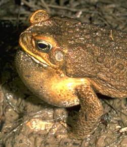
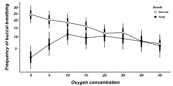
Repeated MeasuresIn an honours thesis from (1992), Mullens was investigating the ways that cane toads ( Bufo marinus ) respond to conditions of hypoxia. Toads show two different kinds of breathing patterns, lung or buccal, requiring them to be treated separately in the experiment. Her aim was to expose toads to a range of O2 concentrations, and record their breathing patterns, including parameters such as the expired volume for individual breaths. It was desirable to have around 8 replicates to compare the responses of the two breathing types, and the complication is that animals are expensive, and different individuals are likely to have different O2 profiles (leading to possibly reduced power). There are two main design options for this experiment;
- One animal per O2 treatment, 8 concentrations, 2 breathing types. With 8 replicates the experiment would require 128 animals, but that this could be analysed as a completely randomized design
- One O2 profile per animal, so that each animal would be used 8 times and only 16 animals are required (8 lung and 8 buccal breathers)
| Format of mullens.csv data file | |||||||||||||||||||||||||||||||||||||||||
|---|---|---|---|---|---|---|---|---|---|---|---|---|---|---|---|---|---|---|---|---|---|---|---|---|---|---|---|---|---|---|---|---|---|---|---|---|---|---|---|---|---|
|
 |
> mullens <- read.table("../downloads/data/mullens.csv", header = T,
+     sep = ",", strip.white = T)
> head(mullens)
  BREATH TOAD O2LEVEL FREQBUC SFREQBUC
1   lung    a       0    10.6    3.256
2   lung    a       5    18.8    4.336
3   lung    a      10    17.4    4.171
4   lung    a      15    16.6    4.074
5   lung    a      20     9.4    3.066
6   lung    a      30    11.4    3.376
Notice that the BREATH variable contains a categorical listing of the breathing type and that the first entries begin with "l" with comes after "b" in the alphabet (and therefore when BREATH is converted into a numeric, the first entry will be a 2. So we need to be careful that our codes reflect the order of the data.
Exploratory data analysis indicated that a square-root transformation of the FREQBUC (response variable) could normalize this variable and thereby address heterogeneity issues. Consequently, we too will apply a square-root transformation.
- Fit the JAGS model for the Randomized Complete Block
- Effects parameterization - random intercepts model
number of lesionsi = βSite j(i) + εi where ε ∼ N(0,σ2)
View full code> runif(1)[1] 0.2225
> modelString="
+ data {
+   sfreqbuc <- sqrt(freqbuc)
+ }
+ model {
+    #Likelihood
+    for (i in 1:n) {
+       sfreqbuc[i]~dnorm(mean[i],tau.res)
+       mean[i] <- beta.toad[toad[i]]+beta.o2level[cO2level[i]]+beta.BreathO2level[breath[i],cO2level[i]]
+ 	  #mean[i] <- beta.toad[toad[i]] +beta.o2level[cO2level[i]] #+beta.BreathO2level[br[i],o2level[i]]
+       y.err[i] <- sfreqbuc[i] - mean[1]
+    }
+
+    #Priors and derivatives
+    for (j in 1:nToad) {
+       beta.toad[j] ~ dnorm(mu.toad[j],tau.toad)
+       #mu.toad[j] ~ dnorm(0,1.0E-6)
+       mu.toad[j] <- g0+gamma.breath[br[j]]
+ 	  y.toad.err[j] <- beta.toad[j] - mu.toad[j]
+    }
+    g0 ~ dnorm(0.0,1.0E-6)
+    gamma.breath[1] <- 0
+    for (i in 2:nBreath) {
+      gamma.breath[i] ~ dnorm(mu.breath, tau.breath)
+    }
+    mu.breath ~ dnorm(0,1.0E-6)
+
+    beta.o2level[1] <- 0
+    for (j in 2:nO2level) {
+      beta.o2level[j] ~ dnorm(mu.o2level,tau.o2level)
+    }
+    mu.o2level ~ dnorm(0,1.0E-6)
+
+    beta.BreathO2level[1,1] <- 0
+    for (i in 2:nBreath) {
+      beta.BreathO2level[i,1] <- 0
+    }
+    for (j in 2:nO2level) {
+      beta.BreathO2level[1,j] <- 0
+    }
+    for (i in 2:nBreath) {
+      for (j in 2:nO2level) {
+ 	    beta.BreathO2level[i,j] ~ dnorm(mu.breatho2level,tau.breatho2level)
+ 	 }
+    }
+    mu.breatho2level ~ dnorm(0,1.0E-6)
+
+    sigma.res ~ dunif(0,100) #prior on sd residuals
+    tau.res <- 1 / (sigma.res * sigma.res)
+    sigma.toad ~ dunif(0, 100) #prior on sd residuals
+    tau.toad <- 1 / (sigma.toad * sigma.toad)
+
+    sigma.breath ~ dunif(0, 100) #prior on sd residuals
+    tau.breath <- 1 / (sigma.breath * sigma.breath)
+    sigma.o2level ~ dunif(0, 100) #prior on sd residuals
+    tau.o2level <- 1 / (sigma.o2level * sigma.o2level)
+    sigma.breatho2level ~ dunif(0, 100) #prior on sd residuals
+    tau.breatho2level <- 1 / (sigma.breatho2level * sigma.breatho2level)
+
+    sd.Resid <- sd(y.err)
+    sd.Toad <- sd(y.toad.err)
+    sd.Breath <- sd(gamma.breath)
+    sd.O2level <- sd(beta.o2level)
+    sd.BreathO2level <- sd(beta.BreathO2level)
+
+    #Generate means
+    for (i in 1:nBreath) {
+      Breath.means[i] <- g0+gamma.breath[i]
+    }
+    for (i in 1:nO2level) {
+      O2level.means[i] <- mean(beta.toad[])+beta.o2level[i]
+    }
+    for (i in 1:nBreath) {
+      for (j in 1:nO2level) {
+  	    BreathO2level.means[i,j] <- g0 + gamma.breath[i] + beta.o2level[j]+ beta.BreathO2level[i,j]
+ 	 }
+    }
+  }
+ "
> ## write the model to a text file (I suggest you alter the path to somewhere more relevant
> ## to your system!)
> writeLines(modelString,con="../downloads/BUGSscripts/ws9.9bQ3.1a.txt")
>
>
> #sort the data set so that the breath treatments are in a more logical order
> mullens.sort <- mullens[order(mullens$BREATH),]
> mullens.sort$BREATH <- factor(mullens.sort$BREATH, levels = c("buccal", "lung"))
> mullens.sort$TOAD <- factor(mullens.sort$TOAD, levels=unique(mullens.sort$TOAD))
> br <- with(mullens.sort,BREATH[match(unique(TOAD),TOAD)])
> br <- factor(br, levels=c("buccal", "lung"))
> mullens.list <- with(mullens.sort,
+ 			 list(freqbuc=FREQBUC,
+ 			   o2level=as.numeric(O2LEVEL),
+                cO2level=as.numeric(as.factor(O2LEVEL)),
+                toad=as.numeric(TOAD),
+ 			   br=factor(as.numeric(br)),
+                breath=as.numeric(BREATH),
+ 			   nO2level=length(levels(as.factor(O2LEVEL))),
+ 			   nToad=length(levels(as.factor(TOAD))),
+ 			   nBreath=length(levels(br)),
+ 			   n=nrow(mullens.sort)
+ 			   )
+ 			   )
> params <- c(
+ 		  "g0","gamma.breath",
+ 		  "beta.toad",
+           "beta.o2level",
+ 		  "beta.BreathO2level",
+ 		  "Breath.means","O2level.means","BreathO2level.means",
+ 		  "sd.O2level","sd.Breath","sd.Toad","sd.Resid","sd.BreathO2level",
+ 		  "sigma.res","sigma.toad","sigma.breath","sigma.o2level","sigma.breatho2level"
+ 		  )
> adaptSteps = 1000
> burnInSteps = 2000
> nChains = 3
> numSavedSteps = 5000
> thinSteps = 10
> nIter = ceiling((numSavedSteps * thinSteps)/nChains)
>
> library(R2jags)
> ##
> mullens.r2jags <- jags(data=mullens.list,
+ 				 inits=NULL, # since there are three chains
+ 	  parameters.to.save=params,
+ 	  model.file="../downloads/BUGSscripts/ws9.9bQ3.1a.txt",
+ 	  n.chains=3,
+ 	  n.iter=nIter,
+ 	  n.burnin=burnInSteps,
+       n.thin=thinSteps
+ 	  )
Compiling data graph Resolving undeclared variables Allocating nodes Initializing Reading data back into data table Compiling model graph Resolving undeclared variables Allocating nodes Graph Size: 1252 Initializing model
> print(mullens.r2jags)Inference for Bugs model at "../downloads/BUGSscripts/ws9.9bQ3.1a.txt", fit using jags, 3 chains, each with 16667 iterations (first 2000 discarded), n.thin = 10 n.sims = 4401 iterations saved mu.vect sd.vect 2.5% 25% 50% 75% 97.5% Rhat n.eff Breath.means[1] 4.927 0.364 4.224 4.693 4.924 5.164 5.642 1.002 2000 Breath.means[2] 1.543 0.470 0.637 1.221 1.552 1.853 2.460 1.001 4400 BreathO2level.means[1,1] 4.927 0.364 4.224 4.693 4.924 5.164 5.642 1.002 2000 BreathO2level.means[2,1] 1.543 0.470 0.637 1.221 1.552 1.853 2.460 1.001 4400 BreathO2level.means[1,2] 4.513 0.361 3.799 4.268 4.511 4.753 5.221 1.001 4400 BreathO2level.means[2,2] 2.556 0.477 1.620 2.236 2.547 2.867 3.531 1.001 2400 BreathO2level.means[1,3] 4.293 0.356 3.598 4.057 4.294 4.529 4.990 1.001 4400 BreathO2level.means[2,3] 3.367 0.453 2.489 3.069 3.368 3.672 4.257 1.001 4000 BreathO2level.means[1,4] 4.007 0.349 3.326 3.780 4.000 4.236 4.699 1.002 1900 BreathO2level.means[2,4] 3.086 0.461 2.159 2.774 3.089 3.393 3.976 1.001 3100 BreathO2level.means[1,5] 3.450 0.348 2.769 3.215 3.445 3.680 4.144 1.001 4400 BreathO2level.means[2,5] 3.231 0.450 2.348 2.933 3.237 3.533 4.118 1.002 2000 BreathO2level.means[1,6] 3.502 0.348 2.808 3.280 3.501 3.733 4.185 1.001 4400 BreathO2level.means[2,6] 3.028 0.458 2.116 2.732 3.026 3.327 3.931 1.001 2500 BreathO2level.means[1,7] 2.829 0.358 2.112 2.596 2.829 3.065 3.534 1.001 4400 BreathO2level.means[2,7] 2.818 0.451 1.945 2.518 2.820 3.122 3.704 1.001 4400 BreathO2level.means[1,8] 2.623 0.360 1.925 2.384 2.621 2.861 3.337 1.001 2400 BreathO2level.means[2,8] 2.474 0.458 1.529 2.188 2.488 2.766 3.380 1.001 3300 O2level.means[1] 3.641 0.194 3.256 3.512 3.639 3.773 4.030 1.001 2800 O2level.means[2] 3.227 0.290 2.657 3.033 3.228 3.425 3.790 1.001 4400 O2level.means[3] 3.007 0.279 2.463 2.818 3.010 3.194 3.573 1.001 4400 O2level.means[4] 2.721 0.271 2.191 2.535 2.718 2.904 3.261 1.001 4400 O2level.means[5] 2.164 0.271 1.634 1.982 2.162 2.342 2.698 1.001 4400 O2level.means[6] 2.216 0.271 1.689 2.036 2.214 2.397 2.749 1.001 4400 O2level.means[7] 1.543 0.279 1.002 1.355 1.544 1.727 2.098 1.001 4400 O2level.means[8] 1.337 0.286 0.784 1.145 1.335 1.537 1.898 1.001 4400 beta.BreathO2level[1,1] 0.000 0.000 0.000 0.000 0.000 0.000 0.000 1.000 1 beta.BreathO2level[2,1] 0.000 0.000 0.000 0.000 0.000 0.000 0.000 1.000 1 beta.BreathO2level[1,2] 0.000 0.000 0.000 0.000 0.000 0.000 0.000 1.000 1 beta.BreathO2level[2,2] 1.427 0.584 0.298 1.035 1.424 1.824 2.575 1.001 4400 beta.BreathO2level[1,3] 0.000 0.000 0.000 0.000 0.000 0.000 0.000 1.000 1 beta.BreathO2level[2,3] 2.458 0.534 1.422 2.095 2.458 2.821 3.490 1.001 4400 beta.BreathO2level[1,4] 0.000 0.000 0.000 0.000 0.000 0.000 0.000 1.000 1 beta.BreathO2level[2,4] 2.463 0.532 1.419 2.093 2.462 2.816 3.518 1.001 4400 beta.BreathO2level[1,5] 0.000 0.000 0.000 0.000 0.000 0.000 0.000 1.000 1 beta.BreathO2level[2,5] 3.165 0.536 2.110 2.804 3.160 3.529 4.219 1.001 4400 beta.BreathO2level[1,6] 0.000 0.000 0.000 0.000 0.000 0.000 0.000 1.000 1 beta.BreathO2level[2,6] 2.910 0.531 1.888 2.549 2.901 3.278 3.953 1.001 4400 beta.BreathO2level[1,7] 0.000 0.000 0.000 0.000 0.000 0.000 0.000 1.000 1 beta.BreathO2level[2,7] 3.373 0.548 2.288 2.994 3.377 3.754 4.429 1.001 4400 beta.BreathO2level[1,8] 0.000 0.000 0.000 0.000 0.000 0.000 0.000 1.000 1 beta.BreathO2level[2,8] 3.235 0.545 2.144 2.874 3.231 3.606 4.280 1.001 4400 beta.o2level[1] 0.000 0.000 0.000 0.000 0.000 0.000 0.000 1.000 1 beta.o2level[2] -0.414 0.353 -1.115 -0.652 -0.414 -0.173 0.285 1.001 3000 beta.o2level[3] -0.634 0.343 -1.305 -0.866 -0.630 -0.401 0.032 1.001 4400 beta.o2level[4] -0.921 0.334 -1.581 -1.143 -0.921 -0.695 -0.271 1.001 4400 beta.o2level[5] -1.477 0.333 -2.136 -1.701 -1.476 -1.262 -0.824 1.001 3700 beta.o2level[6] -1.425 0.337 -2.094 -1.653 -1.427 -1.196 -0.759 1.001 3800 beta.o2level[7] -2.098 0.342 -2.753 -2.326 -2.099 -1.870 -1.435 1.001 2800 beta.o2level[8] -2.304 0.347 -2.979 -2.544 -2.304 -2.070 -1.627 1.001 4400 beta.toad[1] 4.287 0.373 3.565 4.033 4.287 4.547 5.006 1.003 1000 beta.toad[2] 6.297 0.379 5.551 6.042 6.296 6.556 7.019 1.002 1300 beta.toad[3] 4.693 0.378 3.963 4.433 4.687 4.949 5.436 1.001 4400 beta.toad[4] 4.380 0.376 3.654 4.119 4.377 4.635 5.119 1.002 2300 beta.toad[5] 6.356 0.382 5.622 6.094 6.353 6.618 7.103 1.001 2800 beta.toad[6] 4.131 0.376 3.378 3.877 4.129 4.381 4.858 1.001 3600 beta.toad[7] 3.688 0.377 2.958 3.434 3.678 3.944 4.429 1.001 2800 beta.toad[8] 4.448 0.375 3.696 4.205 4.449 4.697 5.156 1.001 4400 beta.toad[9] 5.947 0.374 5.204 5.698 5.948 6.200 6.673 1.001 4400 beta.toad[10] 4.832 0.367 4.115 4.585 4.830 5.075 5.553 1.001 4400 beta.toad[11] 4.962 0.380 4.207 4.710 4.961 5.213 5.700 1.001 4400 beta.toad[12] 5.613 0.372 4.881 5.358 5.618 5.862 6.334 1.002 1200 beta.toad[13] 4.457 0.373 3.730 4.208 4.455 4.709 5.201 1.001 4400 beta.toad[14] 1.985 0.418 1.145 1.706 1.989 2.268 2.803 1.001 4400 beta.toad[15] 2.824 0.420 1.975 2.544 2.824 3.104 3.657 1.001 4400 beta.toad[16] 1.289 0.415 0.484 1.011 1.291 1.563 2.103 1.001 4400 beta.toad[17] 0.969 0.414 0.158 0.698 0.973 1.249 1.779 1.001 4400 beta.toad[18] 0.284 0.421 -0.541 0.001 0.282 0.564 1.121 1.001 4400 beta.toad[19] 2.182 0.419 1.351 1.903 2.186 2.463 3.016 1.002 1900 beta.toad[20] 1.588 0.417 0.768 1.302 1.592 1.872 2.409 1.001 4400 beta.toad[21] 1.258 0.415 0.438 0.980 1.255 1.537 2.075 1.001 4400 g0 4.927 0.364 4.224 4.693 4.924 5.164 5.642 1.002 2000 gamma.breath[1] 0.000 0.000 0.000 0.000 0.000 0.000 0.000 1.000 1 gamma.breath[2] -3.384 0.597 -4.579 -3.778 -3.381 -2.986 -2.193 1.002 2100 sd.Breath 1.692 0.298 1.097 1.493 1.691 1.889 2.289 1.001 2400 sd.BreathO2level 1.430 0.201 1.041 1.292 1.429 1.566 1.811 1.001 4400 sd.O2level 0.784 0.091 0.597 0.725 0.786 0.846 0.961 1.001 4400 sd.Resid 1.478 0.000 1.478 1.478 1.478 1.478 1.478 1.000 1 sd.Toad 0.862 0.082 0.710 0.809 0.859 0.911 1.033 1.001 2800 sigma.breath 50.668 28.857 2.479 25.979 51.336 75.338 97.788 1.001 4400 sigma.breatho2level 0.969 0.474 0.365 0.658 0.870 1.155 2.077 1.001 4400 sigma.o2level 0.964 0.431 0.460 0.686 0.871 1.128 2.043 1.001 4400 sigma.res 0.880 0.056 0.779 0.840 0.877 0.916 1.000 1.001 2900 sigma.toad 0.944 0.185 0.654 0.812 0.922 1.048 1.376 1.001 4400 deviance 432.461 10.265 414.450 425.277 431.669 438.804 454.986 1.001 2900 For each parameter, n.eff is a crude measure of effective sample size, and Rhat is the potential scale reduction factor (at convergence, Rhat=1). DIC info (using the rule, pD = var(deviance)/2) pD = 52.7 and DIC = 485.1 DIC is an estimate of expected predictive error (lower deviance is better).
- Effects parameterization - random intercepts model
-
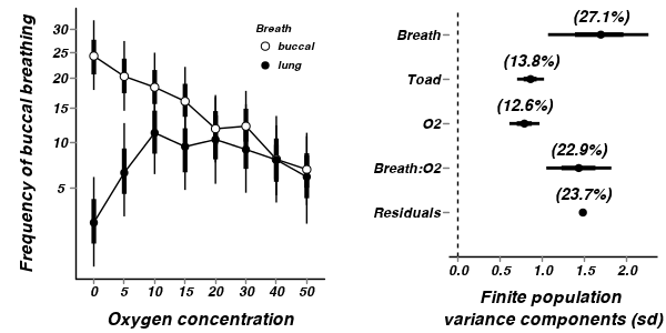
A summary figure would be nice
View code
> mullens.mcmc <- as.mcmc(mullens.r2jags$BUGSoutput$sims.matrix)
> #get the column indexes for the parameters we are interested in
> mullens.sum <- summary.mcmc(mullens.mcmc, terms=c("BreathO2level.means"))
> mullens.sum <- cbind(mullens.sum, expand.grid(Breath=c("buccal","lung"), O2level=paste("O2 ",c(0,5,10,15,20,30,40,50),sep="")))
> #
> library(scales)
> p1<-ggplot(mullens.sum,aes(y=mean, x=O2level, group=Breath))+
+ geom_line()+
+ geom_errorbar(aes(ymin=lower, ymax=upper),width=0,size=1.5)+
+ geom_errorbar(aes(ymin=lower.1, ymax=upper.1),width=0)+
+ geom_point(aes(shape=Breath, fill=Breath),size=3)+
+ scale_y_continuous("Frequency of buccal breathing",
+ 	#trans=trans_new("x2",function(x) {x^2},function(x) {sqrt(x);}),
+     breaks=trans_breaks(function(x) {print(x);x^2}, "sqrt"),
+     labels=trans_format(function(x) {x^2}, format=format_format()))+
+ scale_x_discrete("Oxygen concentration", breaks=paste("O2 ",c(0,5,10,15,20,30,40,50),sep=""), labels=c(0,5,10,15,20,30,40,50))+
+ scale_shape_manual(name="Breath",values=c(21,16), breaks=c("buccal","lung"), labels=c("buccal","lung"))+
+ scale_fill_manual(name="Breath",values=c("white","black"), breaks=c("buccal","lung"), labels=c("buccal","lung"))+
+ murray_opts+opts(legend.position=c(1,1),legend.justification=c(1,1))
> p1
[1] 0.3994 5.9033
>
> #Finite-population standard deviations
> mullens.sd <- summary.mcmc(mullens.mcmc, terms=c("sd"))
> rownames(mullens.sd) <- c("Breath","Breath:O2","O2", "Residuals","Toad")
> mullens.sd$name <- factor(rownames(mullens.sd), levels=c("Residuals","Breath:O2","O2", "Toad","Breath"))
>
> p2<-ggplot(mullens.sd,aes(y=name, x=median))+
+ geom_vline(xintercept=0,linetype="dashed")+
+ geom_hline(xintercept=0)+
+ scale_x_continuous("Finite population \nvariance components (sd)")+
+ geom_errorbarh(aes(xmin=lower.1, xmax=upper.1), height=0, size=1)+
+ geom_errorbarh(aes(xmin=lower, xmax=upper), height=0, size=1.5)+
+ geom_point(size=3)+
+ geom_text(aes(label=sprintf("(%4.1f%%)",Perc),vjust=-1))+
+ murray_opts+
+ opts(axis.line=theme_blank(),axis.title.y=theme_blank(),
+ axis.text.y=theme_text(size=12,hjust=1))
>
> grid.newpage()
> pushViewport(viewport(layout=grid.layout(1,2,5,5,respect=TRUE)))
> pushViewport(viewport(layout.pos.col=1, layout.pos.row=1))
> print(p1,newpage=FALSE)
[1] 0.3994 5.9033
> popViewport(1)
> pushViewport(viewport(layout.pos.col=2, layout.pos.row=1))
> print(p2,newpage=FALSE)
> popViewport(0)
- Fit the JAGS model for the Randomized Complete Block
- Effects parameterization - random intercepts model
number of lesionsi = βSite j(i) + εi where ε ∼ N(0,σ2)
View full code> runif(1)[1] 0.02771
> modelString="
+ data {
+   sfreqbuc <- sqrt(freqbuc)
+ }
+ model {
+    #Likelihood
+    for (i in 1:n) {
+       sfreqbuc[i]~dnorm(mean[i],tau.res)
+       mean[i] <- beta.toad[toad[i]]+beta.o2level*o2level[i]+
+                  beta.o2level2*o2level2[i]+
+                  beta.BreathO2level[breath[i]]*o2level[i]+
+                  beta.BreathO2level2[breath[i]]*o2level2[i]
+
+       y.err[i] <- sfreqbuc[i] - mean[1]
+    }
+
+    #Priors and derivatives
+    for (j in 1:nToad) {
+       beta.toad[j] ~ dnorm(mu.toad[j],tau.toad)
+       #mu.toad[j] ~ dnorm(0,1.0E-6)
+       mu.toad[j] <- g0+gamma.breath[br[j]]
+ 	  y.toad.err[j] <- beta.toad[j] - mu.toad[j]
+    }
+    g0 ~ dnorm(0.0,1.0E-6)
+    gamma.breath[1] <- 0
+    for (i in 2:nBreath) {
+      gamma.breath[i] ~ dnorm(mu.breath, tau.breath)
+    }
+    mu.breath ~ dnorm(0,1.0E-6)
+
+    beta.o2level ~ dnorm(mu.o2level,tau.o2level)
+    mu.o2level ~ dnorm(0,1.0E-6)
+    beta.o2level2 ~ dnorm(mu.o2level2,tau.o2level2)
+    mu.o2level2 ~ dnorm(0,1.0E-6)
+
+    beta.BreathO2level[1] <- 0
+    beta.BreathO2level2[1] <- 0
+    for (i in 2:nBreath) {
+      beta.BreathO2level[i] ~ dnorm(mu.breatho2level,tau.breatho2level)
+      beta.BreathO2level2[i] ~ dnorm(mu.breatho2level2,tau.breatho2level2)
+    }
+    mu.breatho2level ~ dnorm(0,1.0E-6)
+    mu.breatho2level2 ~ dnorm(0,1.0E-6)
+
+    sigma.res ~ dunif(0,100) #prior on sd residuals
+    tau.res <- 1 / (sigma.res * sigma.res)
+    sigma.toad ~ dunif(0, 100) #prior on sd residuals
+    tau.toad <- 1 / (sigma.toad * sigma.toad)
+
+    sigma.breath ~ dunif(0, 100) #prior on sd residuals
+    tau.breath <- 1 / (sigma.breath * sigma.breath)
+    sigma.o2level ~ dunif(0, 100) #prior on sd residuals
+    tau.o2level <- 1 / (sigma.o2level * sigma.o2level)
+    sigma.o2level2 ~ dunif(0, 100) #prior on sd residuals
+    tau.o2level2 <- 1 / (sigma.o2level2 * sigma.o2level2)
+    sigma.breatho2level ~ dunif(0, 100) #prior on sd residuals
+    tau.breatho2level <- 1 / (sigma.breatho2level * sigma.breatho2level)
+    sigma.breatho2level2 ~ dunif(0, 100) #prior on sd residuals
+    tau.breatho2level2 <- 1 / (sigma.breatho2level2 * sigma.breatho2level2)
+
+    sd.Resid <- sd(y.err)
+    sd.Toad <- sd(y.toad.err)
+    sd.Breath <- sd(gamma.breath)
+    sd.O2level <- abs(beta.o2level)*sd(o2level)
+    sd.BreathO2level <- sd(beta.BreathO2level)
+
+    #Generate means
+    for (i in 1:nBreath) {
+      Breath.means[i] <- g0+gamma.breath[i]
+    }
+
+
+  }
+ "
> ## write the model to a text file (I suggest you alter the path to somewhere more relevant
> ## to your system!)
> writeLines(modelString,con="../downloads/BUGSscripts/ws9.9bQ3.4a.txt")
>
>
> #sort the data set so that the breath treatments are in a more logical order
> mullens.sort <- mullens[order(mullens$BREATH),]
> mullens.sort$BREATH <- factor(mullens.sort$BREATH, levels = c("buccal", "lung"))
> mullens.sort$TOAD <- factor(mullens.sort$TOAD, levels=unique(mullens.sort$TOAD))
> br <- with(mullens.sort,BREATH[match(unique(TOAD),TOAD)])
> br <- factor(br, levels=c("buccal", "lung"))
> mullens.list2 <- with(mullens.sort,
+ 			 list(freqbuc=FREQBUC,
+ 			   o2level=as.numeric(scale(O2LEVEL,scale=FALSE)), #note this was a little lazy, we should center within each toad (but as the levels are identical within each toad, it will yield the same)
+ 				  o2level2=as.numeric(scale(O2LEVEL^2,scale=FALSE)),
+                toad=as.numeric(TOAD),
+ 			   br=factor(as.numeric(br)),
+                breath=as.numeric(BREATH),
+ 			   nToad=length(levels(as.factor(TOAD))),
+ 			   nBreath=length(levels(br)),
+ 			   n=nrow(mullens.sort)
+ 			   )
+ 			   )
> params <- c(
+ 		  "g0","gamma.breath",
+ 		  "beta.toad",
+           "beta.o2level",
+ 		  "beta.o2level2",
+ 		  "beta.BreathO2level",
+ 		  "beta.BreathO2level2",
+ 		  "Breath.means",
+ 		  "sd.O2level","sd.Breath","sd.Toad","sd.Resid","sd.BreathO2level",
+ 		  "sigma.res","sigma.toad","sigma.breath","sigma.o2level","sigma.breatho2level"
+ 		  )
> adaptSteps = 1000
> burnInSteps = 2000
> nChains = 3
> numSavedSteps = 5000
> thinSteps = 10
> nIter = ceiling((numSavedSteps * thinSteps)/nChains)
>
> library(R2jags)
> ##
> mullens.r2jags2 <- jags(data=mullens.list2,
+ 				 inits=NULL, # since there are three chains
+ 	  parameters.to.save=params,
+ 	  model.file="../downloads/BUGSscripts/ws9.9bQ3.4a.txt",
+ 	  n.chains=3,
+ 	  n.iter=nIter,
+ 	  n.burnin=burnInSteps,
+       n.thin=thinSteps
+ 	  )
Compiling data graph Resolving undeclared variables Allocating nodes Initializing Reading data back into data table Compiling model graph Resolving undeclared variables Allocating nodes Graph Size: 1433 Initializing model
> print(mullens.r2jags2)Inference for Bugs model at "../downloads/BUGSscripts/ws9.9bQ3.4a.txt", fit using jags, 3 chains, each with 16667 iterations (first 2000 discarded), n.thin = 10 n.sims = 4401 iterations saved mu.vect sd.vect 2.5% 25% 50% 75% 97.5% Rhat n.eff Breath.means[1] 3.771 0.278 3.223 3.589 3.769 3.951 4.319 1.001 4400 Breath.means[2] 2.764 0.354 2.044 2.533 2.761 2.995 3.457 1.001 4400 beta.BreathO2level[1] 0.000 0.000 0.000 0.000 0.000 0.000 0.000 1.000 1 beta.BreathO2level[2] 0.182 0.031 0.121 0.161 0.182 0.203 0.243 1.001 4400 beta.BreathO2level2[1] 0.000 0.000 0.000 0.000 0.000 0.000 0.000 1.000 1 beta.BreathO2level2[2] -0.002 0.001 -0.004 -0.003 -0.002 -0.002 -0.001 1.001 4400 beta.o2level -0.073 0.019 -0.110 -0.085 -0.073 -0.060 -0.034 1.001 4400 beta.o2level2 0.000 0.000 0.000 0.000 0.000 0.001 0.001 1.001 4400 beta.toad[1] 3.132 0.296 2.548 2.934 3.133 3.335 3.709 1.002 2100 beta.toad[2] 5.129 0.300 4.534 4.925 5.125 5.326 5.718 1.001 3400 beta.toad[3] 3.533 0.299 2.928 3.341 3.538 3.732 4.110 1.001 4400 beta.toad[4] 3.216 0.298 2.635 3.018 3.213 3.421 3.788 1.001 4400 beta.toad[5] 5.203 0.296 4.636 5.007 5.202 5.401 5.791 1.001 2600 beta.toad[6] 2.972 0.298 2.403 2.770 2.974 3.178 3.557 1.001 4400 beta.toad[7] 2.537 0.298 1.956 2.334 2.540 2.738 3.122 1.001 4400 beta.toad[8] 3.287 0.300 2.700 3.086 3.287 3.492 3.868 1.001 4300 beta.toad[9] 4.802 0.295 4.229 4.604 4.801 4.995 5.383 1.001 4400 beta.toad[10] 3.679 0.292 3.095 3.485 3.679 3.872 4.234 1.002 2000 beta.toad[11] 3.800 0.291 3.220 3.604 3.803 3.988 4.372 1.001 4400 beta.toad[12] 4.454 0.299 3.858 4.259 4.456 4.652 5.064 1.001 4000 beta.toad[13] 3.309 0.303 2.713 3.112 3.308 3.517 3.896 1.001 4400 beta.toad[14] 3.203 0.291 2.640 3.008 3.199 3.401 3.776 1.001 4400 beta.toad[15] 4.042 0.301 3.453 3.838 4.042 4.245 4.629 1.001 4400 beta.toad[16] 2.514 0.301 1.937 2.314 2.512 2.716 3.110 1.001 2400 beta.toad[17] 2.195 0.294 1.616 1.997 2.191 2.392 2.776 1.001 4400 beta.toad[18] 1.498 0.296 0.910 1.300 1.497 1.704 2.065 1.002 1800 beta.toad[19] 3.406 0.300 2.831 3.202 3.406 3.606 4.003 1.001 4400 beta.toad[20] 2.806 0.293 2.227 2.611 2.806 3.005 3.384 1.001 4400 beta.toad[21] 2.475 0.295 1.902 2.274 2.475 2.675 3.051 1.001 4400 g0 3.771 0.278 3.223 3.589 3.769 3.951 4.319 1.001 4400 gamma.breath[1] 0.000 0.000 0.000 0.000 0.000 0.000 0.000 1.000 1 gamma.breath[2] -1.008 0.449 -1.897 -1.304 -1.006 -0.713 -0.116 1.001 4400 sd.Breath 0.507 0.218 0.086 0.356 0.503 0.652 0.948 1.001 4400 sd.BreathO2level 0.091 0.016 0.061 0.081 0.091 0.101 0.122 1.001 4400 sd.O2level 1.185 0.317 0.552 0.977 1.191 1.394 1.799 1.001 4400 sd.Resid 1.478 0.000 1.478 1.478 1.478 1.478 1.478 1.000 1 sd.Toad 0.861 0.081 0.707 0.807 0.859 0.910 1.030 1.001 4400 sigma.breath 49.516 28.993 2.620 24.333 49.535 74.493 97.346 1.001 4400 sigma.breatho2level 50.603 28.728 2.985 25.667 50.485 75.824 97.327 1.001 4400 sigma.o2level 49.847 28.811 2.404 24.836 49.655 75.372 97.097 1.001 4400 sigma.res 0.876 0.053 0.780 0.839 0.875 0.911 0.983 1.002 1400 sigma.toad 0.944 0.187 0.641 0.811 0.923 1.050 1.377 1.001 4400 deviance 430.322 8.035 416.745 424.674 429.556 435.221 448.268 1.001 2900 For each parameter, n.eff is a crude measure of effective sample size, and Rhat is the potential scale reduction factor (at convergence, Rhat=1). DIC info (using the rule, pD = var(deviance)/2) pD = 32.3 and DIC = 462.6 DIC is an estimate of expected predictive error (lower deviance is better).
- Effects parameterization - random intercepts model
-
A summary figure would be nice
View code
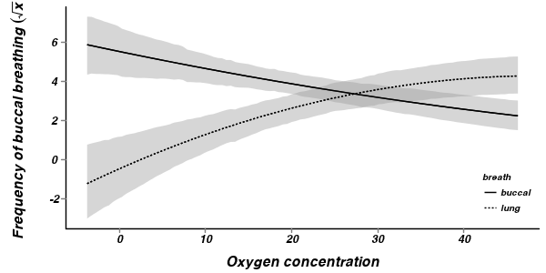
> mullens.mcmc2 <- as.mcmc(mullens.r2jags2$BUGSoutput$sims.matrix)
>
> ##create the prediction model matrix
> xx <- expand.grid(breath = c("buccal", "lung"), O2 = scale(seq(0,
+     50, l = 100), scale = FALSE))
> mullens.mm <- model.matrix(~breath * (O2 + I(O2^2)), xx)
>
> cols <- match(c("g0", "gamma.breath[2]", "beta.o2level", "beta.o2level2",
+     "beta.BreathO2level[2]", "beta.BreathO2level2[2]"), colnames(mullens.mcmc2))
>
> mullens.pred <- predict.mcmc(mcmc = mullens.mcmc2[, cols], mmat = mullens.mm)
> mullens.sum <- data.frame(mullens.mm, mullens.pred, xx)
>
> #mullens.sum <-
> #   data.frame(mullens.mm,means=t(apply(mullens.mcmc2[,cols],2,mean) %*%
> #   t(mullens.mm)),xx)
>
> #coefs <-
> #   fixef(mullens.lme<-lme(SFREQBUC~BREATH*(scale(O2LEVEL,scale=FALSE)+scale(O2LEVEL^2,
> #   scale=FALSE)), random=~1|TOAD, mullens))
> #coefs\t%*% t(mullens.mm)
> #mullens.sum <-
> #   data.frame(mullens.mm,means=t(apply(mullens.mcmc2[,cols],2,mean) %*%
> #   t(mullens.mm)),xx)
> o2.mean <- mean(mullens$O2LEVEL)
>
> p1 <- ggplot(mullens.sum, aes(y = mean, x = O2, group = breath)) +
+     geom_smooth(aes(y = mean, ymin = lower.1, ymax = upper.1, linetype = breath),
+         colour = "black", stat = "identity", show_guide = FALSE) + scale_y_continuous(expression(paste("Frequency of buccal breathing ",
+     (sqrt(x))))) + # trans=trans_new('x2',function(x) {(x^2)},function(x) {sqrt(x)}),
+ # breaks=trans_breaks(function(x) {x^2}, function(x) {sqrt(x)}),
+ # labels=trans_format(function(x) {x^2}, format=format_format()))+
+ scale_x_continuous("Oxygen concentration", trans = trans_new("center",
+     function(x) {
+         x + o2.mean
+     }, function(x) {
+         x - o2.mean
+     }), breaks = trans_breaks(function(x) {
+     x + o2.mean
+ }, function(x) {
+     x - o2.mean
+ }), labels = trans_format(function(x) {
+     x + o2.mean
+ }, format = format_format())) + geom_smooth(aes(linetype = breath), colour = "black",
+     stat = "identity", se = FALSE) + murray_opts + opts(legend.position = c(1,
+     0), legend.justification = c(1, 0))
>
> p1
>
>
- Firstly, the model predicts negative frequencies of buccal breathing by lung breathing toads at very low oxygen concentration. Clearly, this is not logically possible and indicates that the model is a poor representation (either an over or under simplification).
What if we considered O2 level to be a continuous variable?
There are a number of important observations that come out of the previous analysis: