Tutorial 7.4b - Single factor ANOVA (Bayesian)
12 Jan 2018
Overview
Single factor Analysis of Variance (ANOVA, also known as single factor classification) is used to investigate the effect of single factor comprising of two or more groups (treatment levels) from a completely randomized design (see Figures below). Completely randomized refers to the absence of restrictions on the random allocation of experimental or sampling units to factor levels.
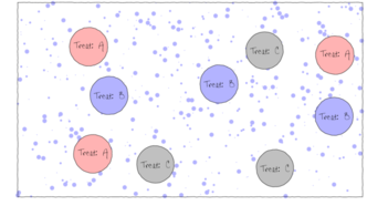
The upper figure depicts a situation in which three types of treatments (A, B and C) are applied to replicate sampling units (quadrats) across the sampling domain (such as the landscape). The underlying (unknown) conditions within this domain are depicted by the variable sized dots. Importantly, the treatments are applied at the scale of the quadrats and the treatments applied to each quadrat do not extend to any other neighbouring quadrats.
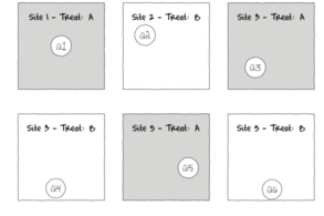
The lower figure represents the situation where the scale of a treatment is far larger than that of a sampling unit (quadrat). This design features two treatments, each replicated three times. Note that additional quadrats within each Site (the scale at which the treatment occurs) would NOT constitute additional replication. Rather, these would be sub-replicates. That is, they would be replicates of the Sites, not the treatments (since the treatments occur at the level of whole sites). In order to genuinely increase the number of replicates, it is necessary to have more Sites.
The random (haphazard) allocation of sampling units (such as quadrats) within the sampling domain (such as population) is appropriate provided either the underlying response is reasonably homogenous throughout the domain, or else, there are a large number of sampling units. If the conditions are relatively hetrogenous (very patchy), then the exact location of the sampling units is likely to be highly influential and may mask any detectable effects of treatments.
Linear model
Recall from Tutorial 7.1 that the linear model for single factor classification is similar to that of multiple linear regression. The linear model can thus be represented by either:
- Means parameterization - in which the regression slopes represent the means of each treatment group and the intercept is removed (to prevent over-parameterization). $$y_{ij}=\beta_1(level_1)_{ij}+\beta_2(level_2)_{ij}+ ... + \varepsilon_{ij}$$ where $\beta_1$ and $\beta_2$ respectively represent the means response of treatment level 1 and 2 respectively. This is often simplified to: $$y_{ij}=\alpha_{i}+ \varepsilon_{ij}$$
- Effects parameterization - the intercept represents a property such as the mean of one of the treatment groups (treatment contrasts) or the overall mean (sum contrasts) etc, and the slope parameters represent effects (differences between each other group and the reference mean for example). $$y_{ij}=\mu+\beta_2(level_2)_{ij}+\beta_3(level_3)_{ij}+ ... + \varepsilon_{ij}$$ where $\mu$ could represent the mean of the first treatment group and $\beta_2$ and $\beta_3$ respectively represent the effects (change from level 1) of level 2 and 3 on the mean response. This is often simplified to: $$y_{ij}=\mu+\alpha_{i}+ \varepsilon_{ij}$$ where $\alpha_1 = 0$.
In a Bayesian framework, it does not really matter whether models are fit with means or effects parameterization since the posterior likelihood can be querried in any way and repeatedly - thus enabling us to explore any specific effects after the model has been fit. Nevertheless, to ease comparisons with frequentist approaches, we will stick with effects paramterisation...
You are strongly encouraged to first view the frequentist tutorial on single factor ANOVA since the issues of exploratory data analysis and parameterization of the linear model are common to both frequentist and Bayesian approaches to single factor ANOVA.
Scenario and Data
Lets say we had set up a natural experiment in which we measured a response ($y$) from 10 sampling units (replicates) from each of 5 treatments. Hence, we have a single categorical factor with 5 levels - we might have five different locations, or five different habitat types or substrates etc. In statistical speak, we have sampled from 5 different populations.
We have then randomly selected 10 independent and random (=representative) units of each population to sample. That is, we have 10 samples (=replicates) of each population.
As this section is mainly about the generation of artificial data (and not specifically about what to do with the data), understanding the actual details are optional and can be safely skipped. Consequently, I have folded (toggled) this section away.
options(width=100)
set.seed(1)
ngroups <- 5  #number of populations
nsample <- 10  #number of reps in each
pop.means <- c(40, 45, 55, 40, 30)  #population mean length
sigma <- 3  #residual standard deviation
n <- ngroups * nsample  #total sample size
eps <- rnorm(n, 0, sigma)  #residuals
x <- gl(ngroups, nsample, n, lab = LETTERS[1:5])  #factor
means <- rep(pop.means, rep(nsample, ngroups))
X <- model.matrix(~x - 1)  #create a design matrix
y <- as.numeric(X %*% pop.means + eps)
data <- data.frame(y, x)
head(data)  #print out the first six rows of the data set
         y x
1 38.12064 A
2 40.55093 A
3 37.49311 A
4 44.78584 A
5 40.98852 A
6 37.53859 A
write.csv(data, "../downloads/data/simpleAnova.csv")
With these sort of data, we are primarily interested in investigating whether there is a relationship between the continuous response variable and the treatment type. Does treatment type effect the response.
Assumptions
- All of the observations are independent - this must be addressed at the design and collection stages. Importantly, to be considered independent replicates, the replicates must be made at the same scale at which the treatment is applied. For example, if the experiment involves subjecting organisms housed in tanks to different water temperatures, then the unit of replication is the individual tanks not the individual organisms in the tanks. The individuals in a tank are strictly not independent with respect to the treatment.
- The response variable (and thus the residuals) should be normally distributed for each sampled population. A boxplot for each treatment is useful for diagnosing major issues with normality.
- The response variable should be equally varied (variance should not be related to mean as these are supposed to be estimated separately) for each treatment. Again, boxplots of each treatment are useful.
Exploratory data analysis
Normality and Homogeneity of variance
boxplot(y ~ x, data)

# OR via ggplot2
library(ggplot2)
ggplot(data, aes(y = y, x = x)) + geom_boxplot() +
    theme_classic()

Conclusions:
- there is no evidence that the response variable is consistently non-normal across all populations - each boxplot is approximately symmetrical
- there is no evidence that variance (as estimated by the height of the boxplots) differs between the five populations. . More importantly, there is no evidence of a relationship between mean and variance - the height of boxplots does not increase with increasing position along the y-axis. Hence it there is no evidence of non-homogeneity
- transform the scale of the response variables (to address normality etc). Note transformations should be applied to the entire response variable (not just those populations that are skewed).
Model fitting or statistical analysis
Consistent with Tutorial 7.2b we will explore Bayesian modelling of single factor ANOVA using a variety of tools (such as MCMCpack, JAGS, RSTAN, RSTANARM and BRMS). Whilst JAGS and RSTAN are extremely flexible and thus allow models to be formulated that contain not only the simple model, but also additional derivatives, the other approaches are more restrictive. Consequently, I will mostly restrict models to just the minimum necessary and all derivatives will instead be calculated in R itself from the returned posteriors.
The observed response ($y_i$) are assumed to be drawn from a normal distribution with a given mean ($\mu$) and standard deviation ($\sigma$). The expected values ($\mu$) are themselves determined by the linear predictor ($\beta_0 + \beta X_i$). In this case, $\beta_0$ represents the mean of the first group and the set of $\beta$'s represent the differences between each other group and the first group.
MCMC sampling requires priors on all parameters. We will employ weakly informative priors. Specifying 'uninformative' priors is always a bit of a balancing act. If the priors are too vague (wide) the MCMC sampler can wander off into nonscence areas of likelihood rather than concentrate around areas of highest likelihood (desired when wanting the outcomes to be largely driven by the data). On the other hand, if the priors are too strong, they may have an influence on the parameters. In such a simple model, this balance is very forgiving - it is for more complex models that prior choice becomes more important.
For this simple model, we will go with zero-centered Gaussian (normal) priors with relatively large standard deviations (100) for both the intercept and the treatment effect and a wide half-cauchy (scale=5) for the standard deviation. $$ \begin{align} y_i &\sim{} N(\mu_i, \sigma)\\ \mu_i &= \beta_0 + \beta X_i\\[1em] \beta_0 &\sim{} N(0,100)\\ \beta &\sim{} N(0,100)\\ \sigma &\sim{} cauchy(0,5)\\ \end{align} $$
library(MCMCpack)
data.mcmcpack <- MCMCregress(y ~ x, data = data)
Specific formulation
For very simple models such as this example, we can write the models as: $$\begin{align} y_i&\sim{}N(\mu_i, \tau)\\ \mu_i &= \beta_0 + \beta X_i\\ \beta_0&\sim{}N(0,1.0{E-6}) \hspace{1cm}\mathsf{non-informative~prior~for~interept}\\ \beta_j&\sim{}N(0,1.0{E-6}) \hspace{1cm}\mathsf{non-informative~prior~for~partial~slopes}\\ \tau &= 1/\sigma^2\\ \sigma&\sim{}U(0,100)\\ \end{align} $$
Define the model
Note the following example as group means calculated as derived posteriors
modelString = "
  model {
  #Likelihood
  for (i in 1:n) {
  y[i]~dnorm(mean[i],tau.res)
  mean[i] <- alpha+beta[x[i]]
  }

  #Priors and derivatives
  alpha ~ dnorm(0,1.0E-6)
  beta[1] <- 0
  for (i in 2:ngroups) {
  beta[i] ~ dnorm(0, 1.0E-6) #prior
  }
  sigma.res ~ dunif(0, 100)
  tau.res <- 1 / (sigma.res * sigma.res)
  sigma.group <- sd(beta[])

  #Group mean posteriors (derivatives)
  for (i in 1:ngroups) {
  Group.means[i] <- beta[i]+alpha
  }
  }
  "
Arrange the data as a list (as required by BUGS). As input, JAGS will need to be supplied with:
- the response variable (y)
- a numeric representation of the predictor variable (x)
- the total number of observed items (n)
- the number of groups
data.list <- with(data, list(y = y, x = as.numeric(x), n = nrow(data),
    ngroups = length(levels(data$x))))
Define the MCMC chain parameters
Next we should define the behavioural parameters of the MCMC sampling chains. Include the following:
- the nodes (estimated parameters) to monitor (return samples for)
- the number of MCMC chains (3)
- the number of burnin steps (1000)
- the thinning factor (10)
- the number of MCMC iterations - determined by the number of samples to save, the rate of thinning and the number of chains
params <- c("alpha", "beta", "sigma", "Group.means")
nChains = 3
burnInSteps = 3000
thinSteps = 10
numSavedSteps = 15000  #across all chains
nIter = ceiling(burnInSteps + (numSavedSteps * thinSteps)/nChains)
nIter
[1] 53000
Fit the model
Now run the JAGS code via the R2jags interface. Note that the first time jags is run after the R2jags package is loaded, it is often necessary to run any kind of randomization function just to initiate the .Random.seed variable.
## load the R2jags package
library(R2jags)
data.r2jags <- jags(data = data.list, inits = NULL, parameters.to.save = params,
    model.file = textConnection(modelString), n.chains = nChains, n.iter = nIter,
    n.burnin = burnInSteps, n.thin = thinSteps)
Compiling model graph
   Resolving undeclared variables
   Allocating nodes
Graph information:
   Observed stochastic nodes: 50
   Unobserved stochastic nodes: 6
   Total graph size: 137

Initializing model
print(data.r2jags)
Inference for Bugs model at "5", fit using jags,
 3 chains, each with 53000 iterations (first 3000 discarded), n.thin = 10
 n.sims = 15000 iterations saved
               mu.vect sd.vect    2.5%     25%     50%     75%   97.5%  Rhat n.eff
Group.means[1]  40.390   0.847  38.688  39.838  40.389  40.955  42.065 1.001 15000
Group.means[2]  45.742   0.840  44.110  45.174  45.739  46.295  47.417 1.001 13000
Group.means[3]  54.591   0.844  52.961  54.026  54.589  55.141  56.299 1.001 15000
Group.means[4]  40.370   0.844  38.749  39.795  40.366  40.929  42.049 1.001  7700
Group.means[5]  30.396   0.844  28.747  29.833  30.394  30.949  32.057 1.001 15000
alpha           40.390   0.847  38.688  39.838  40.389  40.955  42.065 1.001 15000
beta[1]          0.000   0.000   0.000   0.000   0.000   0.000   0.000 1.000     1
beta[2]          5.353   1.196   2.982   4.568   5.355   6.144   7.713 1.001 14000
beta[3]         14.201   1.190  11.894  13.410  14.195  14.980  16.597 1.001 15000
beta[4]         -0.020   1.196  -2.342  -0.823  -0.029   0.772   2.364 1.001 15000
beta[5]         -9.994   1.194 -12.317 -10.789 -10.004  -9.198  -7.615 1.001 15000
deviance       237.628   3.789 232.446 234.858 236.901 239.639 247.035 1.001 15000

For each parameter, n.eff is a crude measure of effective sample size,
and Rhat is the potential scale reduction factor (at convergence, Rhat=1).

DIC info (using the rule, pD = var(deviance)/2)
pD = 7.2 and DIC = 244.8
DIC is an estimate of expected predictive error (lower deviance is better).
data.mcmc.list <- as.mcmc(data.r2jags)
Model matrix formulation
For very simple models such as this example, we can write the models as: $$\begin{align} y_i&\sim{}N(\mu_i, \tau)\\ \mu_i &= \beta_0 + \beta X_i\\ \beta_0&\sim{}N(0,1.0{E-6}) \hspace{1cm}\mathsf{non-informative~prior~for~interept}\\ \beta_j&\sim{}N(0,1.0{E-6}) \hspace{1cm}\mathsf{non-informative~prior~for~partial~slopes}\\ \tau &= 1/\sigma^2\\ \sigma&\sim{}U(0,100)\\ \end{align} $$
Define the model
modelString = "
  model {
  #Likelihood
  for (i in 1:n) {
  y[i]~dnorm(mean[i],tau)
  mean[i] <- inprod(beta[],X[i,])
  }
  #Priors
  for (i in 1:ngroups) {
  beta[i] ~ dnorm(0, 1.0E-6)
  }
  sigma ~ dunif(0, 100)
  tau <- 1 / (sigma * sigma)
  }
  "
Define the data
Arrange the data as a list (as required by BUGS). As input, JAGS will need to be supplied with:
- the response variable (y)
- the predictor model matrix (X)
- the total number of observed items (n)
- the number of predictor terms (nX)
X <- model.matrix(~x, data)
data.list <- with(data, list(y = y, X = X, n = nrow(data), ngroups = ncol(X)))
Define the MCMC chain parameters
Next we should define the behavioural parameters of the MCMC sampling chains. Include the following:
- the nodes (estimated parameters) to monitor (return samples for)
- the number of MCMC chains (3)
- the number of burnin steps (1000)
- the thinning factor (10)
- the number of MCMC iterations - determined by the number of samples to save, the rate of thinning and the number of chains
params <- c("beta", "sigma")
nChains = 3
burnInSteps = 3000
thinSteps = 10
numSavedSteps = 15000  #across all chains
nIter = ceiling(burnInSteps + (numSavedSteps * thinSteps)/nChains)
nIter
[1] 53000
Fit the model
Now run the JAGS code via the R2jags interface. Note that the first time jags is run after the R2jags package is loaded, it is often necessary to run any kind of randomization function just to initiate the .Random.seed variable.
data.r2jags <- jags(data = data.list, inits = NULL, parameters.to.save = params,
    model.file = textConnection(modelString), n.chains = nChains, n.iter = nIter,
    n.burnin = burnInSteps, n.thin = thinSteps)
Compiling model graph
   Resolving undeclared variables
   Allocating nodes
Graph information:
   Observed stochastic nodes: 50
   Unobserved stochastic nodes: 6
   Total graph size: 380

Initializing model
print(data.r2jags)
Inference for Bugs model at "5", fit using jags,
 3 chains, each with 53000 iterations (first 3000 discarded), n.thin = 10
 n.sims = 15000 iterations saved
         mu.vect sd.vect    2.5%     25%     50%     75%   97.5%  Rhat n.eff
beta[1]   40.387   0.841  38.745  39.825  40.386  40.944  42.037 1.001 15000
beta[2]    5.363   1.190   3.058   4.556   5.363   6.164   7.710 1.001 15000
beta[3]   14.204   1.183  11.866  13.419  14.204  14.998  16.518 1.001 15000
beta[4]   -0.042   1.192  -2.358  -0.837  -0.031   0.745   2.283 1.001  8400
beta[5]   -9.987   1.193 -12.348 -10.780  -9.977  -9.199  -7.645 1.001 15000
sigma      2.646   0.287   2.157   2.447   2.619   2.817   3.284 1.001 15000
deviance 237.605   3.796 232.404 234.815 236.902 239.573 247.009 1.001 15000

For each parameter, n.eff is a crude measure of effective sample size,
and Rhat is the potential scale reduction factor (at convergence, Rhat=1).

DIC info (using the rule, pD = var(deviance)/2)
pD = 7.2 and DIC = 244.8
DIC is an estimate of expected predictive error (lower deviance is better).
data.mcmc.list <- as.mcmc(data.r2jags)
Whilst Gibbs sampling provides an elegantly simple MCMC sampling routine, very complex hierarchical models can take enormous numbers of iterations (often prohibitory large) to converge on a stable posterior distribution.
To address this, Andrew Gelman (and other collaborators) have implemented a variation on Hamiltonian Monte Carlo (HMC: a sampler that selects subsequent samples in a way that reduces the correlation between samples, thereby speeding up convergence) called the No-U-Turn (NUTS) sampler. All of these developments are brought together into a tool called Stan ("Sampling Through Adaptive Neighborhoods").
By design (to appeal to the vast BUGS users), Stan models are defined in a manner reminiscent of BUGS. Stan first converts these models into C++ code which is then compiled to allow very rapid computation.
Consistent with the use of C++, the model must be accompanied by variable declarations for all inputs and parameters.
One important difference between Stan and JAGS is that whereas BUGS (and thus JAGS) use precision rather than variance, Stan uses variance.
Stan itself is a stand-alone command line application. However, conveniently, the authors of Stan have also developed an R interface to Stan called Rstan which can be used much like R2jags.
Model matrix formulation
The minimum model in Stan required to fit the above simple regression follows. Note the following modifications from the model defined in JAGS:- the normal distribution is defined by variance rather than precision
- rather than using a uniform prior for sigma, I am using a half-Cauchy
We now translate the likelihood model into STAN code.
$$\begin{align}
y_i&\sim{}N(\mu_i, \sigma)\\
\mu_i &= \beta_0+\beta X_i\\
\beta_0&\sim{}N(0,100)\\
\beta&\sim{}N(0,100)\\
\sigma&\sim{}Cauchy(0,5)\\
\end{align}
$$
Define the model
modelString = "
  data {
  int<lower=1> n;
  int<lower=1> nX;
  vector [n] y;
  matrix [n,nX] X;
  }
  parameters {
  vector[nX] beta;
  real<lower=0> sigma;
  }
  transformed parameters {
  vector[n] mu;

  mu = X*beta;
  }
  model {
  #Likelihood
  y~normal(mu,sigma);

  #Priors
  beta ~ normal(0,1000);
  sigma~cauchy(0,5);
  }
  generated quantities {
  vector[n] log_lik;

  for (i in 1:n) {
  log_lik[i] = normal_lpdf(y[i] | mu[i], sigma);
  }
  }
  "
Define the data
Arrange the data as a list (as required by BUGS). As input, JAGS will need to be supplied with:
- the response variable (y)
- the predictor model matrix (X)
- the total number of observed items (n)
- the number of predictor terms (nX)
Xmat <- model.matrix(~x, data)
data.list <- with(data, list(y = y, X = Xmat, nX = ncol(Xmat), n = nrow(data)))
Fit the model
Now run the JAGS code via the R2jags interface. Note that the first time jags is run after the R2jags package is loaded, it is often necessary to run any kind of randomization function just to initiate the .Random.seed variable.
## load the rstan package
library(rstan)
data.rstan <- stan(data = data.list, model_code = modelString, chains = 3,
    iter = 2000, warmup = 500, thin = 3)
In file included from /usr/local/lib/R/site-library/BH/include/boost/config.hpp:39:0,
                 from /usr/local/lib/R/site-library/BH/include/boost/math/tools/config.hpp:13,
                 from /usr/local/lib/R/site-library/StanHeaders/include/stan/math/rev/core/var.hpp:7,
                 from /usr/local/lib/R/site-library/StanHeaders/include/stan/math/rev/core/gevv_vvv_vari.hpp:5,
                 from /usr/local/lib/R/site-library/StanHeaders/include/stan/math/rev/core.hpp:12,
                 from /usr/local/lib/R/site-library/StanHeaders/include/stan/math/rev/mat.hpp:4,
                 from /usr/local/lib/R/site-library/StanHeaders/include/stan/math.hpp:4,
                 from /usr/local/lib/R/site-library/StanHeaders/include/src/stan/model/model_header.hpp:4,
                 from file1c233b59b6c8.cpp:8:
/usr/local/lib/R/site-library/BH/include/boost/config/compiler/gcc.hpp:186:0: warning: "BOOST_NO_CXX11_RVALUE_REFERENCES" redefined
 #  define BOOST_NO_CXX11_RVALUE_REFERENCES
 ^
<command-line>:0:0: note: this is the location of the previous definition

SAMPLING FOR MODEL '3b057d3d81cbed2078ce678376a94574' NOW (CHAIN 1).

Gradient evaluation took 1.5e-05 seconds
1000 transitions using 10 leapfrog steps per transition would take 0.15 seconds.
Adjust your expectations accordingly!


Iteration:    1 / 2000 [  0%]  (Warmup)
Iteration:  200 / 2000 [ 10%]  (Warmup)
Iteration:  400 / 2000 [ 20%]  (Warmup)
Iteration:  501 / 2000 [ 25%]  (Sampling)
Iteration:  700 / 2000 [ 35%]  (Sampling)
Iteration:  900 / 2000 [ 45%]  (Sampling)
Iteration: 1100 / 2000 [ 55%]  (Sampling)
Iteration: 1300 / 2000 [ 65%]  (Sampling)
Iteration: 1500 / 2000 [ 75%]  (Sampling)
Iteration: 1700 / 2000 [ 85%]  (Sampling)
Iteration: 1900 / 2000 [ 95%]  (Sampling)
Iteration: 2000 / 2000 [100%]  (Sampling)

 Elapsed Time: 0.037412 seconds (Warm-up)
               0.084862 seconds (Sampling)
               0.122274 seconds (Total)


SAMPLING FOR MODEL '3b057d3d81cbed2078ce678376a94574' NOW (CHAIN 2).

Gradient evaluation took 1.1e-05 seconds
1000 transitions using 10 leapfrog steps per transition would take 0.11 seconds.
Adjust your expectations accordingly!


Iteration:    1 / 2000 [  0%]  (Warmup)
Iteration:  200 / 2000 [ 10%]  (Warmup)
Iteration:  400 / 2000 [ 20%]  (Warmup)
Iteration:  501 / 2000 [ 25%]  (Sampling)
Iteration:  700 / 2000 [ 35%]  (Sampling)
Iteration:  900 / 2000 [ 45%]  (Sampling)
Iteration: 1100 / 2000 [ 55%]  (Sampling)
Iteration: 1300 / 2000 [ 65%]  (Sampling)
Iteration: 1500 / 2000 [ 75%]  (Sampling)
Iteration: 1700 / 2000 [ 85%]  (Sampling)
Iteration: 1900 / 2000 [ 95%]  (Sampling)
Iteration: 2000 / 2000 [100%]  (Sampling)

 Elapsed Time: 0.035185 seconds (Warm-up)
               0.077264 seconds (Sampling)
               0.112449 seconds (Total)


SAMPLING FOR MODEL '3b057d3d81cbed2078ce678376a94574' NOW (CHAIN 3).

Gradient evaluation took 1.9e-05 seconds
1000 transitions using 10 leapfrog steps per transition would take 0.19 seconds.
Adjust your expectations accordingly!


Iteration:    1 / 2000 [  0%]  (Warmup)
Iteration:  200 / 2000 [ 10%]  (Warmup)
Iteration:  400 / 2000 [ 20%]  (Warmup)
Iteration:  501 / 2000 [ 25%]  (Sampling)
Iteration:  700 / 2000 [ 35%]  (Sampling)
Iteration:  900 / 2000 [ 45%]  (Sampling)
Iteration: 1100 / 2000 [ 55%]  (Sampling)
Iteration: 1300 / 2000 [ 65%]  (Sampling)
Iteration: 1500 / 2000 [ 75%]  (Sampling)
Iteration: 1700 / 2000 [ 85%]  (Sampling)
Iteration: 1900 / 2000 [ 95%]  (Sampling)
Iteration: 2000 / 2000 [100%]  (Sampling)

 Elapsed Time: 0.036548 seconds (Warm-up)
               0.061915 seconds (Sampling)
               0.098463 seconds (Total)
print(data.rstan, par = c("beta", "sigma"))
Inference for Stan model: 3b057d3d81cbed2078ce678376a94574.
3 chains, each with iter=2000; warmup=500; thin=3;
post-warmup draws per chain=500, total post-warmup draws=1500.

         mean se_mean   sd   2.5%    25%   50%   75% 97.5% n_eff Rhat
beta[1] 40.40    0.02 0.84  38.75  39.85 40.38 40.95 42.06  1142    1
beta[2]  5.36    0.03 1.20   3.04   4.53  5.38  6.17  7.80  1302    1
beta[3] 14.21    0.03 1.19  11.88  13.37 14.20 15.01 16.68  1168    1
beta[4] -0.04    0.03 1.19  -2.35  -0.83 -0.06  0.79  2.23  1202    1
beta[5] -9.96    0.03 1.17 -12.14 -10.78 -9.95 -9.13 -7.76  1234    1
sigma    2.65    0.01 0.29   2.14   2.44  2.63  2.83  3.23  1332    1

Samples were drawn using NUTS(diag_e) at Mon Aug 28 20:56:23 2017.
For each parameter, n_eff is a crude measure of effective sample size,
and Rhat is the potential scale reduction factor on split chains (at
convergence, Rhat=1).
The STAN team has put together pre-compiled modules (functions) to make specifying and applying STAN models much simpler. Each function offers a consistent interface that is Also reminiscent of major frequentist linear modelling routines in R.
Whilst it is not necessary to specify priors when using rstanarm functions (as defaults will be generated), there is no guarantee that the routines for determining these defaults will persist over time. Furthermore, it is always better to define your own priors if for no other reason that it forces you to thing about what you re doing. Consistent with the pure STAN version, we will employ the following priors:
- weakly informative Gaussian prior for the intercept $\beta_0 \sim{} N(0, 100)$
- weakly informative Gaussian prior for the treatment effect $\beta_1 \sim{} N(0, 100)$
- half-cauchy prior for the variance $\sigma \sim{} Cauchy(0, 5)$
Note, I am using the refresh=0 option so as to suppress the larger regular output in the interest of keeping output to what is necessary for this tutorial. When running outside of a tutorial context, the regular verbose output is useful as it provides a way to gauge progress.
library(rstanarm)
library(broom)
library(coda)
data.rstanarm = stan_glm(y ~ x, data = data, iter = 2000, warmup = 500,
    chains = 3, thin = 2, refresh = 0, prior_intercept = normal(0, 100),
    prior = normal(0, 100), prior_aux = cauchy(0, 2))
Gradient evaluation took 4.6e-05 seconds
1000 transitions using 10 leapfrog steps per transition would take 0.46 seconds.
Adjust your expectations accordingly!


 Elapsed Time: 0.121397 seconds (Warm-up)
               0.251909 seconds (Sampling)
               0.373306 seconds (Total)


Gradient evaluation took 1.2e-05 seconds
1000 transitions using 10 leapfrog steps per transition would take 0.12 seconds.
Adjust your expectations accordingly!


 Elapsed Time: 0.117929 seconds (Warm-up)
               0.159803 seconds (Sampling)
               0.277732 seconds (Total)


Gradient evaluation took 1.7e-05 seconds
1000 transitions using 10 leapfrog steps per transition would take 0.17 seconds.
Adjust your expectations accordingly!


 Elapsed Time: 0.207204 seconds (Warm-up)
               0.153911 seconds (Sampling)
               0.361115 seconds (Total)
print(data.rstanarm)
stan_glm
 family:  gaussian [identity]
 formula: y ~ x
------

Estimates:
            Median MAD_SD
(Intercept)  40.4    0.8
xB            5.3    1.2
xC           14.2    1.2
xD            0.0    1.1
xE          -10.0    1.1
sigma         2.6    0.3

Sample avg. posterior predictive
distribution of y (X = xbar):
         Median MAD_SD
mean_PPD 42.3    0.5

------
For info on the priors used see help('prior_summary.stanreg').
tidyMCMC(data.rstanarm, conf.int = TRUE, conf.method = "HPDinterval")
         term    estimate std.error   conf.low conf.high
1 (Intercept) 40.37013202 0.8369156  38.641206 41.904030
2          xB  5.35134132 1.1832942   3.008367  7.741613
3          xC 14.23032089 1.1924590  11.961883 16.741929
4          xD  0.01681653 1.1703009  -2.498183  2.092344
5          xE -9.99518905 1.1917167 -12.239427 -7.563808
6       sigma  2.65469957 0.2833189   2.149518  3.229648
The brms package serves a similar goal to the rstanarm package - to provide a simple user interface to STAN. However, unlike the rstanarm implementation, brms simply converts the formula, data, priors and family into STAN model code and data before executing stan with those elements.
Whilst it is not necessary to specify priors when using brms functions (as defaults will be generated), there is no guarantee that the routines for determining these defaults will persist over time. Furthermore, it is always better to define your own priors if for no other reason that it forces you to thing about what you are doing. Consistent with the pure STAN version, we will employ the following priors:
- weakly informative Gaussian prior for the intercept $\beta_0 \sim{} N(0, 100)$
- weakly informative Gaussian prior for the treatment effect $\beta_1 \sim{} N(0, 100)$
- half-cauchy prior for the variance $\sigma \sim{} Cauchy(0, 5)$
Note, I am using the refresh=0. option so as to suppress the larger regular output in the interest of keeping output to what is necessary for this tutorial. When running outside of a tutorial context, the regular verbose output is useful as it provides a way to gauge progress.
library(brms)
library(broom)
library(coda)
data.brms = brm(y ~ x, data = data, iter = 2000, warmup = 500, chains = 3,
    thin = 2, refresh = 0, prior = c(prior(normal(0, 100), class = "Intercept"),
        prior(normal(0, 100), class = "b"), prior(cauchy(0, 5), class = "sigma")))
Gradient evaluation took 2.1e-05 seconds
1000 transitions using 10 leapfrog steps per transition would take 0.21 seconds.
Adjust your expectations accordingly!


 Elapsed Time: 0.033766 seconds (Warm-up)
               0.050702 seconds (Sampling)
               0.084468 seconds (Total)


Gradient evaluation took 8e-06 seconds
1000 transitions using 10 leapfrog steps per transition would take 0.08 seconds.
Adjust your expectations accordingly!


 Elapsed Time: 0.03249 seconds (Warm-up)
               0.053189 seconds (Sampling)
               0.085679 seconds (Total)


Gradient evaluation took 6e-06 seconds
1000 transitions using 10 leapfrog steps per transition would take 0.06 seconds.
Adjust your expectations accordingly!


 Elapsed Time: 0.034406 seconds (Warm-up)
               0.061338 seconds (Sampling)
               0.095744 seconds (Total)
print(data.brms)
 Family: gaussian(identity)
Formula: y ~ x
   Data: data (Number of observations: 50)
Samples: 3 chains, each with iter = 2000; warmup = 500; thin = 2;
         total post-warmup samples = 2250
    ICs: LOO = NA; WAIC = NA; R2 = NA

Population-Level Effects:
          Estimate Est.Error l-95% CI u-95% CI Eff.Sample Rhat
Intercept    40.37      0.85    38.73    41.99       1830    1
xB            5.38      1.20     2.97     7.77       1834    1
xC           14.22      1.19    11.90    16.69       1816    1
xD            0.03      1.18    -2.30     2.33       1822    1
xE           -9.96      1.20   -12.30    -7.65       1575    1

Family Specific Parameters:
      Estimate Est.Error l-95% CI u-95% CI Eff.Sample Rhat
sigma     2.63      0.29     2.13     3.24       1967    1

Samples were drawn using sampling(NUTS). For each parameter, Eff.Sample
is a crude measure of effective sample size, and Rhat is the potential
scale reduction factor on split chains (at convergence, Rhat = 1).
tidyMCMC(data.brms, conf.int = TRUE, conf.method = "HPDinterval")
         term   estimate std.error   conf.low conf.high
1 b_Intercept 40.3681829 0.8453842  38.733357 41.995095
2        b_xB  5.3835983 1.1963019   3.133155  7.926054
3        b_xC 14.2246055 1.1934948  12.002788 16.737062
4        b_xD  0.0322263 1.1761590  -2.398031  2.192691
5        b_xE -9.9603899 1.1972640 -12.385544 -7.745285
6       sigma  2.6319625 0.2902885   2.123581  3.222859
MCMC diagnostics
In addition to the regular model diagnostic checks (such as residual plots), for Bayesian analyses, it is necessary to explore the characteristics of the MCMC chains and the sampler in general. Recall that the purpose of MCMC sampling is to replicate the posterior distribution of the model likelihood and priors by drawing a known number of samples from this posterior (thereby formulating a probability distribution). This is only reliable if the MCMC samples accurately reflect the posterior.
Unfortunately, since we only know the posterior in the most trivial of circumstances, it is necessary to rely on indirect measures of how accurately the MCMC samples are likely to reflect the likelihood. I will breifly outline the most important diagnostics, however, please refer to Tutorial 4.3, Secton 3.1: Markov Chain Monte Carlo sampling for a discussion of these diagnostics.
- Traceplots for each parameter illustrate the MCMC sample values after each successive
iteration along the chain. Bad chain mixing (characterized by any sort of pattern) suggests
that the MCMC sampling chains may not have completely traversed all features of the posterior
distribution and that more iterations are required to ensure the distribution has been accurately
represented.

- Autocorrelation plot for each paramter illustrate the degree of correlation between
MCMC samples separated by different lags. For example, a lag of 0 represents the degree of
correlation between each MCMC sample and itself (obviously this will be a correlation of 1).
A lag of 1 represents the degree of correlation between each MCMC sample and the next sample along the Chain
and so on. In order to be able to generate unbiased estimates of parameters, the MCMC samples should be
independent (uncorrelated). In the figures below, this would be violated in the top autocorrelation plot and met in the bottom
autocorrelation plot.


- Rhat statistic for each parameter provides a measure of sampling efficiency/effectiveness. Ideally, all values should be less than 1.05. If there are values of 1.05 or greater it suggests that the sampler was not very efficient or effective. Not only does this mean that the sampler was potentiall slower than it could have been, more importantly, it could indicate that the sampler spent time sampling in a region of the likelihood that is less informative. Such a situation can arise from either a misspecified model or overly vague priors that permit sampling in otherwise nonscence parameter space.
Prior to inspecting any summaries of the parameter estimates, it is prudent to inspect a range of chain convergence diagnostics.
- Trace plots
View trace plotsTrace plots show no evidence that the chains have not reasonably traversed the entire multidimensional parameter space.
library(MCMCpack)
plot(data.mcmcpack)


- Raftery diagnostic
View Raftery diagnosticThe Raftery diagnostics estimate that we would require about 3900 samples to reach the specified level of confidence in convergence. As we have 10,000 samples, we can be confidence that convergence has occurred.
library(MCMCpack)
raftery.diag(data.mcmcpack)
Quantile (q) = 0.025 Accuracy (r) = +/- 0.005 Probability (s) = 0.95 Burn-in Total Lower bound Dependence (M) (N) (Nmin) factor (I) (Intercept) 2 3865 3746 1.030 xB 2 3771 3746 1.010 xC 2 3802 3746 1.010 xD 2 3929 3746 1.050 xE 2 3865 3746 1.030 sigma2 2 3741 3746 0.999 - Autocorrelation diagnostic
View autocorrelationsA lag of 1 appears to be mainly sufficient to avoid autocorrelation.
library(MCMCpack)
autocorr.diag(data.mcmcpack)
        (Intercept)            xB           xC           xD           xE       sigma2
Lag 0   1.000000000  1.000000e+00  1.000000000  1.000000000  1.000000000  1.000000000
Lag 1  -0.002026451 -2.584595e-03  0.002845588  0.001221385 -0.001192370  0.113629174
Lag 5   0.005186105  6.716212e-05 -0.005876489  0.001195213 -0.005830629 -0.002827759
Lag 10 -0.004695655 -3.112666e-03 -0.017000405 -0.016469962 -0.005235883 -0.008952653
Lag 50  0.001227380  1.032229e-02 -0.003024500 -0.001542249 -0.004604603 -0.014062511
Again, prior to examining the summaries, we should have explored the convergence diagnostics.
library(coda)
data.mcmc = as.mcmc(data.r2jags)
- Trace plots
Trace plots show no evidence that the chains have not reasonably traversed the entire multidimensional parameter space.
plot(data.mcmc)


When there are a lot of parameters, this can result in a very large number of traceplots. To focus on just certain parameters (such as $\beta$s)
preds <- c("beta[1]", "beta[2]", "beta[3]", "beta[4]", "beta[5]")
plot(as.mcmc(data.r2jags)[, preds])


- Raftery diagnostic
The Raftery diagnostics for each chain estimate that we would require no more than 5000 samples to reach the specified level of confidence in convergence. As we have 16,667 samples, we can be confidence that convergence has occurred.
raftery.diag(data.mcmc)
[[1]] Quantile (q) = 0.025 Accuracy (r) = +/- 0.005 Probability (s) = 0.95 Burn-in Total Lower bound Dependence (M) (N) (Nmin) factor (I) beta[1] 20 36800 3746 9.82 beta[2] 20 39300 3746 10.50 beta[3] 20 36800 3746 9.82 beta[4] 20 38030 3746 10.20 beta[5] 20 36200 3746 9.66 deviance 20 37410 3746 9.99 sigma 20 36800 3746 9.82 [[2]] Quantile (q) = 0.025 Accuracy (r) = +/- 0.005 Probability (s) = 0.95 Burn-in Total Lower bound Dependence (M) (N) (Nmin) factor (I) beta[1] 20 36810 3746 9.83 beta[2] 20 38030 3746 10.20 beta[3] 20 36800 3746 9.82 beta[4] 20 36800 3746 9.82 beta[5] 20 38660 3746 10.30 deviance 20 38030 3746 10.20 sigma 20 38660 3746 10.30 [[3]] Quantile (q) = 0.025 Accuracy (r) = +/- 0.005 Probability (s) = 0.95 Burn-in Total Lower bound Dependence (M) (N) (Nmin) factor (I) beta[1] 20 35610 3746 9.51 beta[2] 20 39950 3746 10.70 beta[3] 20 37410 3746 9.99 beta[4] 20 36200 3746 9.66 beta[5] 20 38660 3746 10.30 deviance 20 38030 3746 10.20 sigma 20 38030 3746 10.20 - Autocorrelation diagnostic
A lag of 10 appears to be sufficient to avoid autocorrelation (poor mixing).
autocorr.diag(data.mcmc)
             beta[1]       beta[2]      beta[3]      beta[4]       beta[5]      deviance
Lag 0    1.000000000  1.0000000000  1.000000000  1.000000000  1.0000000000  1.0000000000
Lag 10   0.000511858  0.0141941964  0.003049321 -0.001101961 -0.0136748526  0.0073553829
Lag 50  -0.008312100 -0.0097313263 -0.003298050  0.003033837  0.0006659111  0.0002969917
Lag 100 -0.006018466 -0.0008556030 -0.009141989 -0.001865391  0.0025599386 -0.0034075443
Lag 500  0.014270778  0.0005677835  0.012646093  0.012218425 -0.0020017030  0.0002759488
              sigma
Lag 0   1.000000000
Lag 10  0.002197296
Lag 50  0.010001090
Lag 100 0.002718464
Lag 500 0.007906380
Again, prior to examining the summaries, we should have explored the convergence diagnostics. There are numerous ways of working with STAN model fits (for exploring diagnostics and summarization).
- extract the mcmc samples and convert them into a mcmc.list to leverage the various coda routines
- use the numerous routines that come with the rstan package
- use the routines that come with the bayesplot package
- explore the diagnostics interactively via shinystan
- via coda
- Traceplots
- Autocorrelation
Trace plots show no evidence that the chains have not reasonably traversed the entire multidimensional parameter space.library(coda) s = as.array(data.rstan) wch = grep("beta", dimnames(s)$parameters) s = s[, , wch] mcmc <- do.call(mcmc.list, plyr:::alply(s[, , -(length(s[1, 1, ]))], 2, as.mcmc)) plot(mcmc)
 Trace plots show no evidence that the chains have not reasonably traversed the entire multidimensional parameter space.
library(coda)
s = as.array(data.rstan)
wch = grep("beta", dimnames(s)$parameters)
s = s[, , wch]
mcmc <- do.call(mcmc.list, plyr:::alply(s[, , -(length(s[1, 1, ]))], 2, as.mcmc))
autocorr.diag(mcmc)
             beta[1]    beta[2]      beta[3]       beta[4]
Lag 0   1.000000e+00 1.00000000  1.000000000  1.0000000000
Lag 1   8.980238e-02 0.03370305  0.086635647  0.0373446611
Lag 5  -2.807365e-02 0.02098545  0.003301172  0.0004472765
Lag 10 -7.017194e-03 0.01037456 -0.003796991 -0.0008328611
Lag 50 -6.760447e-05 0.01494083 -0.018636469  0.0418145402
- via rstan
- Traceplots
Trace plots show no evidence that the chains have not reasonably traversed the entire multidimensional parameter space.
stan_trace(data.rstan)

- Raftery diagnostic
The Raftery diagnostics for each chain estimate that we would require no more than 5000 samples to reach the specified level of confidence in convergence. As we have 16,667 samples, we can be confidence that convergence has occurred.
raftery.diag(data.rstan)
Quantile (q) = 0.025
Accuracy (r) = +/- 0.005
Probability (s) = 0.95

You need a sample size of at least 3746 with these values of q, r and s
- Autocorrelation diagnostic
A lag of 2 appears broadly sufficient to avoid autocorrelation (poor mixing).
stan_ac(data.rstan)

- Rhat values. These values are a measure of sampling efficiency/effectiveness. Ideally, all values should be less than 1.05.
If there are values of 1.05 or greater it suggests that the sampler was not very efficient or effective. Not only does this
mean that the sampler was potentiall slower than it could have been, more importantly, it could indicate that the sampler spent time sampling
in a region of the likelihood that is less informative. Such a situation can arise from either a misspecified model or
overly vague priors that permit sampling in otherwise nonscence parameter space.
In this instance, all rhat values are well below 1.05 (a good thing).
stan_rhat(data.rstan)

- Another measure of sampling efficiency is Effective Sample Size (ess).
ess indicate the number samples (or proportion of samples that the sampling algorithm deamed effective. The sampler rejects samples
on the basis of certain criterion and when it does so, the previous sample value is used. Hence while the MCMC sampling chain
may contain 1000 samples, if there are only 10 effective samples (1%), the estimated properties are not likely to be reliable.
In this instance, most of the parameters have reasonably high effective samples and thus there is likely to be a good range of values from which to estimate paramter properties.
stan_ess(data.rstan)

- Traceplots
- via bayesplot
- Trace plots and density plots
Trace plots show no evidence that the chains have not reasonably traversed the entire multidimensional parameter space.
library(bayesplot)
mcmc_trace(as.matrix(data.rstan), regex_pars = "beta|sigma")

library(bayesplot)
mcmc_combo(as.matrix(data.rstan), regex_pars = "beta|sigma")

- Density plots
Density plots sugggest mean or median would be appropriate to describe the fixed posteriors and median is appropriate for the sigma posterior.
library(bayesplot)
mcmc_dens(as.matrix(data.rstan), regex_pars = "beta|sigma")

- Trace plots and density plots
- via shinystan
library(shinystan)
launch_shinystan(data.rstan)
- It is worth exploring the influence of our priors.
Again, prior to examining the summaries, we should have explored the convergence diagnostics. There are numerous ways of working with STANARM model fits (for exploring diagnostics and summarization).
- extract the mcmc samples and convert them into a mcmc.list to leverage the various coda routines
- use the numerous routines that come with the rstan package
- use the routines that come with the bayesplot package
- explore the diagnostics interactively via shinystan
- via coda
- Traceplots
- Autocorrelation
Trace plots show no evidence that the chains have not reasonably traversed the entire multidimensional parameter space.library(coda) s = as.array(data.rstanarm) mcmc <- do.call(mcmc.list, plyr:::alply(s[, , -(length(s[1, 1, ]))], 2, as.mcmc)) plot(mcmc)

 Trace plots show no evidence that the chains have not reasonably traversed the entire multidimensional parameter space.
library(coda)
s = as.array(data.rstanarm)
mcmc <- do.call(mcmc.list, plyr:::alply(s[, , -(length(s[1, 1, ]))], 2, as.mcmc))
autocorr.diag(mcmc)
        (Intercept)          xB          xC          xD            xE
Lag 0   1.000000000  1.00000000  1.00000000 1.000000000  1.0000000000
Lag 1   0.027385218  0.01674547  0.01421235 0.006356097  0.0192142041
Lag 5   0.005678036  0.02326828  0.01627096 0.020524683 -0.0148176836
Lag 10 -0.015002246  0.01468946 -0.03007735 0.007219375  0.0074786588
Lag 50 -0.024405944 -0.03054356  0.01621183 0.000803842 -0.0001606121
- via rstan
- Traceplots
Trace plots show no evidence that the chains have not reasonably traversed the entire multidimensional parameter space.
stan_trace(data.rstanarm)

- Raftery diagnostic
The Raftery diagnostics for each chain estimate that we would require no more than 5000 samples to reach the specified level of confidence in convergence. As we have 16,667 samples, we can be confidence that convergence has occurred.
raftery.diag(data.rstanarm)
Quantile (q) = 0.025
Accuracy (r) = +/- 0.005
Probability (s) = 0.95

You need a sample size of at least 3746 with these values of q, r and s
- Autocorrelation diagnostic
A lag of 2 appears broadly sufficient to avoid autocorrelation (poor mixing).
stan_ac(data.rstanarm)

- Rhat values. These values are a measure of sampling efficiency/effectiveness. Ideally, all values should be less than 1.05.
If there are values of 1.05 or greater it suggests that the sampler was not very efficient or effective. Not only does this
mean that the sampler was potentiall slower than it could have been, more importantly, it could indicate that the sampler spent time sampling
in a region of the likelihood that is less informative. Such a situation can arise from either a misspecified model or
overly vague priors that permit sampling in otherwise nonscence parameter space.
In this instance, all rhat values are well below 1.05 (a good thing).
stan_rhat(data.rstanarm)

- Another measure of sampling efficiency is Effective Sample Size (ess).
ess indicate the number samples (or proportion of samples that the sampling algorithm deamed effective. The sampler rejects samples
on the basis of certain criterion and when it does so, the previous sample value is used. Hence while the MCMC sampling chain
may contain 1000 samples, if there are only 10 effective samples (1%), the estimated properties are not likely to be reliable.
In this instance, most of the parameters have reasonably high effective samples and thus there is likely to be a good range of values from which to estimate paramter properties.
stan_ess(data.rstanarm)

- Traceplots
- via bayesplot
- Trace plots and density plots
Trace plots show no evidence that the chains have not reasonably traversed the entire multidimensional parameter space.
mcmc_trace(as.array(data.rstanarm), regex_pars = "Intercept|x|sigma")

mcmc_combo(as.array(data.rstanarm))

- Density plots
Density plots sugggest mean or median would be appropriate to describe the fixed posteriors and median is appropriate for the sigma posterior.
mcmc_dens(as.array(data.rstanarm))

- Trace plots and density plots
- via rstanarm
The rstanarm package provides additional posterior checks.- Posterior vs Prior - this compares the posterior estimate for each parameter against the associated prior.
If the spread of the priors is small relative to the posterior, then it is likely that the priors are too influential.
On the other hand, overly wide priors can lead to computational issues.
library(rstanarm)
posterior_vs_prior(data.rstanarm, color_by = "vs", group_by = TRUE,
    facet_args = list(scales = "free_y"))
Gradient evaluation took 3.9e-05 seconds
1000 transitions using 10 leapfrog steps per transition would take 0.39 seconds.
Adjust your expectations accordingly!


 Elapsed Time: 0.468186 seconds (Warm-up)
               0.072428 seconds (Sampling)
               0.540614 seconds (Total)


Gradient evaluation took 1.1e-05 seconds
1000 transitions using 10 leapfrog steps per transition would take 0.11 seconds.
Adjust your expectations accordingly!


 Elapsed Time: 0.267889 seconds (Warm-up)
               0.070828 seconds (Sampling)
               0.338717 seconds (Total)
- Posterior vs Prior - this compares the posterior estimate for each parameter against the associated prior.
If the spread of the priors is small relative to the posterior, then it is likely that the priors are too influential.
On the other hand, overly wide priors can lead to computational issues.
- via shinystan
						  library(shinystan)
						  launch_shinystan(data.rstanarm))
Again, prior to examining the summaries, we should have explored the convergence diagnostics. Rather than dublicate this for both additive and multiplicative models, we will only explore the multiplicative model. There are numerous ways of working with STAN model fits (for exploring diagnostics and summarization).
- extract the mcmc samples and convert them into a mcmc.list to leverage the various coda routines
- use the numerous routines that come with the rstan package
- use the routines that come with the bayesplot package
- explore the diagnostics interactively via shinystan
- via coda
- Traceplots
- Autocorrelation
Trace plots show no evidence that the chains have not reasonably traversed the entire multidimensional parameter space.library(coda) mcmc = as.mcmc(data.brms) plot(mcmc)

 Trace plots show no evidence that the chains have not reasonably traversed the entire multidimensional parameter space.
library(coda)
mcmc = as.mcmc(data.brms)
autocorr.diag(mcmc)
Error in ts(x, start = start(x), end = end(x), deltat = thin(x)): invalid time series parameters specified
- via rstan
- Traceplots
Trace plots show no evidence that the chains have not reasonably traversed the entire multidimensional parameter space.
stan_trace(data.brms$fit)

- Raftery diagnostic
The Raftery diagnostics for each chain estimate that we would require no more than 5000 samples to reach the specified level of confidence in convergence. As we have 16,667 samples, we can be confidence that convergence has occurred.
raftery.diag(data.brms)
Quantile (q) = 0.025
Accuracy (r) = +/- 0.005
Probability (s) = 0.95

You need a sample size of at least 3746 with these values of q, r and s
- Autocorrelation diagnostic
A lag of 2 appears broadly sufficient to avoid autocorrelation (poor mixing).
stan_ac(data.brms$fit)

- Rhat values. These values are a measure of sampling efficiency/effectiveness. Ideally, all values should be less than 1.05.
If there are values of 1.05 or greater it suggests that the sampler was not very efficient or effective. Not only does this
mean that the sampler was potentiall slower than it could have been, more importantly, it could indicate that the sampler spent time sampling
in a region of the likelihood that is less informative. Such a situation can arise from either a misspecified model or
overly vague priors that permit sampling in otherwise nonscence parameter space.
In this instance, all rhat values are well below 1.05 (a good thing).
stan_rhat(data.brms$fit)

- Another measure of sampling efficiency is Effective Sample Size (ess).
ess indicate the number samples (or proportion of samples that the sampling algorithm deamed effective. The sampler rejects samples
on the basis of certain criterion and when it does so, the previous sample value is used. Hence while the MCMC sampling chain
may contain 1000 samples, if there are only 10 effective samples (1%), the estimated properties are not likely to be reliable.
In this instance, most of the parameters have reasonably high effective samples and thus there is likely to be a good range of values from which to estimate paramter properties.
stan_ess(data.brms$fit)

- Traceplots
Model validation
Model validation involves exploring the model diagnostics and fit to ensure that the model is broadly appropriate for the data. As such, exploration of the residuals should be routine.
For more complex models (those that contain multiple effects, it is also advisable to plot the residuals against each of the individual predictors. For sampling designs that involve sample collection over space or time, it is also a good idea to explore whether there are any temporal or spatial patterns in the residuals.
There are numerous situations (e.g. when applying specific variance-covariance structures to a model) where raw residuals do not reflect the interior workings of the model. Typically, this is because they do not take into account the variance-covariance matrix or assume a very simple variance-covariance matrix. Since the purpose of exploring residuals is to evaluate the model, for these cases, it is arguably better to draw conclusions based on standardized (or studentized) residuals.
Unfortunately the definitions of standardized and studentized residuals appears to vary and the two terms get used interchangeably. I will adopt the following definitions:
| Standardized residuals: | the raw residuals divided by the true standard deviation of the residuals (which of course is rarely known). | |
| Studentized residuals: | the raw residuals divided by the standard deviation of the residuals. Note that externally studentized residuals are calculated by dividing the raw residuals by a unique standard deviation for each observation that is calculated from regressions having left each successive observation out. | |
| Pearson residuals: | the raw residuals divided by the standard deviation of the response variable. |
The mark of a good model is being able to predict well. In an ideal world, we would have sufficiently large sample size as to permit us to hold a fraction (such as 25%) back thereby allowing us to train the model on 75% of the data and then see how well the model can predict the withheld 25%. Unfortunately, such a luxury is still rare in ecology.
The next best option is to see how well the model can predict the observed data. Models tend to struggle most with the extremes of trends and have particular issues when the extremes approach logical boundaries (such as zero for count data and standard deviations). We can use the fitted model to generate random predicted observations and then explore some properties of these compared to the actual observed data.
Residuals are not computed directly within MCMCpack. However, we can calculate them manually form the posteriors.
mcmc = as.data.frame(data.mcmcpack)
# generate a model matrix
newdata = data
Xmat = model.matrix(~x, newdata)
## get median parameter estimates
coefs = apply(mcmc[, 1:5], 2, median)
fit = as.vector(coefs %*% t(Xmat))
resid = data$y - fit
ggplot() + geom_point(data = NULL, aes(y = resid, x = fit))

Residuals against predictors
mcmc = as.data.frame(data.mcmcpack)
# generate a model matrix
newdata = newdata
Xmat = model.matrix(~x, newdata)
## get median parameter estimates
coefs = apply(mcmc[, 1:5], 2, median)
fit = as.vector(coefs %*% t(Xmat))
resid = data$y - fit
newdata = newdata %>% cbind(fit, resid)
ggplot(newdata) + geom_point(aes(y = resid, x = x))

And now for studentized residuals
mcmc = as.data.frame(data.mcmcpack)
# generate a model matrix
newdata = data
Xmat = model.matrix(~x, newdata)
## get median parameter estimates
coefs = apply(mcmc[, 1:5], 2, median)
fit = as.vector(coefs %*% t(Xmat))
resid = data$y - fit
sresid = resid/sd(resid)
ggplot() + geom_point(data = NULL, aes(y = sresid, x = fit))

Conclusions: for this simple model, the studentized residuals yield the same pattern as the raw residuals (or the Pearson residuals for that matter).
Lets see how well data simulated from the model reflects the raw data
mcmc = as.matrix(data.mcmcpack)
# generate a model matrix
Xmat = model.matrix(~x, data)
## get median parameter estimates
coefs = mcmc[, 1:5]
fit = coefs %*% t(Xmat)
## draw samples from this model
yRep = sapply(1:nrow(mcmc), function(i) rnorm(nrow(data), fit[i,
    ], sqrt(mcmc[i, "sigma2"])))
newdata = data.frame(x = data$x, yRep) %>% gather(key = Sample,
    value = Value, -x)
ggplot(newdata) + geom_violin(aes(y = Value, x = x, fill = "Model"),
    alpha = 0.5) + geom_violin(data = data, aes(y = y, x = x,
    fill = "Obs"), alpha = 0.5) + geom_point(data = data, aes(y = y,
    x = x), position = position_jitter(width = 0.1, height = 0),
    color = "black")

Conclusions the predicted trends do encapsulate the actual data, suggesting that the model is a reasonable representation of the underlying processes. Note, these are prediction intervals rather than confidence intervals as we are seeking intervals within which we can predict individual observations rather than means.
We can also explore the posteriors of each parameter.
library(bayesplot)
mcmc_intervals(as.matrix(data.mcmcpack), regex_pars = "Intercept|x|sigma")

mcmc_areas(as.matrix(data.mcmcpack), regex_pars = "Intercept|x|sigma")

Residuals are not computed directly within JAGS. However, we can calculate them manually form the posteriors.
mcmc = data.r2jags$BUGSoutput$sims.matrix %>% as.data.frame %>%
    dplyr:::select(contains("beta"), sigma) %>% as.matrix
# generate a model matrix
newdata = data
Xmat = model.matrix(~x, newdata)
## get median parameter estimates
coefs = apply(mcmc[, 1:5], 2, median)
fit = as.vector(coefs %*% t(Xmat))
resid = data$y - fit
ggplot() + geom_point(data = NULL, aes(y = resid, x = fit))

Residuals against predictors
mcmc = data.r2jags$BUGSoutput$sims.matrix %>% as.data.frame %>%
    dplyr:::select(contains("beta"), sigma) %>% as.matrix
# generate a model matrix
newdata = newdata
Xmat = model.matrix(~x, newdata)
## get median parameter estimates
coefs = apply(mcmc[, 1:5], 2, median)
fit = as.vector(coefs %*% t(Xmat))
resid = data$y - fit
newdata = newdata %>% cbind(fit, resid)
ggplot(newdata) + geom_point(aes(y = resid, x = x))

And now for studentized residuals
mcmc = data.r2jags$BUGSoutput$sims.matrix %>% as.data.frame %>%
    dplyr:::select(contains("beta"), sigma) %>% as.matrix
# generate a model matrix
newdata = data
Xmat = model.matrix(~x, newdata)
## get median parameter estimates
coefs = apply(mcmc[, 1:5], 2, median)
fit = as.vector(coefs %*% t(Xmat))
resid = data$y - fit
sresid = resid/sd(resid)
ggplot() + geom_point(data = NULL, aes(y = sresid, x = fit))

Conclusions: for this simple model, the studentized residuals yield the same pattern as the raw residuals (or the Pearson residuals for that matter).
Lets see how well data simulated from the model reflects the raw data
mcmc = data.r2jags$BUGSoutput$sims.matrix %>% as.data.frame %>%
    dplyr:::select(contains("beta"), sigma) %>% as.matrix
# generate a model matrix
Xmat = model.matrix(~x, data)
## get median parameter estimates
coefs = mcmc[, 1:5]
fit = coefs %*% t(Xmat)
## draw samples from this model
yRep = sapply(1:nrow(mcmc), function(i) rnorm(nrow(data), fit[i,
    ], mcmc[i, "sigma"]))
newdata = data.frame(x = data$x, yRep) %>% gather(key = Sample,
    value = Value, -x)
ggplot(newdata) + geom_violin(aes(y = Value, x = x, fill = "Model"),
    alpha = 0.5) + geom_violin(data = data, aes(y = y, x = x,
    fill = "Obs"), alpha = 0.5) + geom_point(data = data, aes(y = y,
    x = x), position = position_jitter(width = 0.1, height = 0),
    color = "black")

Conclusions the predicted trends do encapsulate the actual data, suggesting that the model is a reasonable representation of the underlying processes. Note, these are prediction intervals rather than confidence intervals as we are seeking intervals within which we can predict individual observations rather than means.
We can also explore the posteriors of each parameter.
library(bayesplot)
mcmc_intervals(data.r2jags$BUGSoutput$sims.matrix, regex_pars = "beta|sigma")

mcmc_areas(data.r2jags$BUGSoutput$sims.matrix, regex_pars = "beta|sigma")

Residuals are not computed directly within RSTAN. However, we can calculate them manually form the posteriors.
mcmc = as.data.frame(data.rstan) %>% dplyr:::select(contains("beta"),
    sigma) %>% as.matrix
# generate a model matrix
newdata = data
Xmat = model.matrix(~x, newdata)
## get median parameter estimates
coefs = apply(mcmc[, 1:5], 2, median)
fit = as.vector(coefs %*% t(Xmat))
resid = data$y - fit
ggplot() + geom_point(data = NULL, aes(y = resid, x = fit))

Residuals against predictors
mcmc = as.data.frame(data.rstan) %>% dplyr:::select(contains("beta"),
    sigma) %>% as.matrix
# generate a model matrix
newdata = newdata
Xmat = model.matrix(~x, newdata)
## get median parameter estimates
coefs = apply(mcmc[, 1:5], 2, median)
fit = as.vector(coefs %*% t(Xmat))
resid = data$y - fit
newdata = newdata %>% cbind(fit, resid)
ggplot(newdata) + geom_point(aes(y = resid, x = x))

And now for studentized residuals
mcmc = as.data.frame(data.rstan) %>% dplyr:::select(contains("beta"),
    sigma) %>% as.matrix
# generate a model matrix
newdata = data
Xmat = model.matrix(~x, newdata)
## get median parameter estimates
coefs = apply(mcmc[, 1:5], 2, median)
fit = as.vector(coefs %*% t(Xmat))
resid = data$y - fit
sresid = resid/sd(resid)
ggplot() + geom_point(data = NULL, aes(y = sresid, x = fit))

Conclusions: for this simple model, the studentized residuals yield the same pattern as the raw residuals (or the Pearson residuals for that matter).
Lets see how well data simulated from the model reflects the raw data
mcmc = as.data.frame(data.rstan) %>% dplyr:::select(contains("beta"),
    sigma) %>% as.matrix
# generate a model matrix
Xmat = model.matrix(~x, data)
## get median parameter estimates
coefs = mcmc[, 1:5]
fit = coefs %*% t(Xmat)
## draw samples from this model
yRep = sapply(1:nrow(mcmc), function(i) rnorm(nrow(data), fit[i,
    ], mcmc[i, "sigma"]))
newdata = data.frame(x = data$x, yRep) %>% gather(key = Sample,
    value = Value, -x)
ggplot(newdata) + geom_violin(aes(y = Value, x = x, fill = "Model"),
    alpha = 0.5) + geom_violin(data = data, aes(y = y, x = x,
    fill = "Obs"), alpha = 0.5) + geom_point(data = data, aes(y = y,
    x = x), position = position_jitter(width = 0.1, height = 0),
    color = "black")

Conclusions the predicted trends do encapsulate the actual data, suggesting that the model is a reasonable representation of the underlying processes. Note, these are prediction intervals rather than confidence intervals as we are seeking intervals within which we can predict individual observations rather than means.
We can also explore the posteriors of each parameter.
library(bayesplot)
mcmc_intervals(as.matrix(data.rstan), regex_pars = "beta|sigma")

mcmc_areas(as.matrix(data.rstan), regex_pars = "beta|sigma")

Residuals are not computed directly within RSTANARM. However, we can calculate them manually form the posteriors.
resid = resid(data.rstanarm)
fit = fitted(data.rstanarm)
ggplot() + geom_point(data = NULL, aes(y = resid, x = fit))

Residuals against predictors
resid = resid(data.rstanarm)
dat = data %>% mutate(resid = resid)
ggplot(dat) + geom_point(aes(y = resid, x = x))

And now for studentized residuals
resid = resid(data.rstanarm)
sresid = resid/sd(resid)
fit = fitted(data.rstanarm)
ggplot() + geom_point(data = NULL, aes(y = sresid, x = fit))

Conclusions: for this simple model, the studentized residuals yield the same pattern as the raw residuals (or the Pearson residuals for that matter).
Lets see how well data simulated from the model reflects the raw data
y_pred = posterior_predict(data.rstanarm)
newdata = data %>% cbind(t(y_pred)) %>% gather(key = "Rep", value = "Value",
    -y:-x)
ggplot(newdata) + geom_violin(aes(y = Value, x = x, fill = "Model"),
    alpha = 0.5) + geom_violin(data = data, aes(y = y, x = x,
    fill = "Obs"), alpha = 0.5) + geom_point(data = data, aes(y = y,
    x = x), position = position_jitter(width = 0.1, height = 0),
    color = "black")

Conclusions the predicted trends do encapsulate the actual data, suggesting that the model is a reasonable representation of the underlying processes. Note, these are prediction intervals rather than confidence intervals as we are seeking intervals within which we can predict individual observations rather than means.
We can also explore the posteriors of each parameter.
library(bayesplot)
mcmc_intervals(as.matrix(data.rstanarm), regex_pars = "Intercept|x|sigma")

mcmc_areas(as.matrix(data.rstanarm), regex_pars = "Intercept|x|sigma")

Residuals are not computed directly within BRMS. However, we can calculate them manually form the posteriors.
resid = resid(data.brms)[, "Estimate"]
fit = fitted(data.brms)[, "Estimate"]
ggplot() + geom_point(data = NULL, aes(y = resid, x = fit))

Residuals against predictors
resid = resid(data.brms)[, "Estimate"]
dat = data %>% mutate(resid = resid)
ggplot(dat) + geom_point(aes(y = resid, x = x))

And now for studentized residuals
resid = resid(data.brms)[, "Estimate"]
sresid = resid/sd(resid)
fit = fitted(data.brms)[, "Estimate"]
ggplot() + geom_point(data = NULL, aes(y = sresid, x = fit))

Conclusions: for this simple model, the studentized residuals yield the same pattern as the raw residuals (or the Pearson residuals for that matter).
Lets see how well data simulated from the model reflects the raw data
y_pred = posterior_predict(data.brms)
newdata = data %>% cbind(t(y_pred)) %>% gather(key = "Rep", value = "Value",
    -y:-x)
ggplot(newdata) + geom_violin(aes(y = Value, x = x, fill = "Model"),
    alpha = 0.5) + geom_violin(data = data, aes(y = y, x = x,
    fill = "Obs"), alpha = 0.5) + geom_point(data = data, aes(y = y,
    x = x), position = position_jitter(width = 0.1, height = 0),
    color = "black")

Conclusions the predicted trends do encapsulate the actual data, suggesting that the model is a reasonable representation of the underlying processes. Note, these are prediction intervals rather than confidence intervals as we are seeking intervals within which we can predict individual observations rather than means.
We can also explore the posteriors of each parameter.
library(bayesplot)
mcmc_intervals(as.matrix(data.brms), regex_pars = "b_|sigma")

mcmc_areas(as.matrix(data.brms), regex_pars = "b_|sigma")

Parameter estimates (posterior summaries)
Although all parameters in a Bayesian analysis are considered random and are considered a distribution, rarely would it be useful to present tables of all the samples from each distribution. On the other hand, plots of the posterior distributions are do have some use. Nevertheless, most workers prefer to present simple statistical summaries of the posteriors. Popular choices include the median (or mean) and 95% credibility intervals.
library(coda)
mcmcpvalue <- function(samp) {
    ## elementary version that creates an empirical p-value for the
    ## hypothesis that the columns of samp have mean zero versus a general
    ## multivariate distribution with elliptical contours.

    ## differences from the mean standardized by the observed
    ## variance-covariance factor

    ## Note, I put in the bit for single terms
    if (length(dim(samp)) == 0) {
        std <- backsolve(chol(var(samp)), cbind(0, t(samp)) - mean(samp),
            transpose = TRUE)
        sqdist <- colSums(std * std)
        sum(sqdist[-1] > sqdist[1])/length(samp)
    } else {
        std <- backsolve(chol(var(samp)), cbind(0, t(samp)) - colMeans(samp),
            transpose = TRUE)
        sqdist <- colSums(std * std)
        sum(sqdist[-1] > sqdist[1])/nrow(samp)
    }

}
Matrix model (MCMCpack)
summary(data.mcmcpack)
Iterations = 1001:11000
Thinning interval = 1
Number of chains = 1
Sample size per chain = 10000

1. Empirical mean and standard deviation for each variable,
   plus standard error of the mean:

                 Mean     SD Naive SE Time-series SE
(Intercept)  40.39328 0.8282 0.008282       0.008282
xB            5.36170 1.1669 0.011669       0.011669
xC           14.21155 1.1879 0.011879       0.011879
xD           -0.02146 1.1689 0.011689       0.011689
xE          -10.00163 1.1704 0.011704       0.011704
sigma2        6.92503 1.5370 0.015370       0.017229

2. Quantiles for each variable:

               2.5%      25%       50%     75%  97.5%
(Intercept)  38.764  39.8386  40.39788 40.9314 42.036
xB            3.047   4.5933   5.36743  6.1326  7.620
xC           11.859  13.4340  14.21123 15.0097 16.478
xD           -2.306  -0.7992  -0.02423  0.7716  2.251
xE          -12.315 -10.7635 -10.00570 -9.2575 -7.657
sigma2        4.534   5.8257   6.70891  7.7744 10.511
# OR
library(broom)
tidyMCMC(data.mcmcpack, conf.int = TRUE, conf.method = "HPDinterval")
         term     estimate std.error   conf.low conf.high
1 (Intercept)  40.39327626 0.8282101  38.810155 42.070563
2          xB   5.36169548 1.1669217   3.142349  7.693206
3          xC  14.21155435 1.1879228  11.871023 16.485575
4          xD  -0.02146077 1.1688914  -2.258333  2.294295
5          xE -10.00163460 1.1704474 -12.336540 -7.688554
6      sigma2   6.92502993 1.5370186   4.213234  9.917678
- the mean of the first group (A) is
40.3932763 - the mean of the second group (B) is
5.3616955units greater than (A) - the mean of the third group (C) is
14.2115544units greater than (A) - the mean of the forth group (D) is
-0.0214608units greater (i.e. less) than (A) - the mean of the fifth group (E) is
-10.0016346units greater (i.e. less) than (A)
While workers attempt to become comfortable with a new statistical framework, it is only natural that they like to evaluate and comprehend new structures and output alongside more familiar concepts. One way to facilitate this is via Bayesian p-values that are somewhat analogous to the frequentist p-values for investigating the hypothesis that a parameter is equal to zero.
## since values are less than zero
mcmcpvalue(data.mcmcpack[, 2])  # effect of (B-A)
[1] 0
mcmcpvalue(data.mcmcpack[, 3]) # effect of (C-A)
[1] 0
mcmcpvalue(data.mcmcpack[, 4]) # effect of (D-A)
[1] 0.9836
mcmcpvalue(data.mcmcpack[, 5]) # effect of (E-A)
[1] 0
mcmcpvalue(data.mcmcpack[, 2:5]) # effect of (all groups)
[1] 0
There is evidence that the reponse differs between the groups. There is very little evidence that the response of group D differs from that of group A
Matrix model (JAGS)
print(data.r2jags)
Inference for Bugs model at "5", fit using jags,
 3 chains, each with 53000 iterations (first 3000 discarded), n.thin = 10
 n.sims = 15000 iterations saved
         mu.vect sd.vect    2.5%     25%     50%     75%   97.5%  Rhat n.eff
beta[1]   40.387   0.841  38.745  39.825  40.386  40.944  42.037 1.001 15000
beta[2]    5.363   1.190   3.058   4.556   5.363   6.164   7.710 1.001 15000
beta[3]   14.204   1.183  11.866  13.419  14.204  14.998  16.518 1.001 15000
beta[4]   -0.042   1.192  -2.358  -0.837  -0.031   0.745   2.283 1.001  8400
beta[5]   -9.987   1.193 -12.348 -10.780  -9.977  -9.199  -7.645 1.001 15000
sigma      2.646   0.287   2.157   2.447   2.619   2.817   3.284 1.001 15000
deviance 237.605   3.796 232.404 234.815 236.902 239.573 247.009 1.001 15000

For each parameter, n.eff is a crude measure of effective sample size,
and Rhat is the potential scale reduction factor (at convergence, Rhat=1).

DIC info (using the rule, pD = var(deviance)/2)
pD = 7.2 and DIC = 244.8
DIC is an estimate of expected predictive error (lower deviance is better).
# OR
library(broom)
tidyMCMC(as.mcmc(data.r2jags), conf.int = TRUE, conf.method = "HPDinterval")
      term     estimate std.error   conf.low  conf.high
1  beta[1]  40.38727065 0.8407378  38.690751  41.969038
2  beta[2]   5.36294219 1.1902714   3.079022   7.723797
3  beta[3]  14.20375455 1.1833589  11.799076  16.428188
4  beta[4]  -0.04249084 1.1921215  -2.355980   2.286026
5  beta[5]  -9.98747340 1.1933066 -12.371762  -7.677127
6 deviance 237.60478820 3.7960918 231.801132 245.265711
7    sigma   2.64600258 0.2866295   2.130840   3.230809
- the mean of the first group (A) is
40.3872707 - the mean of the second group (B) is
5.3629422units greater than (A) - the mean of the third group (C) is
14.2037546units greater than (A) - the mean of the forth group (D) is
-0.0424908units greater (i.e. less) than (A) - the mean of the fifth group (E) is
-9.9874734units greater (i.e. less) than (A)
While workers attempt to become comfortable with a new statistical framework, it is only natural that they like to evaluate and comprehend new structures and output alongside more familiar concepts. One way to facilitate this is via Bayesian p-values that are somewhat analogous to the frequentist p-values for investigating the hypothesis that a parameter is equal to zero.
## since values are less than zero
mcmcpvalue(data.r2jags$BUGSoutput$sims.matrix[, "beta[2]"])  # effect of (B-A)
[1] 0
mcmcpvalue(data.r2jags$BUGSoutput$sims.matrix[, "beta[3]"]) # effect of (C-A)
[1] 0
mcmcpvalue(data.r2jags$BUGSoutput$sims.matrix[, "beta[4]"]) # effect of (D-A)
[1] 0.9718667
mcmcpvalue(data.r2jags$BUGSoutput$sims.matrix[, "beta[5]"]) # effect of (E-A)
[1] 0
mcmcpvalue(data.r2jags$BUGSoutput$sims.matrix[, 2:5]) # effect of (all groups)
[1] 0
There is evidence that the reponse differs between the groups. There is very little evidence that the response of group D differs from that of group A
Matrix model (RSTAN)
print(data.rstan, pars = c("beta", "sigma"))
Inference for Stan model: 3b057d3d81cbed2078ce678376a94574.
3 chains, each with iter=2000; warmup=500; thin=3;
post-warmup draws per chain=500, total post-warmup draws=1500.

         mean se_mean   sd   2.5%    25%   50%   75% 97.5% n_eff Rhat
beta[1] 40.40    0.02 0.84  38.75  39.85 40.38 40.95 42.06  1142    1
beta[2]  5.36    0.03 1.20   3.04   4.53  5.38  6.17  7.80  1302    1
beta[3] 14.21    0.03 1.19  11.88  13.37 14.20 15.01 16.68  1168    1
beta[4] -0.04    0.03 1.19  -2.35  -0.83 -0.06  0.79  2.23  1202    1
beta[5] -9.96    0.03 1.17 -12.14 -10.78 -9.95 -9.13 -7.76  1234    1
sigma    2.65    0.01 0.29   2.14   2.44  2.63  2.83  3.23  1332    1

Samples were drawn using NUTS(diag_e) at Mon Aug 28 20:56:23 2017.
For each parameter, n_eff is a crude measure of effective sample size,
and Rhat is the potential scale reduction factor on split chains (at
convergence, Rhat=1).
# OR
library(broom)
tidyMCMC(data.rstan, conf.int = TRUE, conf.method = "HPDinterval", pars = c("beta", "sigma"))
     term    estimate std.error   conf.low conf.high
1 beta[1] 40.39999711 0.8365319  38.789811 42.074467
2 beta[2]  5.36368555 1.2032887   3.040275  7.814264
3 beta[3] 14.21257316 1.1862070  11.751943 16.445171
4 beta[4] -0.04359039 1.1940964  -2.328043  2.232564
5 beta[5] -9.96494917 1.1732056 -12.145567 -7.749614
6   sigma  2.64635314 0.2850148   2.112832  3.180584
- the mean of the first group (A) is
40.3999971 - the mean of the second group (B) is
5.3636856units greater than (A) - the mean of the third group (C) is
14.2125732units greater than (A) - the mean of the forth group (D) is
-0.0435904units greater (i.e. less) than (A) - the mean of the fifth group (E) is
-9.9649492units greater (i.e. less) than (A)
While workers attempt to become comfortable with a new statistical framework, it is only natural that they like to evaluate and comprehend new structures and output alongside more familiar concepts. One way to facilitate this is via Bayesian p-values that are somewhat analogous to the frequentist p-values for investigating the hypothesis that a parameter is equal to zero.
## since values are less than zero
mcmcpvalue(as.matrix(data.rstan)[, "beta[2]"])  # effect of (B-A)
[1] 0
mcmcpvalue(as.matrix(data.rstan)[, "beta[3]"]) # effect of (C-A)
[1] 0
mcmcpvalue(as.matrix(data.rstan)[, "beta[4]"]) # effect of (D-A)
[1] 0.9766667
mcmcpvalue(as.matrix(data.rstan)[, "beta[5]"]) # effect of (E-A)
[1] 0
mcmcpvalue(as.matrix(data.rstan)[, 2:5]) # effect of (all groups)
[1] 0
There is evidence that the reponse differs between the groups. There is very little evidence that the response of group D differs from that of group A
library(loo)
(full = loo(extract_log_lik(data.rstan)))
Computed from 1500 by 50 log-likelihood matrix

         Estimate   SE
elpd_loo   -122.3  5.9
p_loo         6.0  1.7
looic       244.7 11.9

Pareto k diagnostic values:
                         Count  Pct
(-Inf, 0.5]   (good)     49    98.0%
 (0.5, 0.7]   (ok)        0     0.0%
   (0.7, 1]   (bad)       1     2.0%
   (1, Inf)   (very bad)  0     0.0%
See help('pareto-k-diagnostic') for details.
# now fit a model without main factor
modelString = "
  data {
  int<lower=1> n;
  int<lower=1> nX;
  vector [n] y;
  matrix [n,nX] X;
  }
  parameters {
  vector[nX] beta;
  real<lower=0> sigma;
  }
  transformed parameters {
  vector[n] mu;

  mu = X*beta;
  }
  model {
  #Likelihood
  y~normal(mu,sigma);

  #Priors
  beta ~ normal(0,1000);
  sigma~cauchy(0,5);
  }
  generated quantities {
  vector[n] log_lik;

  for (i in 1:n) {
  log_lik[i] = normal_lpdf(y[i] | mu[i], sigma);
  }
  }
  "

Xmat <- model.matrix(~1, data)
data.list <- with(data, list(y = y, X = Xmat, n = nrow(data), nX = ncol(Xmat)))
data.rstan.red <- stan(data = data.list, model_code = modelString, chains = 3,
    iter = 2000, warmup = 500, thin = 3)
SAMPLING FOR MODEL '3b057d3d81cbed2078ce678376a94574' NOW (CHAIN 1).

Gradient evaluation took 2.4e-05 seconds
1000 transitions using 10 leapfrog steps per transition would take 0.24 seconds.
Adjust your expectations accordingly!


Iteration:    1 / 2000 [  0%]  (Warmup)
Iteration:  200 / 2000 [ 10%]  (Warmup)
Iteration:  400 / 2000 [ 20%]  (Warmup)
Iteration:  501 / 2000 [ 25%]  (Sampling)
Iteration:  700 / 2000 [ 35%]  (Sampling)
Iteration:  900 / 2000 [ 45%]  (Sampling)
Iteration: 1100 / 2000 [ 55%]  (Sampling)
Iteration: 1300 / 2000 [ 65%]  (Sampling)
Iteration: 1500 / 2000 [ 75%]  (Sampling)
Iteration: 1700 / 2000 [ 85%]  (Sampling)
Iteration: 1900 / 2000 [ 95%]  (Sampling)
Iteration: 2000 / 2000 [100%]  (Sampling)

 Elapsed Time: 0.017015 seconds (Warm-up)
               0.038261 seconds (Sampling)
               0.055276 seconds (Total)


SAMPLING FOR MODEL '3b057d3d81cbed2078ce678376a94574' NOW (CHAIN 2).

Gradient evaluation took 7e-06 seconds
1000 transitions using 10 leapfrog steps per transition would take 0.07 seconds.
Adjust your expectations accordingly!


Iteration:    1 / 2000 [  0%]  (Warmup)
Iteration:  200 / 2000 [ 10%]  (Warmup)
Iteration:  400 / 2000 [ 20%]  (Warmup)
Iteration:  501 / 2000 [ 25%]  (Sampling)
Iteration:  700 / 2000 [ 35%]  (Sampling)
Iteration:  900 / 2000 [ 45%]  (Sampling)
Iteration: 1100 / 2000 [ 55%]  (Sampling)
Iteration: 1300 / 2000 [ 65%]  (Sampling)
Iteration: 1500 / 2000 [ 75%]  (Sampling)
Iteration: 1700 / 2000 [ 85%]  (Sampling)
Iteration: 1900 / 2000 [ 95%]  (Sampling)
Iteration: 2000 / 2000 [100%]  (Sampling)

 Elapsed Time: 0.013452 seconds (Warm-up)
               0.026282 seconds (Sampling)
               0.039734 seconds (Total)


SAMPLING FOR MODEL '3b057d3d81cbed2078ce678376a94574' NOW (CHAIN 3).

Gradient evaluation took 7e-06 seconds
1000 transitions using 10 leapfrog steps per transition would take 0.07 seconds.
Adjust your expectations accordingly!


Iteration:    1 / 2000 [  0%]  (Warmup)
Iteration:  200 / 2000 [ 10%]  (Warmup)
Iteration:  400 / 2000 [ 20%]  (Warmup)
Iteration:  501 / 2000 [ 25%]  (Sampling)
Iteration:  700 / 2000 [ 35%]  (Sampling)
Iteration:  900 / 2000 [ 45%]  (Sampling)
Iteration: 1100 / 2000 [ 55%]  (Sampling)
Iteration: 1300 / 2000 [ 65%]  (Sampling)
Iteration: 1500 / 2000 [ 75%]  (Sampling)
Iteration: 1700 / 2000 [ 85%]  (Sampling)
Iteration: 1900 / 2000 [ 95%]  (Sampling)
Iteration: 2000 / 2000 [100%]  (Sampling)

 Elapsed Time: 0.013892 seconds (Warm-up)
               0.026678 seconds (Sampling)
               0.04057 seconds (Total)
(reduced = loo(extract_log_lik(data.rstan.red)))
Computed from 1500 by 50 log-likelihood matrix

         Estimate  SE
elpd_loo   -178.4 4.1
p_loo         1.6 0.2
looic       356.9 8.2

All Pareto k estimates are good (k < 0.5)
See help('pareto-k-diagnostic') for details.
par(mfrow = 1:2, mar = c(5, 3.8, 1, 0) + 0.1, las = 3)
plot(full, label_points = TRUE)
plot(reduced, label_points = TRUE)

compare_models(full, reduced)
Error in discrete == discrete[1]: comparison of these types is not implemented
Matrix model (RSTANARM)
summary(data.rstanarm)
Model Info:

 function:  stan_glm
 family:    gaussian [identity]
 formula:   y ~ x
 algorithm: sampling
 priors:    see help('prior_summary')
 sample:    2250 (posterior sample size)
 num obs:   50

Estimates:
                mean   sd     2.5%   25%    50%    75%    97.5%
(Intercept)     40.4    0.8   38.7   39.8   40.4   40.9   42.0
xB               5.4    1.2    3.0    4.6    5.3    6.1    7.7
xC              14.2    1.2   11.8   13.4   14.2   15.0   16.6
xD               0.0    1.2   -2.4   -0.7    0.0    0.8    2.3
xE             -10.0    1.2  -12.3  -10.8  -10.0   -9.2   -7.6
sigma            2.7    0.3    2.2    2.5    2.6    2.8    3.3
mean_PPD        42.3    0.5   41.2   41.9   42.3   42.6   43.3
log-posterior -133.2    1.9 -137.7 -134.2 -132.8 -131.8 -130.6

Diagnostics:
              mcse Rhat n_eff
(Intercept)   0.0  1.0  1983
xB            0.0  1.0  2003
xC            0.0  1.0  2188
xD            0.0  1.0  2077
xE            0.0  1.0  2070
sigma         0.0  1.0  1517
mean_PPD      0.0  1.0  1777
log-posterior 0.1  1.0  1088

For each parameter, mcse is Monte Carlo standard error, n_eff is a crude measure of effective sample size, and Rhat is the potential scale reduction factor on split chains (at convergence Rhat=1).
# OR
library(broom)
tidyMCMC(data.rstanarm$stanfit, conf.int = TRUE, conf.method = "HPDinterval")
           term      estimate std.error    conf.low   conf.high
1   (Intercept)   40.37013202 0.8369156   38.641206   41.904030
2            xB    5.35134132 1.1832942    3.008367    7.741613
3            xC   14.23032089 1.1924590   11.961883   16.741929
4            xD    0.01681653 1.1703009   -2.498183    2.092344
5            xE   -9.99518905 1.1917167  -12.239427   -7.563808
6         sigma    2.65469957 0.2833189    2.149518    3.229648
7      mean_PPD   42.27470974 0.5407395   41.269346   43.338946
8 log-posterior -133.18123981 1.9005441 -136.841953 -130.277664
- the mean of the first group (A) is
40.370132 - the mean of the second group (B) is
5.3513413units greater than (A) - the mean of the third group (C) is
14.2303209units greater than (A) - the mean of the forth group (D) is
0.0168165units greater (i.e. less) than (A) - the mean of the fifth group (E) is
-9.995189units greater (i.e. less) than (A)
While workers attempt to become comfortable with a new statistical framework, it is only natural that they like to evaluate and comprehend new structures and output alongside more familiar concepts. One way to facilitate this is via Bayesian p-values that are somewhat analogous to the frequentist p-values for investigating the hypothesis that a parameter is equal to zero.
## since values are less than zero
mcmcpvalue(as.matrix(data.rstanarm)[, "xB"])  # effect of (B-A)
[1] 0
mcmcpvalue(as.matrix(data.rstanarm)[, "xC"]) # effect of (C-A)
[1] 0
mcmcpvalue(as.matrix(data.rstanarm)[, "xD"]) # effect of (D-A)
[1] 0.9848889
mcmcpvalue(as.matrix(data.rstanarm)[, "xE"]) # effect of (E-A)
[1] 0
mcmcpvalue(as.matrix(data.rstanarm)[, 2:5]) # effect of (all groups)
[1] 0
There is evidence that the reponse differs between the groups. There is very little evidence that the response of group D differs from that of group A
library(loo)
(full = loo(data.rstanarm))
Computed from 2250 by 50 log-likelihood matrix

         Estimate   SE
elpd_loo   -122.2  5.8
p_loo         5.8  1.5
looic       244.3 11.5

Pareto k diagnostic values:
                         Count  Pct
(-Inf, 0.5]   (good)     49    98.0%
 (0.5, 0.7]   (ok)        1     2.0%
   (0.7, 1]   (bad)       0     0.0%
   (1, Inf)   (very bad)  0     0.0%

All Pareto k estimates are ok (k < 0.7)
See help('pareto-k-diagnostic') for details.
data.rstanarm.red = update(data.rstanarm, . ~ 1)
Gradient evaluation took 2.4e-05 seconds
1000 transitions using 10 leapfrog steps per transition would take 0.24 seconds.
Adjust your expectations accordingly!


 Elapsed Time: 0.021685 seconds (Warm-up)
               0.044483 seconds (Sampling)
               0.066168 seconds (Total)


Gradient evaluation took 1e-05 seconds
1000 transitions using 10 leapfrog steps per transition would take 0.1 seconds.
Adjust your expectations accordingly!


 Elapsed Time: 0.023106 seconds (Warm-up)
               0.085593 seconds (Sampling)
               0.108699 seconds (Total)


Gradient evaluation took 9e-06 seconds
1000 transitions using 10 leapfrog steps per transition would take 0.09 seconds.
Adjust your expectations accordingly!


 Elapsed Time: 0.02003 seconds (Warm-up)
               0.041798 seconds (Sampling)
               0.061828 seconds (Total)
(reduced = loo(data.rstanarm.red))
Computed from 2250 by 50 log-likelihood matrix

         Estimate  SE
elpd_loo   -178.4 4.0
p_loo         1.5 0.2
looic       356.7 8.0

All Pareto k estimates are good (k < 0.5)
See help('pareto-k-diagnostic') for details.
par(mfrow = 1:2, mar = c(5, 3.8, 1, 0) + 0.1, las = 3)
plot(full, label_points = TRUE)
plot(reduced, label_points = TRUE)

compare_models(full, reduced)
elpd_diff        se
    -56.2       7.4
Matrix model (BRMS)
summary(data.brms)
 Family: gaussian(identity)
Formula: y ~ x
   Data: data (Number of observations: 50)
Samples: 3 chains, each with iter = 2000; warmup = 500; thin = 2;
         total post-warmup samples = 2250
    ICs: LOO = NA; WAIC = NA; R2 = NA

Population-Level Effects:
          Estimate Est.Error l-95% CI u-95% CI Eff.Sample Rhat
Intercept    40.37      0.85    38.73    41.99       1830    1
xB            5.38      1.20     2.97     7.77       1834    1
xC           14.22      1.19    11.90    16.69       1816    1
xD            0.03      1.18    -2.30     2.33       1822    1
xE           -9.96      1.20   -12.30    -7.65       1575    1

Family Specific Parameters:
      Estimate Est.Error l-95% CI u-95% CI Eff.Sample Rhat
sigma     2.63      0.29     2.13     3.24       1967    1

Samples were drawn using sampling(NUTS). For each parameter, Eff.Sample
is a crude measure of effective sample size, and Rhat is the potential
scale reduction factor on split chains (at convergence, Rhat = 1).
# OR
library(broom)
tidyMCMC(data.brms$fit, conf.int = TRUE, conf.method = "HPDinterval")
         term   estimate std.error   conf.low conf.high
1 b_Intercept 40.3681829 0.8453842  38.733357 41.995095
2        b_xB  5.3835983 1.1963019   3.133155  7.926054
3        b_xC 14.2246055 1.1934948  12.002788 16.737062
4        b_xD  0.0322263 1.1761590  -2.398031  2.192691
5        b_xE -9.9603899 1.1972640 -12.385544 -7.745285
6       sigma  2.6319625 0.2902885   2.123581  3.222859
- the mean of the first group (A) is
40.3681829 - the mean of the second group (B) is
5.3835983units greater than (A) - the mean of the third group (C) is
14.2246055units greater than (A) - the mean of the forth group (D) is
0.0322263units greater (i.e. less) than (A) - the mean of the fifth group (E) is
-9.9603899units greater (i.e. less) than (A)
While workers attempt to become comfortable with a new statistical framework, it is only natural that they like to evaluate and comprehend new structures and output alongside more familiar concepts. One way to facilitate this is via Bayesian p-values that are somewhat analogous to the frequentist p-values for investigating the hypothesis that a parameter is equal to zero.
## since values are less than zero
mcmcpvalue(as.matrix(data.brms)[, "b_xB"])  # effect of (B-A)
[1] 0
mcmcpvalue(as.matrix(data.brms)[, "b_xC"]) # effect of (C-A)
[1] 0
mcmcpvalue(as.matrix(data.brms)[, "b_xD"]) # effect of (D-A)
[1] 0.9782222
mcmcpvalue(as.matrix(data.brms)[, "b_xE"]) # effect of (E-A)
[1] 0
mcmcpvalue(as.matrix(data.brms)[, 2:5]) # effect of (all groups)
[1] 0
There is evidence that the reponse differs between the groups. There is very little evidence that the response of group D differs from that of group A
library(loo)
(full = loo(data.brms))
  LOOIC    SE
 244.51 11.83
data.brms.red = update(data.brms, . ~ 1)
SAMPLING FOR MODEL 'gaussian(identity) brms-model' NOW (CHAIN 1).

Gradient evaluation took 9e-06 seconds
1000 transitions using 10 leapfrog steps per transition would take 0.09 seconds.
Adjust your expectations accordingly!


Iteration:    1 / 2000 [  0%]  (Warmup)
Iteration:  200 / 2000 [ 10%]  (Warmup)
Iteration:  400 / 2000 [ 20%]  (Warmup)
Iteration:  600 / 2000 [ 30%]  (Warmup)
Iteration:  800 / 2000 [ 40%]  (Warmup)
Iteration: 1000 / 2000 [ 50%]  (Warmup)
Iteration: 1001 / 2000 [ 50%]  (Sampling)
Iteration: 1200 / 2000 [ 60%]  (Sampling)
Iteration: 1400 / 2000 [ 70%]  (Sampling)
Iteration: 1600 / 2000 [ 80%]  (Sampling)
Iteration: 1800 / 2000 [ 90%]  (Sampling)
Iteration: 2000 / 2000 [100%]  (Sampling)

 Elapsed Time: 0.015071 seconds (Warm-up)
               0.010419 seconds (Sampling)
               0.02549 seconds (Total)


SAMPLING FOR MODEL 'gaussian(identity) brms-model' NOW (CHAIN 2).

Gradient evaluation took 2e-05 seconds
1000 transitions using 10 leapfrog steps per transition would take 0.2 seconds.
Adjust your expectations accordingly!


Iteration:    1 / 2000 [  0%]  (Warmup)
Iteration:  200 / 2000 [ 10%]  (Warmup)
Iteration:  400 / 2000 [ 20%]  (Warmup)
Iteration:  600 / 2000 [ 30%]  (Warmup)
Iteration:  800 / 2000 [ 40%]  (Warmup)
Iteration: 1000 / 2000 [ 50%]  (Warmup)
Iteration: 1001 / 2000 [ 50%]  (Sampling)
Iteration: 1200 / 2000 [ 60%]  (Sampling)
Iteration: 1400 / 2000 [ 70%]  (Sampling)
Iteration: 1600 / 2000 [ 80%]  (Sampling)
Iteration: 1800 / 2000 [ 90%]  (Sampling)
Iteration: 2000 / 2000 [100%]  (Sampling)

 Elapsed Time: 0.014483 seconds (Warm-up)
               0.017408 seconds (Sampling)
               0.031891 seconds (Total)


SAMPLING FOR MODEL 'gaussian(identity) brms-model' NOW (CHAIN 3).

Gradient evaluation took 3e-06 seconds
1000 transitions using 10 leapfrog steps per transition would take 0.03 seconds.
Adjust your expectations accordingly!


Iteration:    1 / 2000 [  0%]  (Warmup)
Iteration:  200 / 2000 [ 10%]  (Warmup)
Iteration:  400 / 2000 [ 20%]  (Warmup)
Iteration:  600 / 2000 [ 30%]  (Warmup)
Iteration:  800 / 2000 [ 40%]  (Warmup)
Iteration: 1000 / 2000 [ 50%]  (Warmup)
Iteration: 1001 / 2000 [ 50%]  (Sampling)
Iteration: 1200 / 2000 [ 60%]  (Sampling)
Iteration: 1400 / 2000 [ 70%]  (Sampling)
Iteration: 1600 / 2000 [ 80%]  (Sampling)
Iteration: 1800 / 2000 [ 90%]  (Sampling)
Iteration: 2000 / 2000 [100%]  (Sampling)

 Elapsed Time: 0.014374 seconds (Warm-up)
               0.012957 seconds (Sampling)
               0.027331 seconds (Total)
(reduced = loo(data.brms.red))
  LOOIC   SE
 356.74 8.09
par(mfrow = 1:2, mar = c(5, 3.8, 1, 0) + 0.1, las = 3)
plot(full, label_points = TRUE)
plot(reduced, label_points = TRUE)

compare_models(full, reduced)
Error in discrete == discrete[1]: comparison of these types is not implemented
Graphical summaries
A nice graphic is often a great accompaniment to a statistical analysis. Although there are no fixed assumptions associated with graphing (in contrast to statistical analyses), we often want the graphical summaries to reflect the associated statistical analyses. After all, the sample is just one perspective on the population(s). What we are more interested in is being able to estimate and depict likely population parameters/trends.
Thus, whilst we could easily provide a plot displaying the raw data along with simple measures of location and spread, arguably, we should use estimates that reflect the fitted model. In this case, it would be appropriate to plot the credibility interval associated with each group.
Matrix model (MCMCpack)
mcmc = data.mcmcpack
## Calculate the fitted values
newdata = rbind(data.frame(x = levels(data$x)))
Xmat = model.matrix(~x, newdata)
coefs = mcmc[, 1:5]
fit = coefs %*% t(Xmat)
newdata = newdata %>% cbind(tidyMCMC(fit, conf.int = TRUE, conf.method = "HPDinterval"))

ggplot(newdata, aes(y = estimate, x = x)) + geom_linerange(aes(ymin = conf.low,
    ymax = conf.high)) + geom_point() + scale_y_continuous("Y") + scale_x_discrete("X") +
    theme_classic()

As this is simple single factor ANOVA, we can simple add the raw data to this figure. For more complex designs with additional predictors, it is necessary to plot partial residuals.
## Calculate partial residuals fitted values
fdata = rdata = data
fMat = rMat = model.matrix(~x, fdata)
fit = as.vector(apply(coefs, 2, median) %*% t(fMat))
resid = as.vector(data$y - apply(coefs, 2, median) %*% t(rMat))
rdata = rdata %>% mutate(partial.resid = resid + fit)

ggplot(newdata, aes(y = estimate, x = as.numeric(x) - 0.1)) + geom_blank(aes(x = x)) +
    geom_point(data = rdata, aes(y = partial.resid, x = as.numeric(x) +
        0.1), color = "gray") + geom_linerange(aes(ymin = conf.low, ymax = conf.high)) +
    geom_point() + scale_y_continuous("Y") + scale_x_discrete("") + theme_classic()

Matrix model (JAGS)
mcmc = data.r2jags$BUGSoutput$sims.matrix
## Calculate the fitted values
newdata = rbind(data.frame(x = levels(data$x)))
Xmat = model.matrix(~x, newdata)
coefs = mcmc[, c("beta[1]", "beta[2]", "beta[3]", "beta[4]", "beta[5]")]
fit = coefs %*% t(Xmat)
newdata = newdata %>% cbind(tidyMCMC(fit, conf.int = TRUE, conf.method = "HPDinterval"))

ggplot(newdata, aes(y = estimate, x = x)) + geom_linerange(aes(ymin = conf.low,
    ymax = conf.high)) + geom_point() + scale_y_continuous("Y") + scale_x_discrete("X") +
    theme_classic()

As this is simple single factor ANOVA, we can simple add the raw data to this figure. For more complex designs with additional predictors, it is necessary to plot partial residuals.
## Calculate partial residuals fitted values
fdata = rdata = data
fMat = rMat = model.matrix(~x, fdata)
fit = as.vector(apply(coefs, 2, median) %*% t(fMat))
resid = as.vector(data$y - apply(coefs, 2, median) %*% t(rMat))
rdata = rdata %>% mutate(partial.resid = resid + fit)

ggplot(newdata, aes(y = estimate, x = as.numeric(x) - 0.1)) + geom_blank(aes(x = x)) +
    geom_point(data = rdata, aes(y = partial.resid, x = as.numeric(x) +
        0.1), color = "gray") + geom_linerange(aes(ymin = conf.low, ymax = conf.high)) +
    geom_point() + scale_y_continuous("Y") + scale_x_discrete("") + theme_classic()

Matrix model (RSTAN)
mcmc = as.matrix(data.rstan)
## Calculate the fitted values
newdata = rbind(data.frame(x = levels(data$x)))
Xmat = model.matrix(~x, newdata)
coefs = mcmc[, c("beta[1]", "beta[2]", "beta[3]", "beta[4]", "beta[5]")]
fit = coefs %*% t(Xmat)
newdata = newdata %>% cbind(tidyMCMC(fit, conf.int = TRUE, conf.method = "HPDinterval"))

ggplot(newdata, aes(y = estimate, x = x)) + geom_linerange(aes(ymin = conf.low,
    ymax = conf.high)) + geom_point() + scale_y_continuous("Y") + scale_x_discrete("X") +
    theme_classic()

As this is simple single factor ANOVA, we can simple add the raw data to this figure. For more complex designs with additional predictors, it is necessary to plot partial residuals.
## Calculate partial residuals fitted values
fdata = rdata = data
fMat = rMat = model.matrix(~x, fdata)
fit = as.vector(apply(coefs, 2, median) %*% t(fMat))
resid = as.vector(data$y - apply(coefs, 2, median) %*% t(rMat))
rdata = rdata %>% mutate(partial.resid = resid + fit)

ggplot(newdata, aes(y = estimate, x = as.numeric(x) - 0.1)) + geom_blank(aes(x = x)) +
    geom_point(data = rdata, aes(y = partial.resid, x = as.numeric(x) +
        0.1), color = "gray") + geom_linerange(aes(ymin = conf.low, ymax = conf.high)) +
    geom_point() + scale_y_continuous("Y") + scale_x_discrete("") + theme_classic()

Matrix model (RSTANARM)
## Calculate the fitted values
newdata = rbind(data.frame(x = levels(data$x)))
fit = posterior_linpred(data.rstanarm, newdata = newdata)
newdata = newdata %>% cbind(tidyMCMC(as.mcmc(fit), conf.int = TRUE,
    conf.method = "HPDinterval"))

ggplot(newdata, aes(y = estimate, x = x)) + geom_linerange(aes(ymin = conf.low,
    ymax = conf.high)) + geom_point() + scale_y_continuous("Y") +
    scale_x_discrete("X") + theme_classic()

As this is simple single factor ANOVA, we can simple add the raw data to this figure. For more complex designs with additional predictors, it is necessary to plot partial residuals.
## Calculate partial residuals
rdata = data
pp = posterior_linpred(data.rstanarm, newdata = rdata)
fit = as.vector(apply(pp, 2, median))
resid = resid(data.rstanarm)
rdata = rdata %>% mutate(partial.resid = resid + fit)

ggplot(newdata, aes(y = estimate, x = as.numeric(x) - 0.1)) +
    geom_blank(aes(x = x)) + geom_point(data = rdata, aes(y = partial.resid,
    x = as.numeric(x) + 0.1), color = "gray") + geom_linerange(aes(ymin = conf.low,
    ymax = conf.high)) + geom_point() + scale_y_continuous("Y") +
    scale_x_discrete("") + theme_classic()

Matrix model (BRMS)
Although we could calculated the fitted values via matrix multiplication of the coefficients and the model matrix (as for MCMCpack, RJAGS and RSTAN), for more complex models, it is more convenient to use the marginal_effects function that comes with brms.
plot(marginal_effects(data.brms), points = TRUE)

# OR
eff = plot(marginal_effects(data.brms), points = TRUE, plot = FALSE)
eff
$x

## Calculate the fitted values
newdata = rbind(data.frame(x = levels(data$x)))
fit = fitted(data.brms, newdata = newdata, summary = FALSE)
newdata = newdata %>% cbind(tidyMCMC(as.mcmc(fit), conf.int = TRUE,
    conf.method = "HPDinterval"))

ggplot(newdata, aes(y = estimate, x = x)) + geom_linerange(aes(ymin = conf.low,
    ymax = conf.high)) + geom_point() + scale_y_continuous("Y") +
    scale_x_discrete("X") + theme_classic()

As this is simple single factor ANOVA, we can simple add the raw data to this figure. For more complex designs with additional predictors, it is necessary to plot partial residuals.
## Calculate partial residuals
rdata = data
fit = fitted(data.brms, summary = TRUE)[, "Estimate"]
resid = resid(data.brms)[, "Estimate"]
rdata = rdata %>% mutate(partial.resid = resid + fit)

ggplot(newdata, aes(y = estimate, x = as.numeric(x) - 0.1)) +
    geom_blank(aes(x = x)) + geom_point(data = rdata, aes(y = partial.resid,
    x = as.numeric(x) + 0.1), color = "gray") + geom_linerange(aes(ymin = conf.low,
    ymax = conf.high)) + geom_point() + scale_y_continuous("Y") +
    scale_x_discrete("") + theme_classic()

Posteriors
In frequentist statistics, when we have more than two groups, we are typically not only interested in whether there is evidence for an overall "effect" of a factor - we are also interested in how various groups compare to one another.
To explore these trends, we either compare each group to each other in a pairwise manner (controlling for family-wise Type I error rates) or we explore an independent subset of the possible comparisons. Although these alternate approaches can adequately address a specific research agenda, often they impose severe limitations and compromises on the scope and breadth of questions that can be asked of your data. The reason for these limitations is that in a frequentist framework, any single hypothesis carries with it a (nominally) 5% chance of a false rejection (since it is based on long-run frequency). Thus, performing multiple tests are likely to compound this error rate. The point is, that each comparison is compared to its own probability distribution (and each carries a 5% error rate).
By contrast, in Bayesian statistics, all comparisons (contrasts) are drawn from the one (hopefully stable and convergent) posterior distribution and this posterior is invariant to the type and number of comparisons drawn. Hence, the theory clearly indicates that having generated our posterior distribution, we can then query this distribution in any way that we wish thereby allowing us to explore all of our research questions simultaneously.
Bayesian "contrasts" can be performed either:
- within the Bayesian sampling model or
- construct them from the returned MCMC samples (they are drawn from the posteriors)
In order to allow direct comparison to the frequentist equivalents, I will explore the same set of planned and "Tukey's" test comparisons described here. For the "planned comparison" we defined two contrasts:
- group 3 vs group 5
- the average of groups 1 and 2 vs the average of groups 3, 4 and 5
Lets start by comparing each group to each other group in a pairwise manner. Arguably the most elegant way to do this is to generate a Tukey's contrast matrix. This is a model matrix specific to comparing each group to each other group.
mcmc = data.mcmcpack
coefs <- as.matrix(mcmc)[, 1:5]
newdata <- data.frame(x = levels(data$x))
# A Tukeys contrast matrix
library(multcomp)
# table(newdata$x) - gets the number of replicates of each level
tuk.mat <- contrMat(n = table(newdata$x), type = "Tukey")
Xmat <- model.matrix(~x, data = newdata)
pairwise.mat <- tuk.mat %*% Xmat
pairwise.mat
      (Intercept) xB xC xD xE
B - A           0  1  0  0  0
C - A           0  0  1  0  0
D - A           0  0  0  1  0
E - A           0  0  0  0  1
C - B           0 -1  1  0  0
D - B           0 -1  0  1  0
E - B           0 -1  0  0  1
D - C           0  0 -1  1  0
E - C           0  0 -1  0  1
E - D           0  0  0 -1  1
mcmc_areas(coefs %*% t(pairwise.mat))

(comps = tidyMCMC(coefs %*% t(pairwise.mat), conf.int = TRUE, conf.method = "HPDinterval"))
    term     estimate std.error   conf.low  conf.high
1  B - A   5.36169548  1.166922   3.142349   7.693206
2  C - A  14.21155435  1.187923  11.871023  16.485575
3  D - A  -0.02146077  1.168891  -2.258333   2.294295
4  E - A -10.00163460  1.170447 -12.336540  -7.688554
5  C - B   8.84985888  1.183982   6.465253  11.153121
6  D - B  -5.38315625  1.169226  -7.558918  -2.998697
7  E - B -15.36333008  1.176270 -17.621088 -13.048959
8  D - C -14.23301513  1.184708 -16.539036 -11.885651
9  E - C -24.21318895  1.179690 -26.538238 -21.920211
10 E - D  -9.98017383  1.182425 -12.345528  -7.715014
ggplot(comps, aes(y = estimate, x = term)) + geom_pointrange(aes(ymin = conf.low,
    ymax = conf.high)) + geom_hline(yintercept = 0, linetype = "dashed") +
    scale_y_continuous("Effect size") + scale_x_discrete("") + coord_flip() +
    theme_classic()

With a couple of modifications, we could also express this as percentage changes. A percentage change represents the change (difference between groups) divided by one of the groups (determined by which group you want to express the percentage change to). Hence, we generate an additional mcmc matrix that represents the cell means for the divisor group (group we want to express change relative to).
Since the tuk.mat defines comparisons as -1 and 1 pairs, if we simply replace all the -1 with 0, the eventual matrix multiplication will result in estimates of the divisor cell means instread of the difference. We can then divide the original mcmc matrix above with this new divisor mcmc matrix to yeild a mcmc matrix of percentage change.
# Modify the tuk.mat to replace -1 with 0.  This will allow us to get a
# mcmc matrix of ..
tuk.mat[tuk.mat == -1] = 0
comp.mat <- tuk.mat %*% Xmat
comp.mat
      (Intercept) xB xC xD xE
B - A           1  1  0  0  0
C - A           1  0  1  0  0
D - A           1  0  0  1  0
E - A           1  0  0  0  1
C - B           1  0  1  0  0
D - B           1  0  0  1  0
E - B           1  0  0  0  1
D - C           1  0  0  1  0
E - C           1  0  0  0  1
E - D           1  0  0  0  1
comp.mcmc = 100 * (coefs %*% t(pairwise.mat))/coefs %*% t(comp.mat)
(comps = tidyMCMC(comp.mcmc, conf.int = TRUE, conf.method = "HPDinterval"))
    term    estimate std.error   conf.low  conf.high
1  B - A  11.6895989  2.408684   6.646491  16.075628
2  C - A  26.0083426  1.911058  22.303946  29.750574
3  D - A  -0.0951671  2.899466  -5.737295   5.502781
4  E - A -33.0086714  4.542307 -42.085259 -24.001260
5  C - B  16.1870648  1.998551  12.324189  20.245624
6  D - B -13.3816372  3.098449 -19.173072  -7.102000
7  E - B -50.6648629  4.965150 -60.342227 -40.896531
8  D - C -35.3122546  3.485644 -42.026985 -28.380098
9  E - C -79.8055348  5.649070 -91.079073 -68.678414
10 E - D -32.9395287  4.588997 -42.386677 -24.419317
ggplot(comps, aes(y = estimate, x = term)) + geom_pointrange(aes(ymin = conf.low,
    ymax = conf.high)) + geom_hline(yintercept = 0, linetype = "dashed") +
    scale_y_continuous("Effect size (%)") + scale_x_discrete("") + coord_flip() +
    theme_classic()

And now for the specific planned comparisons (Group 3 vs Group 5 and the average of Groups 1 and 2 vs the average of Groups 3, 4 and 5). This is achieved by generating our own contrast matrix (defining the contributions of each group to each contrast).
c.mat = rbind(c(0, 0, -1, 0, 1), c(-1/2, -1/2, 1/3, 1/3, 1/3))
c.mat
     [,1] [,2]       [,3]      [,4]      [,5]
[1,]  0.0  0.0 -1.0000000 0.0000000 1.0000000
[2,] -0.5 -0.5  0.3333333 0.3333333 0.3333333
mcmc = data.mcmcpack
coefs <- as.matrix(mcmc)[, 1:5]
newdata <- data.frame(x = levels(data$x))
Xmat <- model.matrix(~x, data = newdata)
c.mat = c.mat %*% Xmat
c.mat
       (Intercept)   xB         xC        xD        xE
[1,]  0.000000e+00  0.0 -1.0000000 0.0000000 1.0000000
[2,] -1.110223e-16 -0.5  0.3333333 0.3333333 0.3333333
(comps = tidyMCMC(as.mcmc(coefs %*% t(c.mat)), conf.int = TRUE, conf.method = "HPDinterval"))
  term   estimate std.error   conf.low  conf.high
1 var1 -24.213189 1.1796897 -26.538238 -21.920211
2 var2  -1.284695 0.7595848  -2.846329   0.148888
Lets start by comparing each group to each other group in a pairwise manner. Arguably the most elegant way to do this is to generate a Tukey's contrast matrix. This is a model matrix specific to comparing each group to each other group.
mcmc = data.r2jags$BUGSoutput$sims.matrix
coefs <- as.matrix(mcmc)[, 1:5]
newdata <- data.frame(x = levels(data$x))
# A Tukeys contrast matrix
library(multcomp)
# table(newdata$x) - gets the number of replicates of each level
tuk.mat <- contrMat(n = table(newdata$x), type = "Tukey")
Xmat <- model.matrix(~x, data = newdata)
pairwise.mat <- tuk.mat %*% Xmat
pairwise.mat
      (Intercept) xB xC xD xE
B - A           0  1  0  0  0
C - A           0  0  1  0  0
D - A           0  0  0  1  0
E - A           0  0  0  0  1
C - B           0 -1  1  0  0
D - B           0 -1  0  1  0
E - B           0 -1  0  0  1
D - C           0  0 -1  1  0
E - C           0  0 -1  0  1
E - D           0  0  0 -1  1
mcmc_areas(coefs %*% t(pairwise.mat))

(comps = tidyMCMC(coefs %*% t(pairwise.mat), conf.int = TRUE, conf.method = "HPDinterval"))
    term     estimate std.error   conf.low  conf.high
1  B - A   5.36294219  1.190271   3.079022   7.723797
2  C - A  14.20375455  1.183359  11.799076  16.428188
3  D - A  -0.04249084  1.192122  -2.355980   2.286026
4  E - A  -9.98747340  1.193307 -12.371762  -7.677127
5  C - B   8.84081236  1.189791   6.596363  11.234147
6  D - B  -5.40543303  1.184310  -7.682886  -3.056833
7  E - B -15.35041560  1.186991 -17.555939 -12.890283
8  D - C -14.24624539  1.180655 -16.484886 -11.881234
9  E - C -24.19122796  1.189961 -26.554235 -21.870559
10 E - D  -9.94498257  1.191836 -12.258962  -7.528409
ggplot(comps, aes(y = estimate, x = term)) + geom_pointrange(aes(ymin = conf.low,
    ymax = conf.high)) + geom_hline(yintercept = 0, linetype = "dashed") +
    scale_y_continuous("Effect size") + scale_x_discrete("") + coord_flip() +
    theme_classic()

With a couple of modifications, we could also express this as percentage changes. A percentage change represents the change (difference between groups) divided by one of the groups (determined by which group you want to express the percentage change to). Hence, we generate an additional mcmc matrix that represents the cell means for the divisor group (group we want to express change relative to).
Since the tuk.mat defines comparisons as -1 and 1 pairs, if we simply replace all the -1 with 0, the eventual matrix multiplication will result in estimates of the divisor cell means instread of the difference. We can then divide the original mcmc matrix above with this new divisor mcmc matrix to yeild a mcmc matrix of percentage change.
# Modify the tuk.mat to replace -1 with 0.  This will allow us to get a
# mcmc matrix of ..
tuk.mat[tuk.mat == -1] = 0
comp.mat <- tuk.mat %*% Xmat
comp.mat
      (Intercept) xB xC xD xE
B - A           1  1  0  0  0
C - A           1  0  1  0  0
D - A           1  0  0  1  0
E - A           1  0  0  0  1
C - B           1  0  1  0  0
D - B           1  0  0  1  0
E - B           1  0  0  0  1
D - C           1  0  0  1  0
E - C           1  0  0  0  1
E - D           1  0  0  0  1
comp.mcmc = 100 * (coefs %*% t(pairwise.mat))/coefs %*% t(comp.mat)
(comps = tidyMCMC(comp.mcmc, conf.int = TRUE, conf.method = "HPDinterval"))
    term   estimate std.error   conf.low  conf.high
1  B - A  11.692273  2.454612   6.870359  16.455761
2  C - A  26.001099  1.907454  22.370169  29.845456
3  D - A  -0.149115  2.959588  -6.015147   5.525620
4  E - A -32.956362  4.629071 -42.516964 -24.239473
5  C - B  16.174683  2.012318  12.341298  20.158406
6  D - B -13.447029  3.141716 -19.461366  -7.186068
7  E - B -50.610313  5.004155 -60.656824 -40.974483
8  D - C -35.369409  3.487265 -42.148719 -28.602638
9  E - C -79.714759  5.706653 -91.039334 -68.584948
10 E - D -32.816181  4.619605 -42.062109 -23.824209
ggplot(comps, aes(y = estimate, x = term)) + geom_pointrange(aes(ymin = conf.low,
    ymax = conf.high)) + geom_hline(yintercept = 0, linetype = "dashed") +
    scale_y_continuous("Effect size (%)") + scale_x_discrete("") + coord_flip() +
    theme_classic()

And now for the specific planned comparisons (Group 3 vs Group 5 and the average of Groups 1 and 2 vs the average of Groups 3, 4 and 5). This is achieved by generating our own contrast matrix (defining the contributions of each group to each contrast).
c.mat = rbind(c(0, 0, -1, 0, 1), c(-1/2, -1/2, 1/3, 1/3, 1/3))
c.mat
     [,1] [,2]       [,3]      [,4]      [,5]
[1,]  0.0  0.0 -1.0000000 0.0000000 1.0000000
[2,] -0.5 -0.5  0.3333333 0.3333333 0.3333333
mcmc = data.r2jags$BUGSoutput$sims.matrix
coefs <- as.matrix(mcmc)[, 1:5]
newdata <- data.frame(x = levels(data$x))
Xmat <- model.matrix(~x, data = newdata)
c.mat = c.mat %*% Xmat
c.mat
       (Intercept)   xB         xC        xD        xE
[1,]  0.000000e+00  0.0 -1.0000000 0.0000000 1.0000000
[2,] -1.110223e-16 -0.5  0.3333333 0.3333333 0.3333333
(comps = tidyMCMC(as.mcmc(coefs %*% t(c.mat)), conf.int = TRUE, conf.method = "HPDinterval"))
  term   estimate std.error   conf.low   conf.high
1 var1 -24.191228 1.1899606 -26.554235 -21.8705594
2 var2  -1.290208 0.7667256  -2.777891   0.2293561
Lets start by comparing each group to each other group in a pairwise manner. Arguably the most elegant way to do this is to generate a Tukey's contrast matrix. This is a model matrix specific to comparing each group to each other group.
mcmc = data.rstan
coefs <- as.matrix(mcmc)[, 1:5]
newdata <- data.frame(x = levels(data$x))
# A Tukeys contrast matrix
library(multcomp)
# table(newdata$x) - gets the number of replicates of each level
tuk.mat <- contrMat(n = table(newdata$x), type = "Tukey")
Xmat <- model.matrix(~x, data = newdata)
pairwise.mat <- tuk.mat %*% Xmat
pairwise.mat
      (Intercept) xB xC xD xE
B - A           0  1  0  0  0
C - A           0  0  1  0  0
D - A           0  0  0  1  0
E - A           0  0  0  0  1
C - B           0 -1  1  0  0
D - B           0 -1  0  1  0
E - B           0 -1  0  0  1
D - C           0  0 -1  1  0
E - C           0  0 -1  0  1
E - D           0  0  0 -1  1
mcmc_areas(coefs %*% t(pairwise.mat))

(comps = tidyMCMC(coefs %*% t(pairwise.mat), conf.int = TRUE, conf.method = "HPDinterval"))
    term     estimate std.error   conf.low  conf.high
1  B - A   5.36368555  1.203289   3.040275   7.814264
2  C - A  14.21257316  1.186207  11.751943  16.445171
3  D - A  -0.04359039  1.194096  -2.328043   2.232564
4  E - A  -9.96494917  1.173206 -12.145567  -7.749614
5  C - B   8.84888761  1.194348   6.437434  11.060877
6  D - B  -5.40727594  1.237306  -7.799843  -2.938412
7  E - B -15.32863472  1.195289 -17.658552 -13.013936
8  D - C -14.25616355  1.197676 -16.393304 -11.829525
9  E - C -24.17752233  1.163180 -26.490208 -21.890490
10 E - D  -9.92135878  1.210948 -12.546782  -7.812076
ggplot(comps, aes(y = estimate, x = term)) + geom_pointrange(aes(ymin = conf.low,
    ymax = conf.high)) + geom_hline(yintercept = 0, linetype = "dashed") +
    scale_y_continuous("Effect size") + scale_x_discrete("") + coord_flip() +
    theme_classic()

With a couple of modifications, we could also express this as percentage changes. A percentage change represents the change (difference between groups) divided by one of the groups (determined by which group you want to express the percentage change to). Hence, we generate an additional mcmc matrix that represents the cell means for the divisor group (group we want to express change relative to).
Since the tuk.mat defines comparisons as -1 and 1 pairs, if we simply replace all the -1 with 0, the eventual matrix multiplication will result in estimates of the divisor cell means instread of the difference. We can then divide the original mcmc matrix above with this new divisor mcmc matrix to yeild a mcmc matrix of percentage change.
# Modify the tuk.mat to replace -1 with 0.  This will allow us to get a
# mcmc matrix of ..
tuk.mat[tuk.mat == -1] = 0
comp.mat <- tuk.mat %*% Xmat
comp.mat
      (Intercept) xB xC xD xE
B - A           1  1  0  0  0
C - A           1  0  1  0  0
D - A           1  0  0  1  0
E - A           1  0  0  0  1
C - B           1  0  1  0  0
D - B           1  0  0  1  0
E - B           1  0  0  0  1
D - C           1  0  0  1  0
E - C           1  0  0  0  1
E - D           1  0  0  0  1
comp.mcmc = 100 * (coefs %*% t(pairwise.mat))/coefs %*% t(comp.mat)
(comps = tidyMCMC(comp.mcmc, conf.int = TRUE, conf.method = "HPDinterval"))
    term    estimate std.error   conf.low  conf.high
1  B - A  11.6894828  2.479343   7.017876  16.882157
2  C - A  26.0068453  1.909318  22.266148  29.803590
3  D - A  -0.1536154  2.965089  -5.872733   5.435036
4  E - A -32.8425457  4.561505 -41.806580 -24.635050
5  C - B  16.1830674  2.022045  12.104077  19.895171
6  D - B -13.4532851  3.280476 -20.399081  -7.411474
7  E - B -50.4815793  5.036645 -60.426169 -40.536684
8  D - C -35.3877265  3.556727 -41.996034 -28.484460
9  E - C -79.5752437  5.615235 -89.981165 -68.167475
10 E - D -32.7009143  4.675343 -42.750127 -24.476251
ggplot(comps, aes(y = estimate, x = term)) + geom_pointrange(aes(ymin = conf.low,
    ymax = conf.high)) + geom_hline(yintercept = 0, linetype = "dashed") +
    scale_y_continuous("Effect size (%)") + scale_x_discrete("") + coord_flip() +
    theme_classic()

And now for the specific planned comparisons (Group 3 vs Group 5 and the average of Groups 1 and 2 vs the average of Groups 3, 4 and 5). This is achieved by generating our own contrast matrix (defining the contributions of each group to each contrast).
c.mat = rbind(c(0, 0, -1, 0, 1), c(-1/2, -1/2, 1/3, 1/3, 1/3))
c.mat
     [,1] [,2]       [,3]      [,4]      [,5]
[1,]  0.0  0.0 -1.0000000 0.0000000 1.0000000
[2,] -0.5 -0.5  0.3333333 0.3333333 0.3333333
mcmc = data.rstan
coefs <- as.matrix(mcmc)[, 1:5]
newdata <- data.frame(x = levels(data$x))
Xmat <- model.matrix(~x, data = newdata)
c.mat = c.mat %*% Xmat
c.mat
       (Intercept)   xB         xC        xD        xE
[1,]  0.000000e+00  0.0 -1.0000000 0.0000000 1.0000000
[2,] -1.110223e-16 -0.5  0.3333333 0.3333333 0.3333333
(comps = tidyMCMC(as.mcmc(coefs %*% t(c.mat)), conf.int = TRUE, conf.method = "HPDinterval"))
  term   estimate std.error   conf.low   conf.high
1 var1 -24.177522 1.1631796 -26.490208 -21.8904903
2 var2  -1.280498 0.7732771  -2.842263   0.2082046
Lets start by comparing each group to each other group in a pairwise manner. Arguably the most elegant way to do this is to generate a Tukey's contrast matrix. This is a model matrix specific to comparing each group to each other group.
mcmc = data.rstanarm
coefs <- as.matrix(mcmc)[, 1:5]
newdata <- data.frame(x = levels(data$x))
# A Tukeys contrast matrix
library(multcomp)
# table(newdata$x) - gets the number of replicates of each level
tuk.mat <- contrMat(n = table(newdata$x), type = "Tukey")
Xmat <- model.matrix(~x, data = newdata)
pairwise.mat <- tuk.mat %*% Xmat
pairwise.mat
      (Intercept) xB xC xD xE
B - A           0  1  0  0  0
C - A           0  0  1  0  0
D - A           0  0  0  1  0
E - A           0  0  0  0  1
C - B           0 -1  1  0  0
D - B           0 -1  0  1  0
E - B           0 -1  0  0  1
D - C           0  0 -1  1  0
E - C           0  0 -1  0  1
E - D           0  0  0 -1  1
mcmc_areas(coefs %*% t(pairwise.mat))

(comps = tidyMCMC(coefs %*% t(pairwise.mat), conf.int = TRUE, conf.method = "HPDinterval"))
    term     estimate std.error   conf.low  conf.high
1  B - A   5.35134132  1.183294   3.008367   7.741613
2  C - A  14.23032089  1.192459  11.961883  16.741929
3  D - A   0.01681653  1.170301  -2.498183   2.092344
4  E - A  -9.99518905  1.191717 -12.239427  -7.563808
5  C - B   8.87897958  1.205061   6.413041  11.179434
6  D - B  -5.33452478  1.247160  -7.872152  -2.972474
7  E - B -15.34653036  1.212956 -17.795552 -12.994777
8  D - C -14.21350436  1.202990 -16.516404 -11.967535
9  E - C -24.22550994  1.207983 -26.506541 -21.851229
10 E - D -10.01200558  1.208746 -12.184639  -7.482874
ggplot(comps, aes(y = estimate, x = term)) + geom_pointrange(aes(ymin = conf.low,
    ymax = conf.high)) + geom_hline(yintercept = 0, linetype = "dashed") +
    scale_y_continuous("Effect size") + scale_x_discrete("") + coord_flip() +
    theme_classic()

With a couple of modifications, we could also express this as percentage changes. A percentage change represents the change (difference between groups) divided by one of the groups (determined by which group you want to express the percentage change to). Hence, we generate an additional mcmc matrix that represents the cell means for the divisor group (group we want to express change relative to).
Since the tuk.mat defines comparisons as -1 and 1 pairs, if we simply replace all the -1 with 0, the eventual matrix multiplication will result in estimates of the divisor cell means instread of the difference. We can then divide the original mcmc matrix above with this new divisor mcmc matrix to yeild a mcmc matrix of percentage change.
# Modify the tuk.mat to replace -1 with 0.  This will allow us to get a
# mcmc matrix of ..
tuk.mat[tuk.mat == -1] = 0
comp.mat <- tuk.mat %*% Xmat
comp.mat
      (Intercept) xB xC xD xE
B - A           1  1  0  0  0
C - A           1  0  1  0  0
D - A           1  0  0  1  0
E - A           1  0  0  0  1
C - B           1  0  1  0  0
D - B           1  0  0  1  0
E - B           1  0  0  0  1
D - C           1  0  0  1  0
E - C           1  0  0  0  1
E - D           1  0  0  0  1
comp.mcmc = 100 * (coefs %*% t(pairwise.mat))/coefs %*% t(comp.mat)
(comps = tidyMCMC(comp.mcmc, conf.int = TRUE, conf.method = "HPDinterval"))
    term      estimate std.error   conf.low  conf.high
1  B - A  11.674039478  2.438975   7.220313  16.979950
2  C - A  26.044712533  1.917909  22.153519  29.779956
3  D - A  -0.001645711  2.904681  -6.247585   5.152654
4  E - A -33.008931481  4.622411 -41.311293 -23.097485
5  C - B  16.241498723  2.035786  12.551275  20.650733
6  D - B -13.262496040  3.305820 -19.374237  -6.379658
7  E - B -50.641095323  5.090945 -60.229425 -40.079757
8  D - C -35.254255133  3.559711 -42.162873 -28.647902
9  E - C -79.894710956  5.770329 -91.117731 -68.443051
10 E - D -33.064489872  4.675237 -41.693619 -23.537132
ggplot(comps, aes(y = estimate, x = term)) + geom_pointrange(aes(ymin = conf.low,
    ymax = conf.high)) + geom_hline(yintercept = 0, linetype = "dashed") +
    scale_y_continuous("Effect size (%)") + scale_x_discrete("") + coord_flip() +
    theme_classic()

And now for the specific planned comparisons (Group 3 vs Group 5 and the average of Groups 1 and 2 vs the average of Groups 3, 4 and 5). This is achieved by generating our own contrast matrix (defining the contributions of each group to each contrast).
c.mat = rbind(c(0, 0, -1, 0, 1), c(-1/2, -1/2, 1/3, 1/3, 1/3))
c.mat
     [,1] [,2]       [,3]      [,4]      [,5]
[1,]  0.0  0.0 -1.0000000 0.0000000 1.0000000
[2,] -0.5 -0.5  0.3333333 0.3333333 0.3333333
mcmc = data.rstanarm
coefs <- as.matrix(mcmc)[, 1:5]
newdata <- data.frame(x = levels(data$x))
Xmat <- model.matrix(~x, data = newdata)
c.mat = c.mat %*% Xmat
c.mat
       (Intercept)   xB         xC        xD        xE
[1,]  0.000000e+00  0.0 -1.0000000 0.0000000 1.0000000
[2,] -1.110223e-16 -0.5  0.3333333 0.3333333 0.3333333
(comps = tidyMCMC(as.mcmc(coefs %*% t(c.mat)), conf.int = TRUE, conf.method = "HPDinterval"))
  term   estimate std.error   conf.low   conf.high
1 var1 -24.225510 1.2079828 -26.506541 -21.8512293
2 var2  -1.258355 0.7830142  -2.827911   0.2439018
Lets start by comparing each group to each other group in a pairwise manner. Arguably the most elegant way to do this is to generate a Tukey's contrast matrix. This is a model matrix specific to comparing each group to each other group.
mcmc = data.brms
coefs <- as.matrix(mcmc)[, 1:5]
newdata <- data.frame(x = levels(data$x))
# A Tukeys contrast matrix
library(multcomp)
# table(newdata$x) - gets the number of replicates of each level
tuk.mat <- contrMat(n = table(newdata$x), type = "Tukey")
Xmat <- model.matrix(~x, data = newdata)
pairwise.mat <- tuk.mat %*% Xmat
pairwise.mat
      (Intercept) xB xC xD xE
B - A           0  1  0  0  0
C - A           0  0  1  0  0
D - A           0  0  0  1  0
E - A           0  0  0  0  1
C - B           0 -1  1  0  0
D - B           0 -1  0  1  0
E - B           0 -1  0  0  1
D - C           0  0 -1  1  0
E - C           0  0 -1  0  1
E - D           0  0  0 -1  1
mcmc_areas(coefs %*% t(pairwise.mat))

(comps = tidyMCMC(coefs %*% t(pairwise.mat), conf.int = TRUE, conf.method = "HPDinterval"))
    term    estimate std.error   conf.low  conf.high
1  B - A   5.3835983  1.196302   3.133155   7.926054
2  C - A  14.2246055  1.193495  12.002788  16.737062
3  D - A   0.0322263  1.176159  -2.398031   2.192691
4  E - A  -9.9603899  1.197264 -12.385544  -7.745285
5  C - B   8.8410072  1.208774   6.475595  11.199774
6  D - B  -5.3513720  1.147790  -7.648022  -3.141490
7  E - B -15.3439882  1.176336 -17.897091 -13.205426
8  D - C -14.1923792  1.195399 -16.496205 -11.951615
9  E - C -24.1849954  1.214592 -26.456424 -21.709838
10 E - D  -9.9926162  1.181356 -12.365761  -7.805685
ggplot(comps, aes(y = estimate, x = term)) + geom_pointrange(aes(ymin = conf.low,
    ymax = conf.high)) + geom_hline(yintercept = 0, linetype = "dashed") +
    scale_y_continuous("Effect size") + scale_x_discrete("") + coord_flip() +
    theme_classic()

With a couple of modifications, we could also express this as percentage changes. A percentage change represents the change (difference between groups) divided by one of the groups (determined by which group you want to express the percentage change to). Hence, we generate an additional mcmc matrix that represents the cell means for the divisor group (group we want to express change relative to).
Since the tuk.mat defines comparisons as -1 and 1 pairs, if we simply replace all the -1 with 0, the eventual matrix multiplication will result in estimates of the divisor cell means instread of the difference. We can then divide the original mcmc matrix above with this new divisor mcmc matrix to yeild a mcmc matrix of percentage change.
# Modify the tuk.mat to replace -1 with 0.  This will allow us to get a
# mcmc matrix of ..
tuk.mat[tuk.mat == -1] = 0
comp.mat <- tuk.mat %*% Xmat
comp.mat
      (Intercept) xB xC xD xE
B - A           1  1  0  0  0
C - A           1  0  1  0  0
D - A           1  0  0  1  0
E - A           1  0  0  0  1
C - B           1  0  1  0  0
D - B           1  0  0  1  0
E - B           1  0  0  0  1
D - C           1  0  0  1  0
E - C           1  0  0  0  1
E - D           1  0  0  0  1
comp.mcmc = 100 * (coefs %*% t(pairwise.mat))/coefs %*% t(comp.mat)
(comps = tidyMCMC(comp.mcmc, conf.int = TRUE, conf.method = "HPDinterval"))
    term     estimate std.error   conf.low  conf.high
1  B - A  11.73707190  2.468881   6.833824  16.700485
2  C - A  26.03800082  1.918168  22.357443  29.881215
3  D - A   0.03854681  2.916398  -5.984997   5.392711
4  E - A -32.85868939  4.632870 -42.189342 -24.189055
5  C - B  16.17331076  2.037380  12.260960  20.297986
6  D - B -13.29095764  3.036651 -19.331355  -7.400529
7  E - B -50.57528746  4.975625 -60.621258 -41.019251
8  D - C -35.18574163  3.505600 -42.110756 -28.706347
9  E - C -79.67515038  5.782644 -90.320046 -68.236272
10 E - D -32.96496326  4.596656 -42.071692 -24.204058
ggplot(comps, aes(y = estimate, x = term)) + geom_pointrange(aes(ymin = conf.low,
    ymax = conf.high)) + geom_hline(yintercept = 0, linetype = "dashed") +
    scale_y_continuous("Effect size (%)") + scale_x_discrete("") + coord_flip() +
    theme_classic()

And now for the specific planned comparisons (Group 3 vs Group 5 and the average of Groups 1 and 2 vs the average of Groups 3, 4 and 5). This is achieved by generating our own contrast matrix (defining the contributions of each group to each contrast).
c.mat = rbind(c(0, 0, -1, 0, 1), c(-1/2, -1/2, 1/3, 1/3, 1/3))
c.mat
[,1] [,2] [,3] [,4] [,5] [1,] 0.0 0.0 -1.0000000 0.0000000 1.0000000 [2,] -0.5 -0.5 0.3333333 0.3333333 0.3333333
mcmc = data.brms coefs <- as.matrix(mcmc)[, 1:5] newdata <- data.frame(x = levels(data$x)) Xmat <- model.matrix(~x, data = newdata) c.mat = c.mat %*% Xmat c.mat
(Intercept) xB xC xD xE [1,] 0.000000e+00 0.0 -1.0000000 0.0000000 1.0000000 [2,] -1.110223e-16 -0.5 0.3333333 0.3333333 0.3333333
(comps = tidyMCMC(as.mcmc(coefs %*% t(c.mat)), conf.int = TRUE, conf.method = "HPDinterval"))
term estimate std.error conf.low conf.high 1 var1 -24.184995 1.2145915 -26.456424 -21.7098380 2 var2 -1.259652 0.7516974 -2.851489 0.1739472
Finite Population Standard Deviations
Variance components, the amount of added variance attributed to each influence, are traditionally estimated for so called random effects. These are the effects for which the levels employed in the design are randomly selected to represent a broader range of possible levels. For such effects, effect sizes (differences between each level and a reference level) are of little value. Instead, the 'importance' of the variables are measured in units of variance components.
On the other hand, regular variance components for fixed factors (those whose measured levels represent the only levels of interest) are not logical - since variance components estimate variance as if the levels are randomly selected from a larger population. Nevertheless, in order to compare and contrast the scale of variability of both fixed and random factors, it is necessary to measure both on the same scale (sample or population based variance).
Finite-population variance components (Gelman, 2005) assume that the levels of all
factors (fixed and random) in the design are all the possible levels available.
In other words, they are assumed to represent finite populations of levels.
Sample (rather than population) statistics are then used to calculate these
finite-population variances (or standard deviations).
Since standard deviation (and variance) are bound at zero, standard deviation posteriors are typically non-normal. Consequently, medians and HPD intervals are more robust estimates.
library(broom) mcmc = data.mcmcpack head(mcmc)
Markov Chain Monte Carlo (MCMC) output:
Start = 1001
End = 1007
Thinning interval = 1
(Intercept) xB xC xD xE sigma2
[1,] 41.21152 4.735345 14.82164 -1.1408071 -9.705676 4.852961
[2,] 39.34833 6.210778 15.52189 1.1981634 -9.746237 5.587385
[3,] 41.77751 5.236290 13.49902 -1.2794855 -11.655786 7.905994
[4,] 40.01874 5.656394 14.92730 1.8062129 -10.382712 4.076754
[5,] 41.10929 5.027851 13.47266 -1.6123999 -10.555131 4.662431
[6,] 40.17632 5.203037 13.61533 -0.4337473 -10.049049 4.851950
[7,] 40.34851 5.820116 13.44697 1.2505538 -9.696468 6.491107
wch = grep("x", colnames(mcmc)) # Get the rowwise standard deviations between effects parameters sd.x = apply(mcmc[, wch], 1, sd) # generate a model matrix newdata = data Xmat = model.matrix(~x, newdata) ## get median parameter estimates wch = grep("(Intercept)|x", colnames(mcmc)) coefs = mcmc[, wch] fit = coefs %*% t(Xmat) resid = sweep(fit, 2, data$y, "-") sd.resid = apply(resid, 1, sd) sd.all = cbind(sd.x, sd.resid) (fpsd = tidyMCMC(sd.all, conf.int = TRUE, conf.method = "HPDinterval"))
term estimate std.error conf.low conf.high 1 sd.x 10.154502 0.48042999 9.236009 11.128703 2 sd.resid 2.575649 0.08169558 2.467890 2.734767
# OR expressed as a percentage (fpsd.p = tidyMCMC(100 * sd.all/rowSums(sd.all), estimate.method = "median", conf.int = TRUE, conf.method = "HPDinterval"))
term estimate std.error conf.low conf.high 1 sd.x 79.93826 0.9286919 77.96995 81.10375 2 sd.resid 20.06174 0.9286919 18.89625 22.03005
## we can even plot this as a Bayesian ANOVA table ggplot(fpsd, aes(y = estimate, x = term)) + geom_hline(yintercept = 0, linetype = "dashed") + geom_pointrange(aes(ymin = conf.low, ymax = conf.high)) + geom_text(aes(label = sprintf("%.2f%%", fpsd.p$estimate), vjust = -1)) + scale_y_continuous("Finite population standard deviation") + scale_x_discrete() + coord_flip() + theme_classic()

Conclusions:
Approximately 79.9%
of the total finite population standard deviation is due to x.
library(broom) mcmc = data.r2jags$BUGSoutput$sims.matrix head(mcmc)
beta[1] beta[2] beta[3] beta[4] beta[5] deviance sigma [1,] 39.14941 6.903939 14.54093 0.9269523 -7.916767 237.2997 2.854288 [2,] 41.00649 4.089929 13.35295 -0.5449428 -9.811626 234.4535 2.760421 [3,] 38.88418 7.332353 15.63797 1.8043167 -8.956752 237.7103 2.968423 [4,] 40.51708 6.415657 11.84340 -1.7179325 -10.101450 245.2272 3.096973 [5,] 40.57951 4.708929 14.18881 0.3521716 -9.512483 233.1093 2.625007 [6,] 41.64584 4.289140 11.07783 -1.8477436 -9.885910 242.9765 2.476431
# Get the rowwise standard deviations between effects parameters wch = grep("beta.[^1]", colnames(mcmc)) sd.x = apply(mcmc[, wch], 1, sd) # generate a model matrix newdata = data Xmat = model.matrix(~x, newdata) ## get median parameter estimates wch = grep("beta", colnames(mcmc)) coefs = mcmc[, wch] fit = coefs %*% t(Xmat) resid = sweep(fit, 2, data$y, "-") sd.resid = apply(resid, 1, sd) sd.all = cbind(sd.x, sd.resid) (fpsd = tidyMCMC(sd.all, conf.int = TRUE, conf.method = "HPDinterval"))
term estimate std.error conf.low conf.high 1 sd.x 10.147794 0.4840959 9.242639 11.158778 2 sd.resid 2.577738 0.0820090 2.466581 2.738361
# OR expressed as a percentage (fpsd.p = tidyMCMC(100 * sd.all/rowSums(sd.all), estimate.method = "median", conf.int = TRUE, conf.method = "HPDinterval"))
term estimate std.error conf.low conf.high 1 sd.x 79.89889 0.9263505 77.92062 81.07300 2 sd.resid 20.10111 0.9263505 18.92700 22.07938
## we can even plot this as a Bayesian ANOVA table ggplot(fpsd, aes(y = estimate, x = term)) + geom_hline(yintercept = 0, linetype = "dashed") + geom_pointrange(aes(ymin = conf.low, ymax = conf.high)) + geom_text(aes(label = sprintf("%.2f%%", fpsd.p$estimate), vjust = -1)) + scale_y_continuous("Finite population standard deviation") + scale_x_discrete() + coord_flip() + theme_classic()

Conclusions:
Approximately 79.9%
of the total finite population standard deviation is due to x.
library(broom) mcmc = as.matrix(data.rstan) # Get the rowwise standard deviations between effects parameters wch = grep("beta.[^1]", colnames(mcmc)) sd.x = apply(mcmc[, wch], 1, sd) # generate a model matrix newdata = data Xmat = model.matrix(~x, newdata) ## get median parameter estimates wch = grep("beta", colnames(mcmc)) coefs = mcmc[, wch] fit = coefs %*% t(Xmat) resid = sweep(fit, 2, data$y, "-") sd.resid = apply(resid, 1, sd) sd.all = cbind(sd.x, sd.resid) (fpsd = tidyMCMC(sd.all, conf.int = TRUE, conf.method = "HPDinterval"))
term estimate std.error conf.low conf.high 1 sd.x 10.143439 0.47402471 9.202232 11.070405 2 sd.resid 2.579092 0.08221675 2.466764 2.739015
# OR expressed as a percentage (fpsd.p = tidyMCMC(100 * sd.all/rowSums(sd.all), estimate.method = "median", conf.int = TRUE, conf.method = "HPDinterval"))
term estimate std.error conf.low conf.high 1 sd.x 79.88605 0.9173481 77.94126 81.06605 2 sd.resid 20.11395 0.9173481 18.93395 22.05874
## we can even plot this as a Bayesian ANOVA table ggplot(fpsd, aes(y = estimate, x = term)) + geom_hline(yintercept = 0, linetype = "dashed") + geom_pointrange(aes(ymin = conf.low, ymax = conf.high)) + geom_text(aes(label = sprintf("%.2f%%", fpsd.p$estimate), vjust = -1)) + scale_y_continuous("Finite population standard deviation") + scale_x_discrete() + coord_flip() + theme_classic()

Conclusions:
Approximately 79.9%
of the total finite population standard deviation is due to x.
library(broom) mcmc = as.matrix(data.rstanarm) # Get the rowwise standard deviations between effects parameters wch = grep("x", colnames(mcmc)) sd.x = apply(mcmc[, wch], 1, sd) # generate a model matrix newdata = data Xmat = model.matrix(~x, newdata) ## get median parameter estimates wch = grep("(Intercept)|x", colnames(mcmc)) coefs = mcmc[, wch] fit = coefs %*% t(Xmat) resid = sweep(fit, 2, data$y, "-") sd.resid = apply(resid, 1, sd) sd.all = cbind(sd.x, sd.resid) (fpsd = tidyMCMC(sd.all, conf.int = TRUE, conf.method = "HPDinterval"))
term estimate std.error conf.low conf.high 1 sd.x 10.156522 0.49440148 9.250563 11.15627 2 sd.resid 2.580303 0.08644517 2.468316 2.75693
# OR expressed as a percentage (fpsd.p = tidyMCMC(100 * sd.all/rowSums(sd.all), estimate.method = "median", conf.int = TRUE, conf.method = "HPDinterval"))
term estimate std.error conf.low conf.high 1 sd.x 79.93974 0.9604471 77.90444 81.08482 2 sd.resid 20.06026 0.9604471 18.91518 22.09556
## we can even plot this as a Bayesian ANOVA table ggplot(fpsd, aes(y = estimate, x = term)) + geom_hline(yintercept = 0, linetype = "dashed") + geom_pointrange(aes(ymin = conf.low, ymax = conf.high)) + geom_text(aes(label = sprintf("%.2f%%", fpsd.p$estimate), vjust = -1)) + scale_y_continuous("Finite population standard deviation") + scale_x_discrete() + coord_flip() + theme_classic()

Conclusions:
Approximately 79.9%
of the total finite population standard deviation is due to x.
library(broom) mcmc = as.matrix(data.brms) # Get the rowwise standard deviations between effects parameters wch = grep("b_x", colnames(mcmc)) sd.x = apply(mcmc[, wch], 1, sd) # generate a model matrix newdata = data Xmat = model.matrix(~x, newdata) ## get median parameter estimates wch = grep("b_Intercept|b_x", colnames(mcmc)) coefs = mcmc[, wch] fit = coefs %*% t(Xmat) resid = sweep(fit, 2, data$y, "-") sd.resid = apply(resid, 1, sd) sd.all = cbind(sd.x, sd.resid) (fpsd = tidyMCMC(sd.all, conf.int = TRUE, conf.method = "HPDinterval"))
term estimate std.error conf.low conf.high 1 sd.x 10.140534 0.49355757 9.183249 11.109914 2 sd.resid 2.577873 0.08267061 2.466485 2.733191
# OR expressed as a percentage (fpsd.p = tidyMCMC(100 * sd.all/rowSums(sd.all), estimate.method = "median", conf.int = TRUE, conf.method = "HPDinterval"))
term estimate std.error conf.low conf.high 1 sd.x 79.88451 0.9216526 77.94021 81.07267 2 sd.resid 20.11549 0.9216526 18.92733 22.05979
## we can even plot this as a Bayesian ANOVA table ggplot(fpsd, aes(y = estimate, x = term)) + geom_hline(yintercept = 0, linetype = "dashed") + geom_pointrange(aes(ymin = conf.low, ymax = conf.high)) + geom_text(aes(label = sprintf("%.2f%%", fpsd.p$estimate), vjust = -1)) + scale_y_continuous("Finite population standard deviation") + scale_x_discrete() + coord_flip() + theme_classic()

Conclusions:
Approximately 79.9%
of the total finite population standard deviation is due to x.
$R^2$
In a frequentist context, the $R^2$ value is seen as a useful indicator of goodness of fit. Whilst it has long been acknowledged that this measure is not appropriate for comparing models (for such purposes information criterion such as AIC are more appropriate), it is nevertheless useful for estimating the amount (percent) of variance explained by the model.
In a frequentist context, $R^2$ is calculated as the variance in predicted values divided by the variance in the observed (response) values.
Unfortunately, this classical formulation does not translate simply into a Bayesian context since
the equivalently calculated numerator can be larger than the an equivalently calculated denominator - thereby resulting in an $R^2$
greater than 100%. Gelman, Goodrich, Gabry, and Ali (2017) proposed an alternative
formulation in which the denominator comprises the sum of the explained variance and the variance of the residuals.
So in the standard regression model notation of: $$ \begin{align} y_i \sim{}& N(\mu_i, \sigma)\\ \mu_i =& \mathbf{X}\boldsymbol{\beta} \end{align} $$ The $R^2$ could be formulated as: $$ R^2 = \frac{\sigma^2_f}{\sigma^2_f + \sigma^2_e} $$ where $\sigma^2_f = var(\mu)$, ($\mu = \mathbf{X}\boldsymbol{\beta})$) and for Gaussian models $\sigma^2_e = var(y-\mu)$
library(broom) mcmc <- data.mcmcpack Xmat = model.matrix(~x, data) wch = grep("(Intercept)|x", colnames(mcmc)) coefs = mcmc[, wch] fit = coefs %*% t(Xmat) resid = sweep(fit, 2, data$y, "-") var_f = apply(fit, 1, var) var_e = apply(resid, 1, var) R2 = var_f/(var_f + var_e) tidyMCMC(as.mcmc(R2), conf.int = TRUE, conf.method = "HPDinterval")
term estimate std.error conf.low conf.high 1 var1 0.9058035 0.01006882 0.8865572 0.919401
# for comparison with frequentist summary(lm(y ~ x, data))
Call:
lm(formula = y ~ x, data = data)
Residuals:
Min 1Q Median 3Q Max
-7.3906 -1.2752 0.3278 1.7931 4.3892
Coefficients:
Estimate Std. Error t value Pr(>|t|)
(Intercept) 40.39661 0.81333 49.668 < 2e-16 ***
xB 5.34993 1.15023 4.651 2.91e-05 ***
xC 14.20237 1.15023 12.347 4.74e-16 ***
xD -0.03442 1.15023 -0.030 0.976
xE -9.99420 1.15023 -8.689 3.50e-11 ***
---
Signif. codes: 0 '***' 0.001 '**' 0.01 '*' 0.05 '.' 0.1 ' ' 1
Residual standard error: 2.572 on 45 degrees of freedom
Multiple R-squared: 0.9129, Adjusted R-squared: 0.9052
F-statistic: 117.9 on 4 and 45 DF, p-value: < 2.2e-16
library(broom) mcmc <- data.r2jags$BUGSoutput$sims.matrix Xmat = model.matrix(~x, data) wch = grep("beta", colnames(mcmc)) coefs = mcmc[, wch] fit = coefs %*% t(Xmat) var_f = apply(fit, 1, var) var_e = apply(resid, 1, var) R2 = var_f/(var_f + var_e) tidyMCMC(as.mcmc(R2), conf.int = TRUE, conf.method = "HPDinterval")
term estimate std.error conf.low conf.high 1 var1 0.9056628 0.009736422 0.8863586 0.9239883
# for comparison with frequentist summary(lm(y ~ x, data))
Call:
lm(formula = y ~ x, data = data)
Residuals:
Min 1Q Median 3Q Max
-7.3906 -1.2752 0.3278 1.7931 4.3892
Coefficients:
Estimate Std. Error t value Pr(>|t|)
(Intercept) 40.39661 0.81333 49.668 < 2e-16 ***
xB 5.34993 1.15023 4.651 2.91e-05 ***
xC 14.20237 1.15023 12.347 4.74e-16 ***
xD -0.03442 1.15023 -0.030 0.976
xE -9.99420 1.15023 -8.689 3.50e-11 ***
---
Signif. codes: 0 '***' 0.001 '**' 0.01 '*' 0.05 '.' 0.1 ' ' 1
Residual standard error: 2.572 on 45 degrees of freedom
Multiple R-squared: 0.9129, Adjusted R-squared: 0.9052
F-statistic: 117.9 on 4 and 45 DF, p-value: < 2.2e-16
library(broom) mcmc <- as.matrix(data.rstan) Xmat = model.matrix(~x, data) wch = grep("beta", colnames(mcmc)) coefs = mcmc[, wch] fit = coefs %*% t(Xmat) resid = sweep(fit, 2, data$y, "-") var_f = apply(fit, 1, var) var_e = apply(resid, 1, var) R2 = var_f/(var_f + var_e) tidyMCMC(as.mcmc(R2), conf.int = TRUE, conf.method = "HPDinterval")
term estimate std.error conf.low conf.high 1 var1 0.9054143 0.009926915 0.8867814 0.9195145
# for comparison with frequentist summary(lm(y ~ x, data))
Call:
lm(formula = y ~ x, data = data)
Residuals:
Min 1Q Median 3Q Max
-7.3906 -1.2752 0.3278 1.7931 4.3892
Coefficients:
Estimate Std. Error t value Pr(>|t|)
(Intercept) 40.39661 0.81333 49.668 < 2e-16 ***
xB 5.34993 1.15023 4.651 2.91e-05 ***
xC 14.20237 1.15023 12.347 4.74e-16 ***
xD -0.03442 1.15023 -0.030 0.976
xE -9.99420 1.15023 -8.689 3.50e-11 ***
---
Signif. codes: 0 '***' 0.001 '**' 0.01 '*' 0.05 '.' 0.1 ' ' 1
Residual standard error: 2.572 on 45 degrees of freedom
Multiple R-squared: 0.9129, Adjusted R-squared: 0.9052
F-statistic: 117.9 on 4 and 45 DF, p-value: < 2.2e-16
library(broom) mcmc <- as.matrix(data.rstanarm) Xmat = model.matrix(~x, data) wch = grep("Intercept|x", colnames(mcmc)) coefs = mcmc[, wch] fit = coefs %*% t(Xmat) resid = sweep(fit, 2, data$y, "-") var_f = apply(fit, 1, var) var_e = apply(resid, 1, var) R2 = var_f/(var_f + var_e) tidyMCMC(as.mcmc(R2), conf.int = TRUE, conf.method = "HPDinterval")
term estimate std.error conf.low conf.high 1 var1 0.9055136 0.01041171 0.8855563 0.9190228
# for comparison with frequentist summary(lm(y ~ x, data))
Call:
lm(formula = y ~ x, data = data)
Residuals:
Min 1Q Median 3Q Max
-7.3906 -1.2752 0.3278 1.7931 4.3892
Coefficients:
Estimate Std. Error t value Pr(>|t|)
(Intercept) 40.39661 0.81333 49.668 < 2e-16 ***
xB 5.34993 1.15023 4.651 2.91e-05 ***
xC 14.20237 1.15023 12.347 4.74e-16 ***
xD -0.03442 1.15023 -0.030 0.976
xE -9.99420 1.15023 -8.689 3.50e-11 ***
---
Signif. codes: 0 '***' 0.001 '**' 0.01 '*' 0.05 '.' 0.1 ' ' 1
Residual standard error: 2.572 on 45 degrees of freedom
Multiple R-squared: 0.9129, Adjusted R-squared: 0.9052
F-statistic: 117.9 on 4 and 45 DF, p-value: < 2.2e-16
library(broom) mcmc <- as.matrix(data.brms) Xmat = model.matrix(~x, data) wch = grep("b_", colnames(mcmc)) coefs = mcmc[, wch] fit = coefs %*% t(Xmat) resid = sweep(fit, 2, data$y, "-") var_f = apply(fit, 1, var) var_e = apply(resid, 1, var) R2 = var_f/(var_f + var_e) tidyMCMC(as.mcmc(R2), conf.int = TRUE, conf.method = "HPDinterval")
term estimate std.error conf.low conf.high 1 var1 0.9054717 0.0098987 0.8867636 0.9191734
# for comparison with frequentist summary(lm(y ~ x, data))
Call:
lm(formula = y ~ x, data = data)
Residuals:
Min 1Q Median 3Q Max
-7.3906 -1.2752 0.3278 1.7931 4.3892
Coefficients:
Estimate Std. Error t value Pr(>|t|)
(Intercept) 40.39661 0.81333 49.668 < 2e-16 ***
xB 5.34993 1.15023 4.651 2.91e-05 ***
xC 14.20237 1.15023 12.347 4.74e-16 ***
xD -0.03442 1.15023 -0.030 0.976
xE -9.99420 1.15023 -8.689 3.50e-11 ***
---
Signif. codes: 0 '***' 0.001 '**' 0.01 '*' 0.05 '.' 0.1 ' ' 1
Residual standard error: 2.572 on 45 degrees of freedom
Multiple R-squared: 0.9129, Adjusted R-squared: 0.9052
F-statistic: 117.9 on 4 and 45 DF, p-value: < 2.2e-16
References
Gelman, A. (2005). “Analysis of Variance - Why it is More Important Than Ever”. In: The Annals of Statistics 33.1, pp. 1–53.
Gelman, A., B. Goodrich, J. Gabry, et al. (2017). “R-squared for Bayesian regression models”.
Worked Examples
- McCarthy (2007) - Chpt 6
- Kery (2010) - Chpt 9
- Gelman & Hill (2007) - Chpt 4
- Logan (2010) - Chpt 10
- Quinn & Keough (2002) - Chpt 8-9
ANOVA with multiple comparisons
Here is a modified example from Quinn and Keough (2002). Day and Quinn (1989) described an experiment that examined how rock surface type affected the recruitment of barnacles to a rocky shore. The experiment had a single factor, surface type, with 4 treatments or levels: algal species 1 (ALG1), algal species 2 (ALG2), naturally bare surfaces (NB) and artificially scraped bare surfaces (S). There were 5 replicate plots for each surface type and the response (dependent) variable was the number of newly recruited barnacles on each plot after 4 weeks.
Download Day data set| Format of day.csv data files | |||||||||||||||||||||||
|---|---|---|---|---|---|---|---|---|---|---|---|---|---|---|---|---|---|---|---|---|---|---|---|
|
 |
||||||||||||||||||||||
day <- read.table("../downloads/data/day.csv", header = T, sep = ",", strip.white = T) head(day)
TREAT BARNACLE 1 ALG1 27 2 ALG1 19 3 ALG1 18 4 ALG1 23 5 ALG1 25 6 ALG2 24
Exploratory data analysis did not reveal any issues with normality or homogeneity of variance.
Day and Quinn (1989) investigated the effects of substrate treatment on barnacle recruitment by first fitting a traditional ANOVA before performing a Tukey's multiple comparison test to investigate pairwise differences between each substrate treatment. Recall that the Tukey's test compares all combinations of treatment levels whilst fixing the family-wise type I error at 0.05 (so as to prevent the rate of false rejections getting too high).
In a Bayesian framework, once a stationary posterior distribution has been generated, any number and form of derived comparisons can be defined. The outcome of any comparison is "independent" of what other comparisons and intentions are defined.
Given the response are discrete counts, it might be expected that the underlying data generation process is a Poisson process rather than a Gaussian process. Nevertheless, when counts are relatively large (greater than 10), the Poisson distribution approaches a Gaussian distribution and thus can be approximated by a Gaussian (normal) model. Consistent with Quinn and Keough (2002), we will assume that the observations a drawn from a Gaussian distribution. A later tutorial will then re-visit this analysis from a Poisson perspective.
- Fit the appropriate Bayesian model to explore the effect of substrate type on
barnacle recruitement.
library(MCMCpack) day.mcmcpack = MCMCregress(BARNACLE ~ TREAT, data = day)
modelString = " model { #Likelihood for (i in 1:n) { y[i]~dnorm(mu[i],tau) mu[i] <- beta0 + inprod(beta[],X[i,]) } #Priors beta0 ~ dnorm(0.01,1.0E-6) for (j in 1:nX) { beta[j] ~ dnorm(0.01,1.0E-6) } au <- 1 / (sigma * sigma) sigma~dunif(0,100) } " X = model.matrix(~TREAT, data = day) day.list <- with(day, list(y = BARNACLE, X = X[, -1], nX = ncol(X) - 1, n = nrow(day))) params <- c("beta0", "beta", "sigma") burnInSteps = 3000 nChains = 3 numSavedSteps = 15000 thinSteps = 10 nIter = ceiling((numSavedSteps * thinSteps)/nChains) day.r2jags <- jags(data = day.list, inits = NULL, parameters.to.save = params, model.file = textConnection(modelString), n.chains = nChains, n.iter = nIter, n.burnin = burnInSteps, n.thin = thinSteps)
Compiling model graph Resolving undeclared variables Allocating nodes Graph information: Observed stochastic nodes: 20 Unobserved stochastic nodes: 5 Total graph size: 129 Initializing model
modelString=" data { intX = model.matrix(~TREAT, data = day) day.list <- with(day, list(Y = BARNACLE, X = X, nX = ncol(X), n = nrow(day))) library(rstan) day.rstan <- stan(data = day.list, model_code = modelString, chains = 3, iter = 5000, warmup = 500, thin = 2)
In file included from /usr/local/lib/R/site-library/BH/include/boost/config.hpp:39:0, from /usr/local/lib/R/site-library/BH/include/boost/math/tools/config.hpp:13, from /usr/local/lib/R/site-library/StanHeaders/include/stan/math/rev/core/var.hpp:7, from /usr/local/lib/R/site-library/StanHeaders/include/stan/math/rev/core/gevv_vvv_vari.hpp:5, from /usr/local/lib/R/site-library/StanHeaders/include/stan/math/rev/core.hpp:12, from /usr/local/lib/R/site-library/StanHeaders/include/stan/math/rev/mat.hpp:4, from /usr/local/lib/R/site-library/StanHeaders/include/stan/math.hpp:4, from /usr/local/lib/R/site-library/StanHeaders/include/src/stan/model/model_header.hpp:4, from file376a14d97f7a.cpp:8: /usr/local/lib/R/site-library/BH/include/boost/config/compiler/gcc.hpp:186:0: warning: "BOOST_NO_CXX11_RVALUE_REFERENCES" redefined # define BOOST_NO_CXX11_RVALUE_REFERENCES ^ <command-line>:0:0: note: this is the location of the previous definition SAMPLING FOR MODEL '53ecae2000bf0ab8cd9f0af89e5503ee' NOW (CHAIN 1). Gradient evaluation took 1.6e-05 seconds 1000 transitions using 10 leapfrog steps per transition would take 0.16 seconds. Adjust your expectations accordingly! Iteration: 1 / 5000 [ 0%] (Warmup) Iteration: 500 / 5000 [ 10%] (Warmup) Iteration: 501 / 5000 [ 10%] (Sampling) Iteration: 1000 / 5000 [ 20%] (Sampling) Iteration: 1500 / 5000 [ 30%] (Sampling) Iteration: 2000 / 5000 [ 40%] (Sampling) Iteration: 2500 / 5000 [ 50%] (Sampling) Iteration: 3000 / 5000 [ 60%] (Sampling) Iteration: 3500 / 5000 [ 70%] (Sampling) Iteration: 4000 / 5000 [ 80%] (Sampling) Iteration: 4500 / 5000 [ 90%] (Sampling) Iteration: 5000 / 5000 [100%] (Sampling) Elapsed Time: 0.025956 seconds (Warm-up) 0.110685 seconds (Sampling) 0.136641 seconds (Total) SAMPLING FOR MODEL '53ecae2000bf0ab8cd9f0af89e5503ee' NOW (CHAIN 2). Gradient evaluation took 7e-06 seconds 1000 transitions using 10 leapfrog steps per transition would take 0.07 seconds. Adjust your expectations accordingly! Iteration: 1 / 5000 [ 0%] (Warmup) Iteration: 500 / 5000 [ 10%] (Warmup) Iteration: 501 / 5000 [ 10%] (Sampling) Iteration: 1000 / 5000 [ 20%] (Sampling) Iteration: 1500 / 5000 [ 30%] (Sampling) Iteration: 2000 / 5000 [ 40%] (Sampling) Iteration: 2500 / 5000 [ 50%] (Sampling) Iteration: 3000 / 5000 [ 60%] (Sampling) Iteration: 3500 / 5000 [ 70%] (Sampling) Iteration: 4000 / 5000 [ 80%] (Sampling) Iteration: 4500 / 5000 [ 90%] (Sampling) Iteration: 5000 / 5000 [100%] (Sampling) Elapsed Time: 0.024726 seconds (Warm-up) 0.107579 seconds (Sampling) 0.132305 seconds (Total) SAMPLING FOR MODEL '53ecae2000bf0ab8cd9f0af89e5503ee' NOW (CHAIN 3). Gradient evaluation took 9e-06 seconds 1000 transitions using 10 leapfrog steps per transition would take 0.09 seconds. Adjust your expectations accordingly! Iteration: 1 / 5000 [ 0%] (Warmup) Iteration: 500 / 5000 [ 10%] (Warmup) Iteration: 501 / 5000 [ 10%] (Sampling) Iteration: 1000 / 5000 [ 20%] (Sampling) Iteration: 1500 / 5000 [ 30%] (Sampling) Iteration: 2000 / 5000 [ 40%] (Sampling) Iteration: 2500 / 5000 [ 50%] (Sampling) Iteration: 3000 / 5000 [ 60%] (Sampling) Iteration: 3500 / 5000 [ 70%] (Sampling) Iteration: 4000 / 5000 [ 80%] (Sampling) Iteration: 4500 / 5000 [ 90%] (Sampling) Iteration: 5000 / 5000 [100%] (Sampling) Elapsed Time: 0.022599 seconds (Warm-up) 0.101712 seconds (Sampling) 0.124311 seconds (Total)day.rstanarm = stan_glm(BARNACLE ~ TREAT, data = day, iter = 5000, warmup = 500, chains = 3, thin = 2, refresh = 0, prior_intercept = normal(0, 10), prior = normal(0, 10), prior_aux = cauchy(0, 5))
Gradient evaluation took 3.8e-05 seconds 1000 transitions using 10 leapfrog steps per transition would take 0.38 seconds. Adjust your expectations accordingly! Elapsed Time: 0.03971 seconds (Warm-up) 0.167758 seconds (Sampling) 0.207468 seconds (Total) Gradient evaluation took 1e-05 seconds 1000 transitions using 10 leapfrog steps per transition would take 0.1 seconds. Adjust your expectations accordingly! Elapsed Time: 0.033885 seconds (Warm-up) 0.189474 seconds (Sampling) 0.223359 seconds (Total) Gradient evaluation took 1.1e-05 seconds 1000 transitions using 10 leapfrog steps per transition would take 0.11 seconds. Adjust your expectations accordingly! Elapsed Time: 0.03124 seconds (Warm-up) 0.166566 seconds (Sampling) 0.197806 seconds (Total)day.brm = brm(BARNACLE ~ TREAT, data = day, iter = 5000, warmup = 500, chains = 3, thin = 2, refresh = 0, prior = c(prior(normal(0, 10), class = "Intercept"), prior(normal(0, 10), class = "b"), prior(cauchy(0, 5), class = "sigma")))
Gradient evaluation took 1.3e-05 seconds 1000 transitions using 10 leapfrog steps per transition would take 0.13 seconds. Adjust your expectations accordingly! Elapsed Time: 0.02434 seconds (Warm-up) 0.101902 seconds (Sampling) 0.126242 seconds (Total) Gradient evaluation took 7e-06 seconds 1000 transitions using 10 leapfrog steps per transition would take 0.07 seconds. Adjust your expectations accordingly! Elapsed Time: 0.02675 seconds (Warm-up) 0.113923 seconds (Sampling) 0.140673 seconds (Total) Gradient evaluation took 8e-06 seconds 1000 transitions using 10 leapfrog steps per transition would take 0.08 seconds. Adjust your expectations accordingly! Elapsed Time: 0.024686 seconds (Warm-up) 0.101307 seconds (Sampling) 0.125993 seconds (Total) - Explore MCMC diagnostics
library(MCMCpack) plot(day.mcmcpack)


raftery.diag(day.mcmcpack)
Quantile (q) = 0.025 Accuracy (r) = +/- 0.005 Probability (s) = 0.95 Burn-in Total Lower bound Dependence (M) (N) (Nmin) factor (I) (Intercept) 2 3994 3746 1.07 TREATALG2 2 3802 3746 1.01 TREATNB 2 3929 3746 1.05 TREATS 2 3802 3746 1.01 sigma2 2 3772 3746 1.01autocorr.diag(day.mcmcpack)
(Intercept) TREATALG2 TREATNB TREATS sigma2 Lag 0 1.000000000 1.000000000 1.000000000 1.0000000000 1.00000000 Lag 1 -0.001421339 -0.003062127 0.003095298 0.0159341099 0.21686963 Lag 5 0.012320785 0.013731927 0.004231867 -0.0043032970 -0.01979808 Lag 10 -0.004983263 0.006222827 -0.019298776 0.0042428253 0.01298604 Lag 50 -0.001044378 -0.020393837 -0.002651093 -0.0005031234 0.01177509
library(R2jags) library(coda) day.mcmc = as.mcmc(day.r2jags) plot(day.mcmc)


raftery.diag(day.mcmc)
[[1]] Quantile (q) = 0.025 Accuracy (r) = +/- 0.005 Probability (s) = 0.95 Burn-in Total Lower bound Dependence (M) (N) (Nmin) factor (I) beta0 20 37020 3746 9.88 beta[1] 20 37020 3746 9.88 beta[2] 20 39000 3746 10.40 beta[3] 20 37020 3746 9.88 deviance 20 36380 3746 9.71 sigma 10 37660 3746 10.10 [[2]] Quantile (q) = 0.025 Accuracy (r) = +/- 0.005 Probability (s) = 0.95 Burn-in Total Lower bound Dependence (M) (N) (Nmin) factor (I) beta0 20 36380 3746 9.71 beta[1] 10 37660 3746 10.10 beta[2] 20 36380 3746 9.71 beta[3] 10 37670 3746 10.10 deviance 20 39000 3746 10.40 sigma 10 37660 3746 10.10 [[3]] Quantile (q) = 0.025 Accuracy (r) = +/- 0.005 Probability (s) = 0.95 Burn-in Total Lower bound Dependence (M) (N) (Nmin) factor (I) beta0 20 37020 3746 9.88 beta[1] 20 38330 3746 10.20 beta[2] 20 38330 3746 10.20 beta[3] 20 38330 3746 10.20 deviance 20 38330 3746 10.20 sigma 20 37020 3746 9.88autocorr.diag(day.mcmc)
beta0 beta[1] beta[2] beta[3] deviance sigma Lag 0 1.0000000000 1.000000000 1.000000000 1.0000000000 1.000000000 1.000000000 Lag 10 -0.0013852085 0.003778373 0.005540009 0.0045163774 -0.002729595 0.015010871 Lag 50 -0.0002415025 -0.010835146 0.004303737 -0.0007964667 0.008096885 0.005975096 Lag 100 -0.0034103743 0.003851483 0.007513252 0.0018006596 0.014013011 0.011071093 Lag 500 0.0014705858 -0.004508777 -0.008892920 0.0040682944 0.005219605 0.002950251
library(rstan) library(coda) s = as.array(day.rstan) day.mcmc <- do.call(mcmc.list, plyr:::alply(s[, , c("beta0", "beta[1]", "beta[2]", "sigma")], 2, as.mcmc)) plot(day.mcmc)

raftery.diag(day.mcmc)
$`1` Quantile (q) = 0.025 Accuracy (r) = +/- 0.005 Probability (s) = 0.95 You need a sample size of at least 3746 with these values of q, r and s $`2` Quantile (q) = 0.025 Accuracy (r) = +/- 0.005 Probability (s) = 0.95 You need a sample size of at least 3746 with these values of q, r and s $`3` Quantile (q) = 0.025 Accuracy (r) = +/- 0.005 Probability (s) = 0.95 You need a sample size of at least 3746 with these values of q, r and s
autocorr.diag(day.mcmc)
beta0 beta[1] beta[2] sigma Lag 0 1.000000000 1.000000000 1.000000000 1.000000000 Lag 1 0.042788226 0.039623534 0.021822196 0.053489793 Lag 5 0.001089489 -0.007105039 -0.016838583 0.008476080 Lag 10 -0.012641981 0.017252272 0.006452159 0.005700841 Lag 50 0.016593946 0.009158124 0.012975571 0.008136258
library(rstan) library(coda) stan_ac(day.rstan, pars = c("beta", "sigma"))

stan_rhat(day.rstan, pars = c("beta", "sigma"))

stan_ess(day.rstan, pars = c("beta", "sigma"))

# using Bayeseplot library(bayesplot) detach("package:reshape") mcmc_trace(as.array(day.rstan), regex_par = "beta|sigma")

mcmc_trace(as.array(day.rstan), regex_pars = "beta|sigma")

mcmc_dens(as.array(day.rstan), regex_par = "beta|sigma")

detach("package:reshape") library(bayesplot) mcmc_combo(as.array(day.rstan), regex_par = "beta|sigma")

library(rstanarm) library(coda) s = as.array(day.rstanarm) day.mcmc <- do.call(mcmc.list, plyr:::alply(s[, , c("(Intercept)", "TREATALG2", "TREATNB", "TREATS", "sigma")], 2, as.mcmc)) plot(day.mcmc)


raftery.diag(day.mcmc)
$`1` Quantile (q) = 0.025 Accuracy (r) = +/- 0.005 Probability (s) = 0.95 You need a sample size of at least 3746 with these values of q, r and s $`2` Quantile (q) = 0.025 Accuracy (r) = +/- 0.005 Probability (s) = 0.95 You need a sample size of at least 3746 with these values of q, r and s $`3` Quantile (q) = 0.025 Accuracy (r) = +/- 0.005 Probability (s) = 0.95 You need a sample size of at least 3746 with these values of q, r and s
autocorr.diag(day.mcmc)
(Intercept) TREATALG2 TREATNB TREATS sigma Lag 0 1.000000000 1.000000000 1.000000000 1.0000000000 1.0000000000 Lag 1 0.146398619 0.137641790 0.138596061 0.1387915737 0.1140207588 Lag 5 0.008083364 -0.003973901 -0.008352387 0.0145907818 -0.0175984625 Lag 10 0.004257461 0.009233781 -0.013729450 -0.0001681587 -0.0002516463 Lag 50 0.016544390 0.020129868 0.002835214 -0.0078271394 -0.0036395763
library(rstanarm) library(coda) stan_ac(day.rstanarm, regex_pars = "Intercept|TREAT|sigma")

stan_rhat(day.rstanarm, regex_pars = "Intercept|TREAT|sigma")

stan_ess(day.rstanarm, regex_pars = "Intercept|TREAT|sigma")

# using Bayeseplot library(bayesplot) detach("package:reshape") mcmc_trace(as.array(day.rstanarm), regex_par = "Intercept|TREAT|sigma")

mcmc_trace(as.array(day.rstanarm), regex_pars = "Intercept|TREAT|sigma")

mcmc_dens(as.array(day.rstanarm), regex_pars = "Intercept|TREAT|sigma")

detach("package:reshape") library(bayesplot) mcmc_combo(as.array(day.rstanarm), regex_par = "Intercept|TREAT|sigma")

library(rstanarm) posterior_vs_prior(day.rstanarm, color_by = "vs", group_by = TRUE, facet_args = list(scales = "free_y"))
Gradient evaluation took 3.1e-05 seconds 1000 transitions using 10 leapfrog steps per transition would take 0.31 seconds. Adjust your expectations accordingly! Elapsed Time: 0.044949 seconds (Warm-up) 0.048549 seconds (Sampling) 0.093498 seconds (Total) Gradient evaluation took 1e-05 seconds 1000 transitions using 10 leapfrog steps per transition would take 0.1 seconds. Adjust your expectations accordingly! Elapsed Time: 0.047428 seconds (Warm-up) 0.052262 seconds (Sampling) 0.09969 seconds (Total)
library(coda) library(brms) day.mcmc = as.mcmc(day.brm) plot(day.mcmc)


raftery.diag(day.mcmc)
[[1]] Quantile (q) = 0.025 Accuracy (r) = +/- 0.005 Probability (s) = 0.95 You need a sample size of at least 3746 with these values of q, r and s [[2]] Quantile (q) = 0.025 Accuracy (r) = +/- 0.005 Probability (s) = 0.95 You need a sample size of at least 3746 with these values of q, r and s [[3]] Quantile (q) = 0.025 Accuracy (r) = +/- 0.005 Probability (s) = 0.95 You need a sample size of at least 3746 with these values of q, r and s
autocorr.diag(day.mcmc)
Error in ts(x, start = start(x), end = end(x), deltat = thin(x)): invalid time series parameters specified
library(coda) stan_ac(day.brm$fit)

stan_rhat(day.brm$fit)

stan_ess(day.brm$fit)

- Perform model validation
library(MCMCpack) day.mcmc = as.data.frame(day.mcmcpack) # generate a model matrix newdata = day Xmat = model.matrix(~TREAT, newdata) ## get median parameter estimates wch = grep("Intercept|TREAT", colnames(day.mcmc)) coefs = apply(day.mcmc[, wch], 2, median) fit = as.vector(coefs %*% t(Xmat)) resid = day$BARNACLE - fit ggplot() + geom_point(data = NULL, aes(y = resid, x = fit))

# Plot residuals against treatment level newdata = newdata %>% cbind(fit, resid) newdata.melt = newdata %>% gather(key = Pred, value = Value, TREAT) ggplot(newdata.melt) + geom_point(aes(y = resid, x = Value)) + facet_wrap(~Pred)

# Standardized residuals sresid = resid/sd(resid) ggplot() + geom_point(data = NULL, aes(y = sresid, x = fit))

library(MCMCpack) day.mcmc = as.matrix(day.mcmcpack) # generate a model matrix Xmat = model.matrix(~TREAT, day) ## get median parameter estimates wch = grep("Intercept|TREAT", colnames(day.mcmc)) coefs = day.mcmc[, wch] fit = coefs %*% t(Xmat) ## draw samples from this model yRep = sapply(1:nrow(day.mcmc), function(i) rnorm(nrow(day), fit[i, ], sqrt(day.mcmc[i, "sigma2"]))) newdata = data.frame(TREAT = day$TREAT, yRep) %>% gather(key = Sample, value = Value, -TREAT) ggplot(newdata) + geom_violin(aes(y = Value, x = TREAT, fill = "Model"), alpha = 0.5) + geom_violin(data = day, aes(y = BARNACLE, x = TREAT, fill = "Obs"), alpha = 0.5) + geom_point(data = day, aes(y = BARNACLE, x = TREAT), position = position_jitter(width = 0.1, height = 0), color = "black")

We can also explore the posteriors of each parameter.
library(bayesplot) mcmc_intervals(as.matrix(day.mcmcpack), regex_pars = "TREAT")

mcmc_areas(as.matrix(day.mcmcpack), regex_pars = "TREAT")

day.mcmc = day.r2jags$BUGSoutput$sims.matrix # generate a model matrix newdata = day Xmat = model.matrix(~TREAT, newdata) ## get median parameter estimates wch = c(which(colnames(day.mcmc) == "beta0"), grep("beta\\[", colnames(day.mcmc))) coefs = apply(day.mcmc[, wch], 2, median) fit = as.vector(coefs %*% t(Xmat)) resid = day$BARNACLE - fit ggplot() + geom_point(data = NULL, aes(y = resid, x = fit))

# Plot residuals against treatment level newdata = newdata %>% cbind(fit, resid) newdata.melt = newdata %>% gather(key = Pred, value = Value, TREAT) ggplot(newdata.melt) + geom_point(aes(y = resid, x = Value)) + facet_wrap(~Pred)

# Standardized residuals sresid = resid/sd(resid) ggplot() + geom_point(data = NULL, aes(y = sresid, x = fit))

day.mcmc = day.r2jags$BUGSoutput$sims.matrix # generate a model matrix Xmat = model.matrix(~TREAT, day) ## get median parameter estimates wch = c(which(colnames(day.mcmc) == "beta0"), grep("beta\\[", colnames(day.mcmc))) coefs = day.mcmc[, wch] fit = coefs %*% t(Xmat) ## draw samples from this model yRep = sapply(1:nrow(day.mcmc), function(i) rnorm(nrow(day), fit[i, ], day.mcmc[i, "sigma"])) newdata = data.frame(TREAT = day$TREAT, yRep) %>% gather(key = Sample, value = Value, -TREAT) ggplot(newdata) + geom_violin(aes(y = Value, x = TREAT, fill = "Model"), alpha = 0.5) + geom_violin(data = day, aes(y = BARNACLE, x = TREAT, fill = "Obs"), alpha = 0.5) + geom_point(data = day, aes(y = BARNACLE, x = TREAT), position = position_jitter(width = 0.1, height = 0), color = "black")

We can also explore the posteriors of each parameter.
library(bayesplot) mcmc_intervals(day.r2jags$BUGSoutput$sims.matrix, regex_pars = "beta|sigma")

mcmc_areas(day.r2jags$BUGSoutput$sims.matrix, regex_pars = "beta|sigma")

day.mcmc = as.matrix(day.rstan) # generate a model matrix newdata = day Xmat = model.matrix(~TREAT, newdata) ## get median parameter estimates wch = c(which(colnames(day.mcmc) == "beta0"), grep("beta\\[", colnames(day.mcmc))) coefs = apply(day.mcmc[, wch], 2, median) fit = as.vector(coefs %*% t(Xmat)) resid = day$BARNACLE - fit ggplot() + geom_point(data = NULL, aes(y = resid, x = fit))

# Plot residuals against treatment level newdata = newdata %>% cbind(fit, resid) newdata.melt = newdata %>% gather(key = Pred, value = Value, TREAT) ggplot(newdata.melt) + geom_point(aes(y = resid, x = Value)) + facet_wrap(~Pred)

# Standardized residuals sresid = resid/sd(resid) ggplot() + geom_point(data = NULL, aes(y = sresid, x = fit))

day.mcmc = as.matrix(day.rstan) # generate a model matrix Xmat = model.matrix(~TREAT, day) ## get median parameter estimates wch = c(which(colnames(day.mcmc) == "beta0"), grep("beta\\[", colnames(day.mcmc))) coefs = day.mcmc[, wch] fit = coefs %*% t(Xmat) ## draw samples from this model yRep = sapply(1:nrow(day.mcmc), function(i) rnorm(nrow(day), fit[i, ], day.mcmc[i, "sigma"])) newdata = data.frame(TREAT = day$TREAT, yRep) %>% gather(key = Sample, value = Value, -TREAT) ggplot(newdata) + geom_violin(aes(y = Value, x = TREAT, fill = "Model"), alpha = 0.5) + geom_violin(data = day, aes(y = BARNACLE, x = TREAT, fill = "Obs"), alpha = 0.5) + geom_point(data = day, aes(y = BARNACLE, x = TREAT), position = position_jitter(width = 0.1, height = 0), color = "black")

We can also explore the posteriors of each parameter.
library(bayesplot) mcmc_intervals(as.matrix(day.rstan), regex_pars = "beta|sigma")

mcmc_areas(as.matrix(day.rstan), regex_pars = "beta|sigma")

day.mcmc = as.matrix(day.rstanarm) # generate a model matrix newdata = day Xmat = model.matrix(~TREAT, newdata) ## get median parameter estimates wch = grep("Intercept|TREAT", colnames(day.mcmc)) coefs = apply(day.mcmc[, wch], 2, median) fit = as.vector(coefs %*% t(Xmat)) resid = day$BARNACLE - fit ggplot() + geom_point(data = NULL, aes(y = resid, x = fit))

# Plot residuals against treatment level newdata = newdata %>% cbind(fit, resid) newdata.melt = newdata %>% gather(key = Pred, value = Value, TREAT) ggplot(newdata.melt) + geom_point(aes(y = resid, x = Value)) + facet_wrap(~Pred)

# Standardized residuals sresid = resid/sd(resid) ggplot() + geom_point(data = NULL, aes(y = sresid, x = fit))

day.mcmc = as.matrix(day.rstanarm) # generate a model matrix Xmat = model.matrix(~TREAT, day) ## get median parameter estimates wch = grep("Intercept|TREAT", colnames(day.mcmc)) coefs = day.mcmc[, wch] fit = coefs %*% t(Xmat) ## draw samples from this model yRep = sapply(1:nrow(day.mcmc), function(i) rnorm(nrow(day), fit[i, ], day.mcmc[i, "sigma"])) newdata = data.frame(TREAT = day$TREAT, yRep) %>% gather(key = Sample, value = Value, -TREAT) ggplot(newdata) + geom_violin(aes(y = Value, x = TREAT, fill = "Model"), alpha = 0.5) + geom_violin(data = day, aes(y = BARNACLE, x = TREAT, fill = "Obs"), alpha = 0.5) + geom_point(data = day, aes(y = BARNACLE, x = TREAT), position = position_jitter(width = 0.1, height = 0), color = "black")

We can also explore the posteriors of each parameter.
library(bayesplot) mcmc_intervals(as.matrix(day.rstanarm), regex_pars = "Intercept|TREAT|sigma")

mcmc_areas(as.matrix(day.rstanarm), regex_pars = "Intercept|TREAT|sigma")

day.mcmc = as.matrix(day.brm) # generate a model matrix newdata = day Xmat = model.matrix(~TREAT, newdata) ## get median parameter estimates wch = grep("b_", colnames(day.mcmc)) coefs = apply(day.mcmc[, wch], 2, median) fit = as.vector(coefs %*% t(Xmat)) resid = day$BARNACLE - fit ggplot() + geom_point(data = NULL, aes(y = resid, x = fit))

# Plot residuals against treatment level newdata = newdata %>% cbind(fit, resid) newdata.melt = newdata %>% gather(key = Pred, value = Value, TREAT) ggplot(newdata.melt) + geom_point(aes(y = resid, x = Value)) + facet_wrap(~Pred)

# Standardized residuals sresid = resid/sd(resid) ggplot() + geom_point(data = NULL, aes(y = sresid, x = fit))

day.mcmc = as.matrix(day.brm) # generate a model matrix Xmat = model.matrix(~TREAT, day) ## get median parameter estimates wch = grep("b_", colnames(day.mcmc)) coefs = day.mcmc[, wch] fit = coefs %*% t(Xmat) ## draw samples from this model yRep = sapply(1:nrow(day.mcmc), function(i) rnorm(nrow(day), fit[i, ], day.mcmc[i, "sigma"])) newdata = data.frame(TREAT = day$TREAT, yRep) %>% gather(key = Sample, value = Value, -TREAT) ggplot(newdata) + geom_violin(aes(y = Value, x = TREAT, fill = "Model"), alpha = 0.5) + geom_violin(data = day, aes(y = BARNACLE, x = TREAT, fill = "Obs"), alpha = 0.5) + geom_point(data = day, aes(y = BARNACLE, x = TREAT), position = position_jitter(width = 0.1, height = 0), color = "black")

We can also explore the posteriors of each parameter.
library(bayesplot) mcmc_intervals(as.matrix(day.brm), regex_pars = "b_|sigma")

mcmc_areas(as.matrix(day.brm), regex_pars = "b_|sigma")

- Explore parameter estimates
library(MCMCpack) summary(day.mcmcpack)
Iterations = 1001:11000 Thinning interval = 1 Number of chains = 1 Sample size per chain = 10000 1. Empirical mean and standard deviation for each variable, plus standard error of the mean: Mean SD Naive SE Time-series SE (Intercept) 22.396 2.085 0.02085 0.02085 TREATALG2 6.007 2.952 0.02952 0.02952 TREATNB -7.397 2.926 0.02926 0.02926 TREATS -9.183 2.905 0.02905 0.02839 sigma2 21.229 8.861 0.08861 0.10810 2. Quantiles for each variable: 2.5% 25% 50% 75% 97.5% (Intercept) 18.3355 21.058 22.389 23.707 26.587 TREATALG2 0.1635 4.134 6.019 7.936 11.741 TREATNB -13.1886 -9.257 -7.363 -5.549 -1.593 TREATS -15.0177 -11.021 -9.164 -7.275 -3.536 sigma2 10.2870 15.282 19.337 24.902 42.784library(broom) tidyMCMC(day.mcmcpack, conf.int = TRUE, conf.method = "HPDinterval")
term estimate std.error conf.low conf.high 1 (Intercept) 22.396433 2.085348 18.2536422 26.467213 2 TREATALG2 6.007481 2.952304 0.1134869 11.684640 3 TREATNB -7.396570 2.926441 -13.1893975 -1.594395 4 TREATS -9.182617 2.905492 -14.7734298 -3.304397 5 sigma2 21.229166 8.860558 8.8312959 38.098983
mcmcpvalue(day.mcmcpack[, "TREATALG2"])
[1] 0.0437
mcmcpvalue(day.mcmcpack[, "TREATNB"])
[1] 0.0159
mcmcpvalue(day.mcmcpack[, "TREATS"])
[1] 0.0038
wch = grep("TREAT", colnames(day.mcmcpack)) mcmcpvalue(day.mcmcpack[, wch])
[1] 2e-04
## Frequentist for comparison summary(lm(BARNACLE ~ TREAT, day))
Call: lm(formula = BARNACLE ~ TREAT, data = day) Residuals: Min 1Q Median 3Q Max -6.00 -2.65 -1.10 2.85 7.00 Coefficients: Estimate Std. Error t value Pr(>|t|) (Intercept) 22.400 1.927 11.622 3.27e-09 *** TREATALG2 6.000 2.726 2.201 0.04275 * TREATNB -7.400 2.726 -2.715 0.01530 * TREATS -9.200 2.726 -3.375 0.00386 ** --- Signif. codes: 0 '***' 0.001 '**' 0.01 '*' 0.05 '.' 0.1 ' ' 1 Residual standard error: 4.31 on 16 degrees of freedom Multiple R-squared: 0.7125, Adjusted R-squared: 0.6586 F-statistic: 13.22 on 3 and 16 DF, p-value: 0.0001344print(day.r2jags)
Inference for Bugs model at "5", fit using jags, 3 chains, each with 50000 iterations (first 3000 discarded), n.thin = 10 n.sims = 14100 iterations saved mu.vect sd.vect 2.5% 25% 50% 75% 97.5% Rhat n.eff beta[1] 6.032 3.061 0.063 4.098 6.023 8.008 12.098 1.001 13000 beta[2] -7.381 3.056 -13.509 -9.355 -7.383 -5.414 -1.199 1.001 14000 beta[3] -9.172 3.028 -15.149 -11.145 -9.173 -7.217 -3.212 1.001 14000 beta0 22.390 2.140 18.189 21.007 22.369 23.760 26.694 1.001 14000 sigma 4.691 0.937 3.282 4.030 4.564 5.191 6.925 1.001 14000 deviance 116.886 3.939 111.770 114.001 116.017 118.904 126.583 1.001 14000 For each parameter, n.eff is a crude measure of effective sample size, and Rhat is the potential scale reduction factor (at convergence, Rhat=1). DIC info (using the rule, pD = var(deviance)/2) pD = 7.8 and DIC = 124.6 DIC is an estimate of expected predictive error (lower deviance is better).library(broom) tidyMCMC(day.r2jags$BUGSoutput$sims.matrix, conf.int = TRUE, conf.method = "HPDinterval")
term estimate std.error conf.low conf.high 1 beta[1] 6.032454 3.0607426 -0.1717108 11.852471 2 beta[2] -7.380962 3.0560058 -13.5513388 -1.268075 3 beta[3] -9.171725 3.0280952 -15.0444499 -3.128611 4 beta0 22.389894 2.1400328 18.0333841 26.527325 5 deviance 116.885858 3.9386817 111.1667022 124.570484 6 sigma 4.690819 0.9372316 3.0744752 6.510462
day.mcmc = day.r2jags$BUGSoutput$sims.matrix mcmcpvalue(day.mcmc[, "beta[1]"])
[1] 0.04985816
mcmcpvalue(day.mcmc[, "beta[2]"])
[1] 0.02156028
mcmcpvalue(day.mcmc[, "beta[3]"])
[1] 0.005319149
wch = grep("beta\\[", colnames(day.mcmc)) mcmcpvalue(day.mcmc[, wch])
[1] 0.000212766
summary(day.rstan)
$summary mean se_mean sd 2.5% 25% 50% 75% beta[1] 6.111037 0.037222234 2.7734632 0.6314308 4.304851 6.128365 7.909986 beta[2] -6.731347 0.035069373 2.7697850 -12.0831280 -8.553754 -6.770998 -4.949541 beta[3] -8.494950 0.035821495 2.7474523 -13.8471132 -10.310512 -8.545899 -6.721436 cbeta0 19.541681 0.013224951 1.0329466 17.4219723 18.884520 19.555995 20.222223 sigma 4.544736 0.011092579 0.8477873 3.2152182 3.952091 4.429270 5.011335 beta0 21.820496 0.025609987 1.9570422 17.8421537 20.561248 21.862217 23.123872 log_lik[1] -3.204173 0.006682359 0.5177221 -4.4394594 -3.492575 -3.107413 -2.827872 log_lik[2] -2.727554 0.004115076 0.3205764 -3.4908979 -2.883562 -2.676084 -2.508432 log_lik[3] -2.907698 0.005120007 0.4028598 -3.8822133 -3.106777 -2.826931 -2.626089 log_lik[4] -2.539692 0.003419142 0.2446961 -3.1085080 -2.671699 -2.513031 -2.371813 log_lik[5] -2.765390 0.004702216 0.3504291 -3.6198981 -2.949230 -2.699219 -2.521033 log_lik[6] -2.935423 0.005593935 0.4320341 -3.9831166 -3.153302 -2.845742 -2.628023 log_lik[7] -3.185508 0.006891324 0.5314895 -4.4609877 -3.471107 -3.089372 -2.797257 log_lik[8] -2.539342 0.003216860 0.2347718 -3.0720643 -2.670327 -2.515488 -2.377754 log_lik[9] -2.618098 0.003711517 0.2769629 -3.2742063 -2.760836 -2.577300 -2.427542 log_lik[10] -2.944635 0.005685373 0.4354354 -4.0065787 -3.169763 -2.865005 -2.631993 log_lik[11] -3.500577 0.008191177 0.6602713 -5.0827928 -3.872271 -3.380774 -3.014485 log_lik[12] -2.629939 0.003803724 0.2910603 -3.3345729 -2.773666 -2.585305 -2.428691 log_lik[13] -2.611642 0.003742745 0.2811800 -3.2906457 -2.755203 -2.570330 -2.418020 log_lik[14] -2.545458 0.003322627 0.2463969 -3.1122615 -2.677156 -2.521324 -2.376084 log_lik[15] -3.787378 0.009687688 0.7681350 -5.6150945 -4.223041 -3.658841 -3.211337 log_lik[16] -2.558441 0.003367478 0.2513136 -3.1475008 -2.685080 -2.528759 -2.389228 log_lik[17] -3.266149 0.007048801 0.5659941 -4.6201477 -3.559760 -3.164619 -2.856669 log_lik[18] -2.587010 0.003521531 0.2652524 -3.2023160 -2.728112 -2.554171 -2.400480 log_lik[19] -3.700052 0.009016874 0.7311409 -5.4619399 -4.098505 -3.575409 -3.163287 log_lik[20] -2.655461 0.004123490 0.3017976 -3.4009936 -2.801590 -2.604545 -2.451088 lp__ -41.739963 0.027726213 1.8264183 -46.1741417 -42.681107 -41.340886 -40.402659 97.5% n_eff Rhat beta[1] 11.598399 5551.878 0.9999292 beta[2] -1.068047 6237.867 1.0000918 beta[3] -2.923043 5882.649 1.0005724 cbeta0 21.558933 6100.531 0.9997218 sigma 6.529987 5841.290 0.9998367 beta0 25.532117 5839.581 1.0000338 log_lik[1] -2.461448 6002.522 1.0004061 log_lik[2] -2.259942 6068.865 1.0000552 log_lik[3] -2.353961 6191.084 1.0000581 log_lik[4] -2.144441 5121.767 1.0002689 log_lik[5] -2.248423 5553.863 1.0004266 log_lik[6] -2.351852 5964.874 1.0000882 log_lik[7] -2.432864 5948.179 0.9998812 log_lik[8] -2.156670 5326.325 1.0001907 log_lik[9] -2.192256 5568.529 1.0002397 log_lik[10] -2.327418 5865.832 0.9998342 log_lik[11] -2.564767 6497.589 0.9996531 log_lik[12] -2.197985 5855.283 0.9997479 log_lik[13] -2.185306 5644.016 0.9996234 log_lik[14] -2.148937 5499.297 0.9997293 log_lik[15] -2.689421 6286.874 0.9998213 log_lik[16] -2.161420 5569.579 0.9997220 log_lik[17] -2.482639 6447.529 0.9998303 log_lik[18] -2.177150 5673.560 0.9997437 log_lik[19] -2.664185 6574.915 0.9998834 log_lik[20] -2.208146 5356.752 0.9997788 lp__ -39.345334 4339.297 0.9999850 $c_summary , , chains = chain:1 stats parameter mean sd 2.5% 25% 50% 75% 97.5% beta[1] 6.065596 2.7309458 0.7620431 4.307515 6.016574 7.788089 11.588081 beta[2] -6.789073 2.6874423 -12.1044925 -8.561317 -6.893545 -5.046991 -1.340424 beta[3] -8.507081 2.7328893 -13.7570060 -10.342817 -8.583080 -6.688793 -2.987088 cbeta0 19.529521 1.0226949 17.3587003 18.876537 19.553644 20.210185 21.527133 sigma 4.525605 0.8238018 3.2237730 3.950049 4.409383 5.003917 6.427873 beta0 21.837161 1.8917027 17.9397457 20.603466 21.881961 23.129784 25.388776 log_lik[1] -3.192416 0.5065544 -4.3907281 -3.475636 -3.104293 -2.821304 -2.469863 log_lik[2] -2.725415 0.3100366 -3.4472381 -2.879175 -2.676908 -2.513718 -2.268479 log_lik[3] -2.907987 0.3942381 -3.8497131 -3.104527 -2.828465 -2.632588 -2.360363 log_lik[4] -2.530564 0.2370591 -3.0849295 -2.658285 -2.509292 -2.364689 -2.138900 log_lik[5] -2.754403 0.3434515 -3.5834613 -2.935129 -2.694414 -2.513173 -2.236276 log_lik[6] -2.922302 0.4111357 -3.8940422 -3.142254 -2.837929 -2.622670 -2.342118 log_lik[7] -3.191553 0.5307665 -4.4590661 -3.470029 -3.095008 -2.798482 -2.462918 log_lik[8] -2.530157 0.2252769 -3.0337089 -2.662307 -2.514972 -2.371168 -2.159244 log_lik[9] -2.607328 0.2632063 -3.1905148 -2.753847 -2.575060 -2.422412 -2.187605 log_lik[10] -2.947460 0.4349782 -4.0230695 -3.159788 -2.866526 -2.629342 -2.340108 log_lik[11] -3.496277 0.6558756 -5.0087610 -3.872271 -3.378227 -3.005383 -2.563719 log_lik[12] -2.626047 0.2896721 -3.3059663 -2.765719 -2.585249 -2.427453 -2.197273 log_lik[13] -2.612520 0.2915827 -3.3249331 -2.755647 -2.565818 -2.415897 -2.187580 log_lik[14] -2.542350 0.2481567 -3.1055005 -2.672559 -2.516311 -2.375852 -2.147288 log_lik[15] -3.800350 0.7715070 -5.6131498 -4.248231 -3.679493 -3.227719 -2.684810 log_lik[16] -2.554959 0.2508356 -3.1657237 -2.676019 -2.527147 -2.388122 -2.148573 log_lik[17] -3.263295 0.5609136 -4.5996904 -3.562532 -3.173707 -2.855674 -2.466021 log_lik[18] -2.585917 0.2652691 -3.1979374 -2.727569 -2.551208 -2.397435 -2.179794 log_lik[19] -3.708393 0.7440009 -5.4510674 -4.121195 -3.572220 -3.162200 -2.659107 log_lik[20] -2.651727 0.3013363 -3.4106137 -2.796350 -2.598903 -2.446625 -2.207620 lp__ -41.677406 1.7748015 -45.8798441 -42.558087 -41.272916 -40.396089 -39.343100 , , chains = chain:2 stats parameter mean sd 2.5% 25% 50% 75% 97.5% beta[1] 6.170195 2.8229714 0.4625505 4.299517 6.251666 8.056959 11.5715607 beta[2] -6.657887 2.8466127 -12.2210171 -8.539610 -6.669292 -4.785353 -0.9019164 beta[3] -8.377314 2.7948767 -13.8034520 -10.200857 -8.402254 -6.607596 -2.7345129 cbeta0 19.544434 1.0049148 17.5503494 18.893741 19.545094 20.216546 21.5192539 sigma 4.553188 0.8450195 3.2016087 3.960840 4.444037 5.011750 6.5235753 beta0 21.760686 1.9883934 17.7997890 20.457355 21.754297 23.048346 25.6465760 log_lik[1] -3.224320 0.5224967 -4.4731343 -3.523357 -3.130389 -2.841950 -2.4559871 log_lik[2] -2.720673 0.3256055 -3.5409422 -2.868220 -2.659498 -2.501870 -2.2520811 log_lik[3] -2.896497 0.4073941 -3.9273946 -3.090360 -2.808990 -2.613514 -2.3414281 log_lik[4] -2.547997 0.2442566 -3.1081542 -2.682106 -2.523055 -2.381517 -2.1528507 log_lik[5] -2.780034 0.3510848 -3.6249906 -2.967997 -2.724725 -2.531419 -2.2504799 log_lik[6] -2.940455 0.4482210 -4.0790890 -3.153535 -2.853786 -2.631345 -2.3509968 log_lik[7] -3.184755 0.5318718 -4.4522204 -3.477552 -3.077714 -2.792029 -2.4253154 log_lik[8] -2.544327 0.2398874 -3.0997135 -2.667944 -2.519936 -2.384863 -2.1528671 log_lik[9] -2.623307 0.2868020 -3.3416492 -2.754570 -2.579369 -2.436651 -2.1952622 log_lik[10] -2.945361 0.4342553 -3.9494838 -3.187457 -2.862760 -2.627117 -2.3291988 log_lik[11] -3.502990 0.6665946 -5.1439866 -3.891907 -3.375773 -3.013671 -2.5880705 log_lik[12] -2.632488 0.2948308 -3.3714403 -2.776394 -2.584501 -2.429377 -2.1971855 log_lik[13] -2.610984 0.2719021 -3.2659641 -2.756757 -2.570422 -2.420391 -2.1844196 log_lik[14] -2.547519 0.2474121 -3.1258527 -2.678940 -2.526768 -2.372823 -2.1549709 log_lik[15] -3.778007 0.7549813 -5.5155461 -4.204908 -3.653232 -3.199743 -2.6869410 log_lik[16] -2.563180 0.2506239 -3.1451895 -2.701938 -2.533375 -2.389032 -2.1637368 log_lik[17] -3.277965 0.5655527 -4.6064166 -3.569208 -3.170099 -2.866998 -2.4836955 log_lik[18] -2.584245 0.2637635 -3.2027154 -2.719384 -2.552443 -2.401836 -2.1803993 log_lik[19] -3.680602 0.7319160 -5.4661382 -4.066633 -3.548946 -3.139792 -2.6707882 log_lik[20] -2.662283 0.3015750 -3.3879158 -2.819209 -2.610743 -2.454362 -2.2049842 lp__ -41.771949 1.8246104 -46.2967747 -42.735833 -41.380088 -40.433761 -39.3542112 , , chains = chain:3 stats parameter mean sd 2.5% 25% 50% 75% 97.5% beta[1] 6.097319 2.7658899 0.7189497 4.310471 6.115051 7.912572 11.6420859 beta[2] -6.747082 2.7726194 -12.0279264 -8.566969 -6.783218 -4.972760 -0.9581759 beta[3] -8.600455 2.7105437 -13.8899146 -10.382247 -8.638035 -6.838762 -3.1445902 cbeta0 19.551087 1.0704590 17.3273963 18.881306 19.564525 20.246166 21.6871185 sigma 4.555414 0.8738479 3.2287084 3.948892 4.430150 5.020676 6.6102863 beta0 21.863642 1.9888393 17.7637548 20.621749 21.978036 23.170463 25.5372061 log_lik[1] -3.195781 0.5235760 -4.4099500 -3.481332 -3.082829 -2.821784 -2.4606941 log_lik[2] -2.736575 0.3257669 -3.4719358 -2.902989 -2.687114 -2.509294 -2.2610837 log_lik[3] -2.918610 0.4066865 -3.8498946 -3.118520 -2.850803 -2.636801 -2.3593285 log_lik[4] -2.540516 0.2523301 -3.1167131 -2.677549 -2.506845 -2.370381 -2.1330344 log_lik[5] -2.761733 0.3562903 -3.6510154 -2.938028 -2.678672 -2.516121 -2.2499009 log_lik[6] -2.943512 0.4358081 -3.9948566 -3.160572 -2.846515 -2.627703 -2.3685263 log_lik[7] -3.180216 0.5320044 -4.4627706 -3.465717 -3.098397 -2.798417 -2.4203482 log_lik[8] -2.543543 0.2387046 -3.0731733 -2.684315 -2.509805 -2.377723 -2.1567659 log_lik[9] -2.623658 0.2801546 -3.2842718 -2.775888 -2.576375 -2.424361 -2.1968591 log_lik[10] -2.941084 0.4372366 -4.0052137 -3.162755 -2.864733 -2.640410 -2.3168219 log_lik[11] -3.502464 0.6585692 -5.0948934 -3.858593 -3.392180 -3.020595 -2.5587479 log_lik[12] -2.631281 0.2887300 -3.3385423 -2.779286 -2.586255 -2.429317 -2.2054888 log_lik[13] -2.611423 0.2798292 -3.2766362 -2.752884 -2.576701 -2.418054 -2.1872570 log_lik[14] -2.546504 0.2436775 -3.0950771 -2.678583 -2.518657 -2.377893 -2.1477793 log_lik[15] -3.783777 0.7779008 -5.7058707 -4.229638 -3.635578 -3.204453 -2.6989599 log_lik[16] -2.557186 0.2525168 -3.1437771 -2.679085 -2.526408 -2.390516 -2.1705189 log_lik[17] -3.257187 0.5715162 -4.6584473 -3.535536 -3.144014 -2.848809 -2.5006194 log_lik[18] -2.590868 0.2667892 -3.2060829 -2.741567 -2.561597 -2.401919 -2.1710676 log_lik[19] -3.711161 0.7171936 -5.4585418 -4.112619 -3.592922 -3.184689 -2.6641047 log_lik[20] -2.652375 0.3024983 -3.4028515 -2.792311 -2.601561 -2.451462 -2.2147212 lp__ -41.770535 1.8775997 -46.1629286 -42.731655 -41.375549 -40.372362 -39.3545929library(broom) day.mcmc = as.matrix(day.rstan) tidyMCMC(day.rstan, conf.int = TRUE, conf.method = "HPDinterval", pars = c("beta0", "beta", "sigma"), ess = TRUE, rhat = TRUE)
term estimate std.error conf.low conf.high rhat ess 1 beta0 21.820496 1.9570422 17.9642743 25.623008 1.0000338 5840 2 beta[1] 6.111037 2.7734632 0.6199989 11.578699 0.9999292 5552 3 beta[2] -6.731347 2.7697850 -12.0350573 -1.034810 1.0000918 6238 4 beta[3] -8.494950 2.7474523 -14.0646570 -3.252301 1.0005724 5883 5 sigma 4.544736 0.8477873 3.0862174 6.253589 0.9998367 5841
mcmcpvalue(day.mcmc[, "beta[1]"])
[1] 0.03259259
mcmcpvalue(day.mcmc[, "beta[2]"])
[1] 0.02074074
mcmcpvalue(day.mcmc[, "beta[3]"])
[1] 0.003703704
wch = grep("beta\\[", colnames(day.mcmc)) mcmcpvalue(day.mcmc[, wch])
[1] 0
summary(day.rstanarm)
Model Info: function: stan_glm family: gaussian [identity] formula: BARNACLE ~ TREAT algorithm: sampling priors: see help('prior_summary') sample: 6750 (posterior sample size) num obs: 20 Estimates: mean sd 2.5% 25% 50% 75% 97.5% (Intercept) 22.4 2.1 18.2 21.0 22.4 23.8 26.7 TREATALG2 6.0 3.0 -0.1 4.1 6.0 7.9 12.0 TREATNB -7.4 3.0 -13.3 -9.4 -7.4 -5.4 -1.4 TREATS -9.2 3.0 -15.1 -11.2 -9.2 -7.3 -3.3 sigma 4.7 0.9 3.3 4.0 4.6 5.2 6.8 mean_PPD 19.8 1.5 16.8 18.8 19.8 20.8 22.7 log-posterior -69.7 1.8 -74.2 -70.7 -69.3 -68.4 -67.3 Diagnostics: mcse Rhat n_eff (Intercept) 0.0 1.0 5047 TREATALG2 0.0 1.0 5119 TREATNB 0.0 1.0 5130 TREATS 0.0 1.0 5040 sigma 0.0 1.0 5142 mean_PPD 0.0 1.0 5998 log-posterior 0.0 1.0 3522 For each parameter, mcse is Monte Carlo standard error, n_eff is a crude measure of effective sample size, and Rhat is the potential scale reduction factor on split chains (at convergence Rhat=1).library(broom) day.mcmc = as.matrix(day.rstanarm) tidyMCMC(day.rstanarm$stanfit, conf.int = TRUE, conf.method = "HPDinterval", ess = TRUE, rhat = TRUE)
term estimate std.error conf.low conf.high rhat ess 1 (Intercept) 22.440338 2.1327898 18.1385338 26.586670 1.0004666 5047 2 TREATALG2 5.963461 3.0073787 0.3523697 12.344775 1.0000095 5119 3 TREATNB -7.406721 3.0200266 -13.4213857 -1.659595 1.0008674 5130 4 TREATS -9.232179 3.0037089 -14.8091538 -2.964472 1.0013113 5040 5 sigma 4.693548 0.9201351 3.1223652 6.467859 0.9998563 5142 6 mean_PPD 19.775074 1.5043421 16.8381536 22.677639 0.9997845 5998 7 log-posterior -69.698187 1.8266405 -73.1856160 -66.997203 1.0009304 3522
mcmcpvalue(day.mcmc[, "TREATALG2"])
[1] 0.05155556
mcmcpvalue(day.mcmc[, "TREATNB"])
[1] 0.01688889
mcmcpvalue(day.mcmc[, "TREATS"])
[1] 0.004
wch = grep("TREAT", colnames(day.mcmc)) mcmcpvalue(day.mcmc[, wch])
[1] 0
summary(day.brm)
Family: gaussian(identity) Formula: BARNACLE ~ TREAT Data: day (Number of observations: 20) Samples: 3 chains, each with iter = 5000; warmup = 500; thin = 2; total post-warmup samples = 6750 ICs: LOO = NA; WAIC = NA; R2 = NA Population-Level Effects: Estimate Est.Error l-95% CI u-95% CI Eff.Sample Rhat Intercept 21.81 1.96 17.92 25.66 5390 1 TREATALG2 6.13 2.71 0.78 11.57 5976 1 TREATNB -6.71 2.74 -12.14 -1.25 6054 1 TREATS -8.49 2.71 -13.78 -3.05 5735 1 Family Specific Parameters: Estimate Est.Error l-95% CI u-95% CI Eff.Sample Rhat sigma 4.5 0.81 3.23 6.37 5542 1 Samples were drawn using sampling(NUTS). For each parameter, Eff.Sample is a crude measure of effective sample size, and Rhat is the potential scale reduction factor on split chains (at convergence, Rhat = 1).library(broom) day.mcmc = as.matrix(day.brm) tidyMCMC(day.brm$fit, conf.int = TRUE, conf.method = "HPDinterval", ess = TRUE, rhat = TRUE)
term estimate std.error conf.low conf.high rhat ess 1 b_Intercept 21.808297 1.9580051 17.7531868 25.459101 1.0001836 5390 2 b_TREATALG2 6.128277 2.7088458 0.5992814 11.271892 1.0006461 5976 3 b_TREATNB -6.706110 2.7398025 -12.2179156 -1.454185 1.0001209 6054 4 b_TREATS -8.485418 2.7124039 -13.9227404 -3.231425 1.0008925 5735 5 sigma 4.499841 0.8131201 3.0508538 6.095964 0.9996038 5542
mcmcpvalue(day.mcmc[, "b_TREATALG2"])
[1] 0.0282963
mcmcpvalue(day.mcmc[, "b_TREATNB"])
[1] 0.01792593
mcmcpvalue(day.mcmc[, "b_TREATS"])
[1] 0.003703704
wch = grep("b_TREAT", colnames(day.mcmc)) mcmcpvalue(day.mcmc[, wch])
[1] 0.0001481481
- Generate graphical summaries
library(MCMCpack) day.mcmc = day.mcmcpack ## Calculate the fitted values newdata = rbind(data.frame(TREAT = levels(day$TREAT))) Xmat = model.matrix(~TREAT, newdata) wch = grep("Intercept|TREAT", colnames(day.mcmc)) coefs = day.mcmc[, wch] fit = coefs %*% t(Xmat) newdata.95 = newdata %>% cbind(tidyMCMC(fit, conf.int = TRUE, conf.level = 0.95, conf.method = "HPDinterval")) newdata.80 = newdata %>% cbind(tidyMCMC(fit, conf.int = TRUE, conf.level = 0.8, conf.method = "HPDinterval")) ggplot(newdata.95, aes(y = estimate, x = TREAT)) + geom_linerange(aes(ymin = conf.low, ymax = conf.high)) + geom_linerange(data = newdata.80, aes(ymin = conf.low, ymax = conf.high), size = 1.5) + geom_point(shape = 21, fill = "white", size = 3) + scale_y_continuous("Number of newly recruited barnacles") + scale_x_discrete("Substrate type", breaks = c("ALG1", "ALG2", "NB", "S"), labels = c("Algae 1", "Algae 2", "Naturally\nBare", "Scraped\nBare")) + theme_classic()

library(bayesplot) colnames(fit) = levels(day$TREAT) colnames(fit) = c("Algae 1", "Algae 2", "Naturally Bare", "Scraped Bare") mcmc_areas(as.matrix(fit))

# And now with partial residuals fdata = rdata = day fMat = rMat = model.matrix(~TREAT, fdata) fit = as.vector(apply(coefs, 2, median) %*% t(fMat)) resid = as.vector(day$BARNACLE - apply(coefs, 2, median) %*% t(rMat)) rdata = rdata %>% mutate(partial.resid = resid + fit) ggplot(newdata.95, aes(y = estimate, x = TREAT)) + geom_blank() + geom_point(data = rdata, aes(y = partial.resid, x = as.numeric(TREAT) + 0.1), color = "gray") + geom_linerange(aes(ymin = conf.low, ymax = conf.high)) + geom_linerange(data = newdata.80, aes(ymin = conf.low, ymax = conf.high), size = 1.5) + geom_point(shape = 21, fill = "white", size = 3) + scale_y_continuous("Number of newly recruited barnacles") + scale_x_discrete("Substrate type", breaks = c("ALG1", "ALG2", "NB", "S"), labels = c("Algae 1", "Algae 2", "Naturally\nBare", "Scraped\nBare")) + theme_classic()

day.mcmc = day.r2jags$BUGSoutput$sims.matrix ## Calculate the fitted values newdata = rbind(data.frame(TREAT = levels(day$TREAT))) Xmat = model.matrix(~TREAT, newdata) wch = c(which(colnames(day.mcmc) == "beta0"), grep("beta\\[", colnames(day.mcmc))) coefs = day.mcmc[, wch] fit = coefs %*% t(Xmat) newdata.95 = newdata %>% cbind(tidyMCMC(fit, conf.int = TRUE, conf.level = 0.95, conf.method = "HPDinterval")) newdata.80 = newdata %>% cbind(tidyMCMC(fit, conf.int = TRUE, conf.level = 0.8, conf.method = "HPDinterval")) ggplot(newdata.95, aes(y = estimate, x = TREAT)) + geom_linerange(aes(ymin = conf.low, ymax = conf.high)) + geom_linerange(data = newdata.80, aes(ymin = conf.low, ymax = conf.high), size = 1.5) + geom_point(shape = 21, fill = "white", size = 3) + scale_y_continuous("Number of newly recruited barnacles") + scale_x_discrete("Substrate type", breaks = c("ALG1", "ALG2", "NB", "S"), labels = c("Algae 1", "Algae 2", "Naturally\nBare", "Scraped\nBare")) + theme_classic()

library(bayesplot) colnames(fit) = levels(day$TREAT) colnames(fit) = c("Algae 1", "Algae 2", "Naturally Bare", "Scraped Bare") mcmc_areas(as.matrix(fit))

# And now with partial residuals fdata = rdata = day fMat = rMat = model.matrix(~TREAT, fdata) fit = as.vector(apply(coefs, 2, median) %*% t(fMat)) resid = as.vector(day$BARNACLE - apply(coefs, 2, median) %*% t(rMat)) rdata = rdata %>% mutate(partial.resid = resid + fit) ggplot(newdata.95, aes(y = estimate, x = TREAT)) + geom_blank() + geom_point(data = rdata, aes(y = partial.resid, x = as.numeric(TREAT) + 0.1), color = "gray") + geom_linerange(aes(ymin = conf.low, ymax = conf.high)) + geom_linerange(data = newdata.80, aes(ymin = conf.low, ymax = conf.high), size = 1.5) + geom_point(shape = 21, fill = "white", size = 3) + scale_y_continuous("Number of newly recruited barnacles") + scale_x_discrete("Substrate type", breaks = c("ALG1", "ALG2", "NB", "S"), labels = c("Algae 1", "Algae 2", "Naturally\nBare", "Scraped\nBare")) + theme_classic()

day.mcmc = as.matrix(day.rstan) ## Calculate the fitted values newdata = rbind(data.frame(TREAT = levels(day$TREAT))) Xmat = model.matrix(~TREAT, newdata) wch = c(which(colnames(day.mcmc) == "beta0"), grep("beta\\[", colnames(day.mcmc))) coefs = day.mcmc[, wch] fit = coefs %*% t(Xmat) newdata.95 = newdata %>% cbind(tidyMCMC(fit, conf.int = TRUE, conf.level = 0.95, conf.method = "HPDinterval")) newdata.80 = newdata %>% cbind(tidyMCMC(fit, conf.int = TRUE, conf.level = 0.8, conf.method = "HPDinterval")) ggplot(newdata.95, aes(y = estimate, x = TREAT)) + geom_linerange(aes(ymin = conf.low, ymax = conf.high)) + geom_linerange(data = newdata.80, aes(ymin = conf.low, ymax = conf.high), size = 1.5) + geom_point(shape = 21, fill = "white", size = 3) + scale_y_continuous("Number of newly recruited barnacles") + scale_x_discrete("Substrate type", breaks = c("ALG1", "ALG2", "NB", "S"), labels = c("Algae 1", "Algae 2", "Naturally\nBare", "Scraped\nBare")) + theme_classic()

library(bayesplot) colnames(fit) = levels(day$TREAT) colnames(fit) = c("Algae 1", "Algae 2", "Naturally Bare", "Scraped Bare") mcmc_areas(as.matrix(fit))

# And now with partial residuals fdata = rdata = day fMat = rMat = model.matrix(~TREAT, fdata) fit = as.vector(apply(coefs, 2, median) %*% t(fMat)) resid = as.vector(day$BARNACLE - apply(coefs, 2, median) %*% t(rMat)) rdata = rdata %>% mutate(partial.resid = resid + fit) ggplot(newdata.95, aes(y = estimate, x = TREAT)) + geom_blank() + geom_point(data = rdata, aes(y = partial.resid, x = as.numeric(TREAT) + 0.1), color = "gray") + geom_linerange(aes(ymin = conf.low, ymax = conf.high)) + geom_linerange(data = newdata.80, aes(ymin = conf.low, ymax = conf.high), size = 1.5) + geom_point(shape = 21, fill = "white", size = 3) + scale_y_continuous("Number of newly recruited barnacles") + scale_x_discrete("Substrate type", breaks = c("ALG1", "ALG2", "NB", "S"), labels = c("Algae 1", "Algae 2", "Naturally\nBare", "Scraped\nBare")) + theme_classic()

## Calculate the fitted values newdata = rbind(data.frame(TREAT = levels(day$TREAT))) fit = posterior_linpred(day.rstanarm, newdata = newdata) newdata.95 = newdata %>% cbind(tidyMCMC(fit, conf.int = TRUE, conf.level = 0.95, conf.method = "HPDinterval")) newdata.80 = newdata %>% cbind(tidyMCMC(fit, conf.int = TRUE, conf.level = 0.8, conf.method = "HPDinterval")) ggplot(newdata.95, aes(y = estimate, x = TREAT)) + geom_linerange(aes(ymin = conf.low, ymax = conf.high)) + geom_linerange(data = newdata.80, aes(ymin = conf.low, ymax = conf.high), size = 1.5) + geom_point(shape = 21, fill = "white", size = 3) + scale_y_continuous("Number of newly recruited barnacles") + scale_x_discrete("Substrate type", breaks = c("ALG1", "ALG2", "NB", "S"), labels = c("Algae 1", "Algae 2", "Naturally\nBare", "Scraped\nBare")) + theme_classic()

library(bayesplot) colnames(fit) = levels(day$TREAT) colnames(fit) = c("Algae 1", "Algae 2", "Naturally Bare", "Scraped Bare") mcmc_areas(as.matrix(fit))

# And now with partial residuals rdata = day pp = posterior_linpred(day.rstanarm, newdata = rdata) fit = as.vector(apply(pp, 2, median)) resid = resid(day.rstanarm) rdata = rdata %>% mutate(partial.resid = resid + fit) ggplot(newdata.95, aes(y = estimate, x = TREAT)) + geom_blank() + geom_point(data = rdata, aes(y = partial.resid, x = as.numeric(TREAT) + 0.1), color = "gray") + geom_linerange(aes(ymin = conf.low, ymax = conf.high)) + geom_linerange(data = newdata.80, aes(ymin = conf.low, ymax = conf.high), size = 1.5) + geom_point(shape = 21, fill = "white", size = 3) + scale_y_continuous("Number of newly recruited barnacles") + scale_x_discrete("Substrate type", breaks = c("ALG1", "ALG2", "NB", "S"), labels = c("Algae 1", "Algae 2", "Naturally\nBare", "Scraped\nBare")) + theme_classic()

plot(marginal_effects(day.brm), points = TRUE)

# OR eff = plot(marginal_effects(day.brm), points = TRUE, plot = FALSE) eff
$TREAT

## Calculate the fitted values newdata = rbind(data.frame(TREAT = levels(day$TREAT))) fit = fitted(day.brm, newdata = newdata, summary = FALSE) newdata.95 = newdata %>% cbind(tidyMCMC(as.mcmc(fit), conf.int = TRUE, conf.level = 0.95, conf.method = "HPDinterval")) newdata.80 = newdata %>% cbind(tidyMCMC(as.mcmc(fit), conf.int = TRUE, conf.level = 0.8, conf.method = "HPDinterval")) ggplot(newdata.95, aes(y = estimate, x = TREAT)) + geom_linerange(aes(ymin = conf.low, ymax = conf.high)) + geom_linerange(data = newdata.80, aes(ymin = conf.low, ymax = conf.high), size = 1.5) + geom_point(shape = 21, fill = "white", size = 3) + scale_y_continuous("Number of newly recruited barnacles") + scale_x_discrete("Substrate type", breaks = c("ALG1", "ALG2", "NB", "S"), labels = c("Algae 1", "Algae 2", "Naturally\nBare", "Scraped\nBare")) + theme_classic()

library(bayesplot) colnames(fit) = levels(day$TREAT) colnames(fit) = c("Algae 1", "Algae 2", "Naturally Bare", "Scraped Bare") mcmc_areas(as.matrix(fit))

# And now with partial residuals rdata = day fit = fitted(day.brm, summary = TRUE)[, "Estimate"] resid = resid(day.brm)[, "Estimate"] rdata = rdata %>% mutate(partial.resid = resid + fit) ggplot(newdata.95, aes(y = estimate, x = TREAT)) + geom_blank() + geom_point(data = rdata, aes(y = partial.resid, x = as.numeric(TREAT) + 0.1), color = "gray") + geom_linerange(aes(ymin = conf.low, ymax = conf.high)) + geom_linerange(data = newdata.80, aes(ymin = conf.low, ymax = conf.high), size = 1.5) + geom_point(shape = 21, fill = "white", size = 3) + scale_y_continuous("Number of newly recruited barnacles") + scale_x_discrete("Substrate type", breaks = c("ALG1", "ALG2", "NB", "S"), labels = c("Algae 1", "Algae 2", "Naturally\nBare", "Scraped\nBare")) + theme_classic()

- We have established that barnacle recruitment varies across the treatments.
The effects model directly compared each of the substrate types to the algae 1 substrate.
We might also be interested in describing the difference in barnacle recruitment between other
combinations of substrate type. Lets compare each substrate type to each other substrate type.
library(MCMCpack) day.mcmc = day.mcmcpack wch = grep("Intercept|TREAT", colnames(day.mcmc)) coefs = as.matrix(day.mcmc)[, wch] newdata = data.frame(TREAT = levels(day$TREAT)) # A Tukeys contrast matrix library(multcomp) tuk.mat <- contrMat(n = table(newdata$TREAT), type = "Tukey") Xmat <- model.matrix(~TREAT, data = newdata) pairwise.mat <- tuk.mat %*% Xmat pairwise.mat
(Intercept) TREATALG2 TREATNB TREATS ALG2 - ALG1 0 1 0 0 NB - ALG1 0 0 1 0 S - ALG1 0 0 0 1 NB - ALG2 0 -1 1 0 S - ALG2 0 -1 0 1 S - NB 0 0 -1 1
mcmc_areas(coefs %*% t(pairwise.mat))

(comps = tidyMCMC(coefs %*% t(pairwise.mat), conf.int = TRUE, conf.method = "HPDinterval"))
term estimate std.error conf.low conf.high 1 ALG2 - ALG1 6.007481 2.952304 0.1134869 11.684640 2 NB - ALG1 -7.396570 2.926441 -13.1893975 -1.594395 3 S - ALG1 -9.182617 2.905492 -14.7734298 -3.304397 4 NB - ALG2 -13.404051 2.882730 -19.0209246 -7.500002 5 S - ALG2 -15.190098 2.902854 -20.7848909 -9.330380 6 S - NB -1.786047 2.874099 -7.5598894 3.798368
ggplot(comps, aes(y = estimate, x = term)) + geom_pointrange(aes(ymin = conf.low, ymax = conf.high)) + geom_hline(yintercept = 0, linetype = "dashed") + scale_y_continuous("Effect size") + scale_x_discrete("") + coord_flip() + theme_classic()

day.mcmc = day.r2jags$BUGSoutput$sims.matrix wch = c(which(colnames(day.mcmc) == "beta0"), grep("beta\\[", colnames(day.mcmc))) coefs = as.matrix(day.mcmc)[, wch] newdata = data.frame(TREAT = levels(day$TREAT)) # A Tukeys contrast matrix library(multcomp) tuk.mat <- contrMat(n = table(newdata$TREAT), type = "Tukey") Xmat <- model.matrix(~TREAT, data = newdata) pairwise.mat <- tuk.mat %*% Xmat pairwise.mat
(Intercept) TREATALG2 TREATNB TREATS ALG2 - ALG1 0 1 0 0 NB - ALG1 0 0 1 0 S - ALG1 0 0 0 1 NB - ALG2 0 -1 1 0 S - ALG2 0 -1 0 1 S - NB 0 0 -1 1
mcmc_areas(coefs %*% t(pairwise.mat))

(comps = tidyMCMC(coefs %*% t(pairwise.mat), conf.int = TRUE, conf.method = "HPDinterval"))
term estimate std.error conf.low conf.high 1 ALG2 - ALG1 6.032454 3.060743 -0.1717108 11.852471 2 NB - ALG1 -7.380962 3.056006 -13.5513388 -1.268075 3 S - ALG1 -9.171725 3.028095 -15.0444499 -3.128611 4 NB - ALG2 -13.413416 3.056484 -19.5823588 -7.432320 5 S - ALG2 -15.204179 3.022939 -21.0663045 -9.125011 6 S - NB -1.790763 3.060858 -7.9739754 4.110720
ggplot(comps, aes(y = estimate, x = term)) + geom_pointrange(aes(ymin = conf.low, ymax = conf.high)) + geom_hline(yintercept = 0, linetype = "dashed") + scale_y_continuous("Effect size") + scale_x_discrete("") + coord_flip() + theme_classic()

day.mcmc = as.matrix(day.rstan) wch = c(which(colnames(day.mcmc) == "beta0"), grep("beta\\[", colnames(day.mcmc))) coefs = day.mcmc[, wch] newdata = data.frame(TREAT = levels(day$TREAT)) # A Tukeys contrast matrix library(multcomp) tuk.mat <- contrMat(n = table(newdata$TREAT), type = "Tukey") Xmat <- model.matrix(~TREAT, data = newdata) pairwise.mat <- tuk.mat %*% Xmat pairwise.mat
(Intercept) TREATALG2 TREATNB TREATS ALG2 - ALG1 0 1 0 0 NB - ALG1 0 0 1 0 S - ALG1 0 0 0 1 NB - ALG2 0 -1 1 0 S - ALG2 0 -1 0 1 S - NB 0 0 -1 1
mcmc_areas(coefs %*% t(pairwise.mat))

(comps = tidyMCMC(coefs %*% t(pairwise.mat), conf.int = TRUE, conf.method = "HPDinterval"))
term estimate std.error conf.low conf.high 1 ALG2 - ALG1 6.111037 2.773463 0.6199989 11.578699 2 NB - ALG1 -6.731347 2.769785 -12.0350573 -1.034810 3 S - ALG1 -8.494950 2.747452 -14.0646570 -3.252301 4 NB - ALG2 -12.842384 2.867256 -18.5477524 -7.276224 5 S - ALG2 -14.605986 2.886944 -20.2769839 -8.918993 6 S - NB -1.763602 2.869169 -7.4169596 3.961490
ggplot(comps, aes(y = estimate, x = term)) + geom_pointrange(aes(ymin = conf.low, ymax = conf.high)) + geom_hline(yintercept = 0, linetype = "dashed") + scale_y_continuous("Effect size") + scale_x_discrete("") + coord_flip() + theme_classic()

day.mcmc = as.matrix(day.rstanarm) wch = grep("Intercept|TREAT", colnames(day.mcmc)) coefs = day.mcmc[, wch] newdata = data.frame(TREAT = levels(day$TREAT)) # A Tukeys contrast matrix library(multcomp) tuk.mat <- contrMat(n = table(newdata$TREAT), type = "Tukey") Xmat <- model.matrix(~TREAT, data = newdata) pairwise.mat <- tuk.mat %*% Xmat pairwise.mat
(Intercept) TREATALG2 TREATNB TREATS ALG2 - ALG1 0 1 0 0 NB - ALG1 0 0 1 0 S - ALG1 0 0 0 1 NB - ALG2 0 -1 1 0 S - ALG2 0 -1 0 1 S - NB 0 0 -1 1
mcmc_areas(coefs %*% t(pairwise.mat))

(comps = tidyMCMC(coefs %*% t(pairwise.mat), conf.int = TRUE, conf.method = "HPDinterval"))
term estimate std.error conf.low conf.high 1 ALG2 - ALG1 5.963461 3.007379 0.3523697 12.344775 2 NB - ALG1 -7.406721 3.020027 -13.4213857 -1.659595 3 S - ALG1 -9.232179 3.003709 -14.8091538 -2.964472 4 NB - ALG2 -13.370182 3.019253 -19.4212838 -7.510343 5 S - ALG2 -15.195640 3.008557 -21.1325467 -9.155321 6 S - NB -1.825459 2.995089 -7.8327366 3.901869
ggplot(comps, aes(y = estimate, x = term)) + geom_pointrange(aes(ymin = conf.low, ymax = conf.high)) + geom_hline(yintercept = 0, linetype = "dashed") + scale_y_continuous("Effect size") + scale_x_discrete("") + coord_flip() + theme_classic()

day.mcmc = as.matrix(day.brm) wch = grep("b_Intercept|b_TREAT", colnames(day.mcmc)) coefs = day.mcmc[, wch] newdata = data.frame(TREAT = levels(day$TREAT)) # A Tukeys contrast matrix library(multcomp) tuk.mat <- contrMat(n = table(newdata$TREAT), type = "Tukey") Xmat <- model.matrix(~TREAT, data = newdata) pairwise.mat <- tuk.mat %*% Xmat pairwise.mat
(Intercept) TREATALG2 TREATNB TREATS ALG2 - ALG1 0 1 0 0 NB - ALG1 0 0 1 0 S - ALG1 0 0 0 1 NB - ALG2 0 -1 1 0 S - ALG2 0 -1 0 1 S - NB 0 0 -1 1
mcmc_areas(coefs %*% t(pairwise.mat))

(comps = tidyMCMC(coefs %*% t(pairwise.mat), conf.int = TRUE, conf.method = "HPDinterval"))
term estimate std.error conf.low conf.high 1 ALG2 - ALG1 6.128277 2.708846 0.5992814 11.271892 2 NB - ALG1 -6.706110 2.739802 -12.2179156 -1.454185 3 S - ALG1 -8.485418 2.712404 -13.9227404 -3.231425 4 NB - ALG2 -12.834387 2.784498 -18.4483872 -7.386042 5 S - ALG2 -14.613695 2.775105 -20.1081964 -9.069269 6 S - NB -1.779308 2.811470 -7.3611708 3.665443
ggplot(comps, aes(y = estimate, x = term)) + geom_pointrange(aes(ymin = conf.low, ymax = conf.high)) + geom_hline(yintercept = 0, linetype = "dashed") + scale_y_continuous("Effect size") + scale_x_discrete("") + coord_flip() + theme_classic()

- Alternatively (or perhaps interestingly), we might be interested
in very specific comparisons. Let specifically compare:
- the two algal surfaces to one another
- the two bare surface to one another
- the algal surfaces compared to the bare surfaces
library(MCMCpack) day.mcmc = day.mcmcpack wch = grep("Intercept|TREAT", colnames(day.mcmc)) coefs = as.matrix(day.mcmc)[, wch] newdata = data.frame(TREAT = levels(day$TREAT)) # Specific comparisons cont.mat = rbind(`Alg1 vs Alg2` = c(1, -1, 0, 0), `NB vs S` = c(0, 0, 1, -1), `Algae vs Bare` = c(1/2, 1/2, -1/2, -1/2)) Xmat <- model.matrix(~TREAT, data = newdata) pairwise.mat <- cont.mat %*% Xmat pairwise.mat
(Intercept) TREATALG2 TREATNB TREATS Alg1 vs Alg2 0 -1.0 0.0 0.0 NB vs S 0 0.0 1.0 -1.0 Algae vs Bare 0 0.5 -0.5 -0.5
mcmc_areas(coefs %*% t(pairwise.mat))

(comps = tidyMCMC(coefs %*% t(pairwise.mat), conf.int = TRUE, conf.method = "HPDinterval"))
term estimate std.error conf.low conf.high 1 Alg1 vs Alg2 -6.007481 2.952304 -11.684640 -0.1134869 2 NB vs S 1.786047 2.874099 -3.798368 7.5598894 3 Algae vs Bare 11.293334 2.047321 7.157668 15.3196834
ggplot(comps, aes(y = estimate, x = term)) + geom_pointrange(aes(ymin = conf.low, ymax = conf.high)) + geom_hline(yintercept = 0, linetype = "dashed") + scale_y_continuous("Effect size") + scale_x_discrete("") + coord_flip() + theme_classic()

day.mcmc = day.r2jags$BUGSoutput$sims.matrix wch = c(which(colnames(day.mcmc) == "beta0"), grep("beta\\[", colnames(day.mcmc))) coefs = day.mcmc[, wch] newdata = data.frame(TREAT = levels(day$TREAT)) # Specific comparisons cont.mat = rbind(`Alg1 vs Alg2` = c(1, -1, 0, 0), `NB vs S` = c(0, 0, 1, -1), `Algae vs Bare` = c(1/2, 1/2, -1/2, -1/2)) Xmat <- model.matrix(~TREAT, data = newdata) pairwise.mat <- cont.mat %*% Xmat pairwise.mat
(Intercept) TREATALG2 TREATNB TREATS Alg1 vs Alg2 0 -1.0 0.0 0.0 NB vs S 0 0.0 1.0 -1.0 Algae vs Bare 0 0.5 -0.5 -0.5
mcmc_areas(coefs %*% t(pairwise.mat))

(comps = tidyMCMC(coefs %*% t(pairwise.mat), conf.int = TRUE, conf.method = "HPDinterval"))
term estimate std.error conf.low conf.high 1 Alg1 vs Alg2 -6.032454 3.060743 -11.852471 0.1717108 2 NB vs S 1.790763 3.060858 -4.110720 7.9739754 3 Algae vs Bare 11.292570 2.136106 7.158092 15.5679363
ggplot(comps, aes(y = estimate, x = term)) + geom_pointrange(aes(ymin = conf.low, ymax = conf.high)) + geom_hline(yintercept = 0, linetype = "dashed") + scale_y_continuous("Effect size") + scale_x_discrete("") + coord_flip() + theme_classic()

day.mcmc = as.matrix(day.rstan) wch = c(which(colnames(day.mcmc) == "beta0"), grep("beta\\[", colnames(day.mcmc))) coefs = day.mcmc[, wch] newdata = data.frame(TREAT = levels(day$TREAT)) # Specific comparisons cont.mat = rbind(`Alg1 vs Alg2` = c(1, -1, 0, 0), `NB vs S` = c(0, 0, 1, -1), `Algae vs Bare` = c(1/2, 1/2, -1/2, -1/2)) Xmat <- model.matrix(~TREAT, data = newdata) pairwise.mat <- cont.mat %*% Xmat pairwise.mat
(Intercept) TREATALG2 TREATNB TREATS Alg1 vs Alg2 0 -1.0 0.0 0.0 NB vs S 0 0.0 1.0 -1.0 Algae vs Bare 0 0.5 -0.5 -0.5
mcmc_areas(coefs %*% t(pairwise.mat))

(comps = tidyMCMC(coefs %*% t(pairwise.mat), conf.int = TRUE, conf.method = "HPDinterval"))
term estimate std.error conf.low conf.high 1 Alg1 vs Alg2 -6.111037 2.773463 -11.578699 -0.6199989 2 NB vs S 1.763602 2.869169 -3.961490 7.4169596 3 Algae vs Bare 10.668667 1.990702 6.633581 14.5267102
ggplot(comps, aes(y = estimate, x = term)) + geom_pointrange(aes(ymin = conf.low, ymax = conf.high)) + geom_hline(yintercept = 0, linetype = "dashed") + scale_y_continuous("Effect size") + scale_x_discrete("") + coord_flip() + theme_classic()

day.mcmc = as.matrix(day.rstanarm) wch = grep("Intercept|TREAT", colnames(day.mcmc)) coefs = day.mcmc[, wch] newdata = data.frame(TREAT = levels(day$TREAT)) # Specific comparisons cont.mat = rbind(`Alg1 vs Alg2` = c(1, -1, 0, 0), `NB vs S` = c(0, 0, 1, -1), `Algae vs Bare` = c(1/2, 1/2, -1/2, -1/2)) Xmat <- model.matrix(~TREAT, data = newdata) pairwise.mat <- cont.mat %*% Xmat pairwise.mat
(Intercept) TREATALG2 TREATNB TREATS Alg1 vs Alg2 0 -1.0 0.0 0.0 NB vs S 0 0.0 1.0 -1.0 Algae vs Bare 0 0.5 -0.5 -0.5
mcmc_areas(coefs %*% t(pairwise.mat))

(comps = tidyMCMC(coefs %*% t(pairwise.mat), conf.int = TRUE, conf.method = "HPDinterval"))
term estimate std.error conf.low conf.high 1 Alg1 vs Alg2 -5.963461 3.007379 -12.344775 -0.3523697 2 NB vs S 1.825459 2.995089 -3.901869 7.8327366 3 Algae vs Bare 11.301181 2.138647 7.184922 15.5717674
ggplot(comps, aes(y = estimate, x = term)) + geom_pointrange(aes(ymin = conf.low, ymax = conf.high)) + geom_hline(yintercept = 0, linetype = "dashed") + scale_y_continuous("Effect size") + scale_x_discrete("") + coord_flip() + theme_classic()

day.mcmc = as.matrix(day.brm) wch = grep("b_Intercept|b_TREAT", colnames(day.mcmc)) coefs = day.mcmc[, wch] newdata = data.frame(TREAT = levels(day$TREAT)) # Specific comparisons cont.mat = rbind(`Alg1 vs Alg2` = c(1, -1, 0, 0), `NB vs S` = c(0, 0, 1, -1), `Algae vs Bare` = c(1/2, 1/2, -1/2, -1/2)) Xmat <- model.matrix(~TREAT, data = newdata) pairwise.mat <- cont.mat %*% Xmat pairwise.mat
(Intercept) TREATALG2 TREATNB TREATS Alg1 vs Alg2 0 -1.0 0.0 0.0 NB vs S 0 0.0 1.0 -1.0 Algae vs Bare 0 0.5 -0.5 -0.5
mcmc_areas(coefs %*% t(pairwise.mat))

(comps = tidyMCMC(coefs %*% t(pairwise.mat), conf.int = TRUE, conf.method = "HPDinterval"))
term estimate std.error conf.low conf.high 1 Alg1 vs Alg2 -6.128277 2.708846 -11.271892 -0.5992814 2 NB vs S 1.779308 2.811470 -3.665443 7.3611708 3 Algae vs Bare 10.659902 1.941397 6.764744 14.4136862
ggplot(comps, aes(y = estimate, x = term)) + geom_pointrange(aes(ymin = conf.low, ymax = conf.high)) + geom_hline(yintercept = 0, linetype = "dashed") + scale_y_continuous("Effect size") + scale_x_discrete("") + coord_flip() + theme_classic()

- Explore finite-population standard deviations
library(MCMCpack) library(broom) day.mcmc = day.mcmcpack wch = grep("TREAT", colnames(day.mcmc)) sd.TREAT = apply(day.mcmc[, wch], 1, sd) # generate a model matrix newdata = day Xmat = model.matrix(~TREAT, newdata) ## get median parameter estimates wch = grep("Intercept|TREAT", colnames(day.mcmc)) coefs = day.mcmc[, wch] fit = coefs %*% t(Xmat) resid = sweep(fit, 2, day$BARNACLE, "-") sd.resid = apply(resid, 1, sd) sd.all = cbind(sd.TREAT, sd.resid) (fpsd = tidyMCMC(sd.all, conf.int = TRUE, conf.method = "HPDinterval"))
term estimate std.error conf.low conf.high 1 sd.TREAT 8.428133 1.4371807 5.553671 11.224664 2 sd.resid 4.342609 0.3469341 3.955584 4.996703
# OR expressed as a percentage (fpsd.p = tidyMCMC(100 * sd.all/rowSums(sd.all), estimate.method = "median", conf.int = TRUE, conf.method = "HPDinterval"))
term estimate std.error conf.low conf.high 1 sd.TREAT 66.68348 4.476453 56.99234 71.48188 2 sd.resid 33.31652 4.476453 28.51812 43.00766
## we can even plot this as a Bayesian ANOVA table ggplot(fpsd, aes(y = estimate, x = term)) + geom_pointrange(aes(ymin = conf.low, ymax = conf.high)) + geom_text(aes(label = sprintf("%.2f%%", fpsd.p$estimate), vjust = -1)) + scale_y_continuous("Finite population standard deviation") + scale_x_discrete() + coord_flip() + theme_classic()

library(broom) day.mcmc = day.r2jags$BUGSoutput$sims.matrix wch = grep("beta\\[", colnames(day.mcmc)) sd.TREAT = apply(day.mcmc[, wch], 1, sd) # generate a model matrix newdata = day Xmat = model.matrix(~TREAT, newdata) ## get median parameter estimates wch = c(which(colnames(day.mcmc) == "beta0"), grep("beta\\[", colnames(day.mcmc))) coefs = day.mcmc[, wch] fit = coefs %*% t(Xmat) resid = sweep(fit, 2, day$BARNACLE, "-") sd.resid = apply(resid, 1, sd) sd.all = cbind(sd.TREAT, sd.resid) (fpsd = tidyMCMC(sd.all, conf.int = TRUE, conf.method = "HPDinterval"))
term estimate std.error conf.low conf.high 1 sd.TREAT 8.451532 1.5039561 5.409489 11.349914 2 sd.resid 4.377630 0.3801958 3.955812 5.104386
# OR expressed as a percentage (fpsd.p = tidyMCMC(100 * sd.all/rowSums(sd.all), estimate.method = "median", conf.int = TRUE, conf.method = "HPDinterval"))
term estimate std.error conf.low conf.high 1 sd.TREAT 66.58265 4.698112 56.65342 71.50045 2 sd.resid 33.41735 4.698112 28.49955 43.34658
## we can even plot this as a Bayesian ANOVA table ggplot(fpsd, aes(y = estimate, x = term)) + geom_pointrange(aes(ymin = conf.low, ymax = conf.high)) + geom_text(aes(label = sprintf("%.2f%%", fpsd.p$estimate), vjust = -1)) + scale_y_continuous("Finite population standard deviation") + scale_x_discrete() + coord_flip() + theme_classic()

library(broom) day.mcmc = as.matrix(day.rstan) wch = grep("beta\\[", colnames(day.mcmc)) sd.TREAT = apply(day.mcmc[, wch], 1, sd) # generate a model matrix newdata = day Xmat = model.matrix(~TREAT, newdata) ## get median parameter estimates wch = c(which(colnames(day.mcmc) == "beta0"), grep("beta\\[", colnames(day.mcmc))) coefs = day.mcmc[, wch] fit = coefs %*% t(Xmat) resid = sweep(fit, 2, day$BARNACLE, "-") sd.resid = apply(resid, 1, sd) sd.all = cbind(sd.TREAT, sd.resid) (fpsd = tidyMCMC(sd.all, conf.int = TRUE, conf.method = "HPDinterval"))
term estimate std.error conf.low conf.high 1 sd.TREAT 8.103393 1.4240749 5.283077 10.906069 2 sd.resid 4.332897 0.3354162 3.956615 5.001618
# OR expressed as a percentage (fpsd.p = tidyMCMC(100 * sd.all/rowSums(sd.all), estimate.method = "median", conf.int = TRUE, conf.method = "HPDinterval"))
term estimate std.error conf.low conf.high 1 sd.TREAT 65.89495 4.939409 55.26904 71.48966 2 sd.resid 34.10505 4.939409 28.51034 44.73096
## we can even plot this as a Bayesian ANOVA table ggplot(fpsd, aes(y = estimate, x = term)) + geom_pointrange(aes(ymin = conf.low, ymax = conf.high)) + geom_text(aes(label = sprintf("%.2f%%", fpsd.p$estimate), vjust = -1)) + scale_y_continuous("Finite population standard deviation") + scale_x_discrete() + coord_flip() + theme_classic()

library(broom) day.mcmc = as.matrix(day.rstanarm) wch = grep("TREAT", colnames(day.mcmc)) sd.TREAT = apply(day.mcmc[, wch], 1, sd) # generate a model matrix newdata = day Xmat = model.matrix(~TREAT, newdata) ## get median parameter estimates wch = grep("Intercept|TREAT", colnames(day.mcmc)) coefs = day.mcmc[, wch] fit = coefs %*% t(Xmat) resid = sweep(fit, 2, day$BARNACLE, "-") sd.resid = apply(resid, 1, sd) sd.all = cbind(sd.TREAT, sd.resid) (fpsd = tidyMCMC(sd.all, conf.int = TRUE, conf.method = "HPDinterval"))
term estimate std.error conf.low conf.high 1 sd.TREAT 8.433621 1.4934058 5.596032 11.485842 2 sd.resid 4.368666 0.3614289 3.955318 5.061356
# OR expressed as a percentage (fpsd.p = tidyMCMC(100 * sd.all/rowSums(sd.all), estimate.method = "median", conf.int = TRUE, conf.method = "HPDinterval"))
term estimate std.error conf.low conf.high 1 sd.TREAT 66.63131 4.71639 56.41176 71.41701 2 sd.resid 33.36869 4.71639 28.58299 43.58824
## we can even plot this as a Bayesian ANOVA table ggplot(fpsd, aes(y = estimate, x = term)) + geom_pointrange(aes(ymin = conf.low, ymax = conf.high)) + geom_text(aes(label = sprintf("%.2f%%", fpsd.p$estimate), vjust = -1)) + scale_y_continuous("Finite population standard deviation") + scale_x_discrete() + coord_flip() + theme_classic()

library(broom) day.mcmc = as.matrix(day.brm) wch = grep("TREAT", colnames(day.mcmc)) sd.TREAT = apply(day.mcmc[, wch], 1, sd) # generate a model matrix newdata = day Xmat = model.matrix(~TREAT, newdata) ## get median parameter estimates wch = grep("b_Intercept|b_TREAT", colnames(day.mcmc)) coefs = day.mcmc[, wch] fit = coefs %*% t(Xmat) resid = sweep(fit, 2, day$BARNACLE, "-") sd.resid = apply(resid, 1, sd) sd.all = cbind(sd.TREAT, sd.resid) (fpsd = tidyMCMC(sd.all, conf.int = TRUE, conf.method = "HPDinterval"))
term estimate std.error conf.low conf.high 1 sd.TREAT 8.098374 1.3725153 5.480317 10.96083 2 sd.resid 4.318311 0.3182968 3.956094 4.95256
# OR expressed as a percentage (fpsd.p = tidyMCMC(100 * sd.all/rowSums(sd.all), estimate.method = "median", conf.int = TRUE, conf.method = "HPDinterval"))
term estimate std.error conf.low conf.high 1 sd.TREAT 65.91328 4.727165 55.27348 71.27038 2 sd.resid 34.08672 4.727165 28.72962 44.72652
## we can even plot this as a Bayesian ANOVA table ggplot(fpsd, aes(y = estimate, x = term)) + geom_pointrange(aes(ymin = conf.low, ymax = conf.high)) + geom_text(aes(label = sprintf("%.2f%%", fpsd.p$estimate), vjust = -1)) + scale_y_continuous("Finite population standard deviation") + scale_x_discrete() + coord_flip() + theme_classic()

- Explore $R^2$
library(MCMCpack) library(broom) day.mcmc <- day.mcmcpack Xmat = model.matrix(~TREAT, data = day) wch = grep("Intercept|TREAT", colnames(day.mcmc)) coefs = day.mcmc[, wch] fit = coefs %*% t(Xmat) resid = sweep(fit, 2, day$BARNACLE, "-") var_f = apply(fit, 1, var) var_e = apply(resid, 1, var) R2 = var_f/(var_f + var_e) tidyMCMC(as.mcmc(R2), conf.int = TRUE, conf.method = "HPDinterval")
term estimate std.error conf.low conf.high 1 var1 0.6765082 0.07943564 0.5209106 0.776033
# for comparison with frequentist summary(lm(BARNACLE ~ TREAT, data = day))
Call: lm(formula = BARNACLE ~ TREAT, data = day) Residuals: Min 1Q Median 3Q Max -6.00 -2.65 -1.10 2.85 7.00 Coefficients: Estimate Std. Error t value Pr(>|t|) (Intercept) 22.400 1.927 11.622 3.27e-09 *** TREATALG2 6.000 2.726 2.201 0.04275 * TREATNB -7.400 2.726 -2.715 0.01530 * TREATS -9.200 2.726 -3.375 0.00386 ** --- Signif. codes: 0 '***' 0.001 '**' 0.01 '*' 0.05 '.' 0.1 ' ' 1 Residual standard error: 4.31 on 16 degrees of freedom Multiple R-squared: 0.7125, Adjusted R-squared: 0.6586 F-statistic: 13.22 on 3 and 16 DF, p-value: 0.0001344library(broom) day.mcmc <- day.r2jags$BUGSoutput$sims.matrix Xmat = model.matrix(~TREAT, data = day) wch = c(which(colnames(day.mcmc) == "beta0"), grep("beta\\[", colnames(day.mcmc))) coefs = day.mcmc[, wch] fit = coefs %*% t(Xmat) resid = sweep(fit, 2, day$BARNACLE, "-") var_f = apply(fit, 1, var) var_e = apply(resid, 1, var) R2 = var_f/(var_f + var_e) tidyMCMC(as.mcmc(R2), conf.int = TRUE, conf.method = "HPDinterval")
term estimate std.error conf.low conf.high 1 var1 0.6741371 0.08231753 0.5150392 0.7763399
library(broom) day.mcmc <- as.matrix(day.rstan) Xmat = model.matrix(~TREAT, data = day) wch = c(which(colnames(day.mcmc) == "beta0"), grep("beta\\[", colnames(day.mcmc))) coefs = day.mcmc[, wch] fit = coefs %*% t(Xmat) resid = sweep(fit, 2, day$BARNACLE, "-") var_f = apply(fit, 1, var) var_e = apply(resid, 1, var) R2 = var_f/(var_f + var_e) tidyMCMC(as.mcmc(R2), conf.int = TRUE, conf.method = "HPDinterval")
term estimate std.error conf.low conf.high 1 var1 0.6564078 0.09024977 0.4759897 0.7735298
library(broom) day.mcmc <- as.matrix(day.rstanarm) Xmat = model.matrix(~TREAT, data = day) wch = grep("Intercept|TREAT", colnames(day.mcmc)) coefs = day.mcmc[, wch] fit = coefs %*% t(Xmat) resid = sweep(fit, 2, day$BARNACLE, "-") var_f = apply(fit, 1, var) var_e = apply(resid, 1, var) R2 = var_f/(var_f + var_e) tidyMCMC(as.mcmc(R2), conf.int = TRUE, conf.method = "HPDinterval")
term estimate std.error conf.low conf.high 1 var1 0.6741284 0.08367621 0.5087677 0.7763247
library(broom) day.mcmc <- as.matrix(day.brm) Xmat = model.matrix(~TREAT, data = day) wch = grep("b_Intercept|b_TREAT", colnames(day.mcmc)) coefs = day.mcmc[, wch] fit = coefs %*% t(Xmat) resid = sweep(fit, 2, day$BARNACLE, "-") var_f = apply(fit, 1, var) var_e = apply(resid, 1, var) R2 = var_f/(var_f + var_e) tidyMCMC(as.mcmc(R2), conf.int = TRUE, conf.method = "HPDinterval")
term estimate std.error conf.low conf.high 1 var1 0.6577653 0.08742829 0.4801729 0.7760786
All validation diagnostics seem reasonable
ANOVA with Multiple comparisons
Here is a modified example from Quinn and Keough (2002). Medley & Clements (1998) studied the response of diatom communities to heavy metals, especially zinc, in streams in the Rocky Mountain region of Colorado, U.S.A.. As part of their study, they sampled a number of stations (between four and seven) on six streams known to be polluted by heavy metals. At each station, they recorded a range of physiochemical variables (pH, dissolved oxygen etc.), zinc concentration, and variables describing the diatom community (species richness, species diversity H and proportion of diatom cells that were the early-successional species, Achanthes minutissima). One of their analyses was to ignore streams and partition the 34 stations into four zinc-level categories: background (< 20µg.l-1, 8 stations), low (21-50µg.l-1, 8 stations), medium (51-200µg.l-1, 9 stations), and high (> 200µg.l-1, 9 stations) and test null hypotheses that there we no differences in diatom species diversity between zinc-level groups, using stations as replicates. We will also use these data to test the null hypotheses that there are no differences in diatom species diversity between streams, again using stations as replicates.
Download Medley data set| Format of medley.csv data files | ||||||||||||||||||||||||||||||||||
|---|---|---|---|---|---|---|---|---|---|---|---|---|---|---|---|---|---|---|---|---|---|---|---|---|---|---|---|---|---|---|---|---|---|---|
|
 |
|||||||||||||||||||||||||||||||||
medley <- read.table("../downloads/data/medley.csv", header = T, sep = ",", strip.white = T) head(medley)
STATION ZINC DIVERSITY 1 ER1 BACK 2.27 2 ER2 HIGH 1.25 3 ER3 HIGH 1.15 4 ER4 MEDIUM 1.62 5 FC1 BACK 1.70 6 FC2 HIGH 0.63
The authors were interested in comparing the diversity of diatoms across four different zinc level categories. Exploratory data analysis did not indicate any issues with normality or homogeneity of variance.
- Fit the appropriate Bayesian model to explore the effect of zinc concentration on
diatom diversity.
library(MCMCpack) medley.mcmcpack = MCMCregress(DIVERSITY ~ ZINC, data = medley)
modelString = " model { #Likelihood for (i in 1:n) { y[i]~dnorm(mu[i],tau) mu[i] <- beta0 + inprod(beta[],X[i,]) } #Priors beta0 ~ dnorm(0.01,1.0E-6) for (j in 1:nX) { beta[j] ~ dnorm(0.01,1.0E-6) } au <- 1 / (sigma * sigma) sigma~dunif(0,100) } " X = model.matrix(~ZINC, data = medley) medley.list <- with(medley, list(y = DIVERSITY, X = X[, -1], nX = ncol(X) - 1, n = nrow(medley))) params <- c("beta0", "beta", "sigma") burnInSteps = 3000 nChains = 3 numSavedSteps = 15000 thinSteps = 10 nIter = ceiling((numSavedSteps * thinSteps)/nChains) medley.r2jags <- jags(data = medley.list, inits = NULL, parameters.to.save = params, model.file = textConnection(modelString), n.chains = nChains, n.iter = nIter, n.burnin = burnInSteps, n.thin = thinSteps)
Compiling model graph Resolving undeclared variables Allocating nodes Graph information: Observed stochastic nodes: 34 Unobserved stochastic nodes: 5 Total graph size: 199 Initializing model
modelString=" data { intX = model.matrix(~ZINC, data = medley) medley.list <- with(medley, list(Y = DIVERSITY, X = X, nX = ncol(X), n = nrow(medley))) library(rstan) medley.rstan <- stan(data = medley.list, model_code = modelString, chains = 3, iter = 5000, warmup = 500, thin = 2)
SAMPLING FOR MODEL '53ecae2000bf0ab8cd9f0af89e5503ee' NOW (CHAIN 1). Gradient evaluation took 2.1e-05 seconds 1000 transitions using 10 leapfrog steps per transition would take 0.21 seconds. Adjust your expectations accordingly! Iteration: 1 / 5000 [ 0%] (Warmup) Iteration: 500 / 5000 [ 10%] (Warmup) Iteration: 501 / 5000 [ 10%] (Sampling) Iteration: 1000 / 5000 [ 20%] (Sampling) Iteration: 1500 / 5000 [ 30%] (Sampling) Iteration: 2000 / 5000 [ 40%] (Sampling) Iteration: 2500 / 5000 [ 50%] (Sampling) Iteration: 3000 / 5000 [ 60%] (Sampling) Iteration: 3500 / 5000 [ 70%] (Sampling) Iteration: 4000 / 5000 [ 80%] (Sampling) Iteration: 4500 / 5000 [ 90%] (Sampling) Iteration: 5000 / 5000 [100%] (Sampling) Elapsed Time: 0.020398 seconds (Warm-up) 0.134828 seconds (Sampling) 0.155226 seconds (Total) SAMPLING FOR MODEL '53ecae2000bf0ab8cd9f0af89e5503ee' NOW (CHAIN 2). Gradient evaluation took 8e-06 seconds 1000 transitions using 10 leapfrog steps per transition would take 0.08 seconds. Adjust your expectations accordingly! Iteration: 1 / 5000 [ 0%] (Warmup) Iteration: 500 / 5000 [ 10%] (Warmup) Iteration: 501 / 5000 [ 10%] (Sampling) Iteration: 1000 / 5000 [ 20%] (Sampling) Iteration: 1500 / 5000 [ 30%] (Sampling) Iteration: 2000 / 5000 [ 40%] (Sampling) Iteration: 2500 / 5000 [ 50%] (Sampling) Iteration: 3000 / 5000 [ 60%] (Sampling) Iteration: 3500 / 5000 [ 70%] (Sampling) Iteration: 4000 / 5000 [ 80%] (Sampling) Iteration: 4500 / 5000 [ 90%] (Sampling) Iteration: 5000 / 5000 [100%] (Sampling) Elapsed Time: 0.017158 seconds (Warm-up) 0.16606 seconds (Sampling) 0.183218 seconds (Total) SAMPLING FOR MODEL '53ecae2000bf0ab8cd9f0af89e5503ee' NOW (CHAIN 3). Gradient evaluation took 9e-06 seconds 1000 transitions using 10 leapfrog steps per transition would take 0.09 seconds. Adjust your expectations accordingly! Iteration: 1 / 5000 [ 0%] (Warmup) Iteration: 500 / 5000 [ 10%] (Warmup) Iteration: 501 / 5000 [ 10%] (Sampling) Iteration: 1000 / 5000 [ 20%] (Sampling) Iteration: 1500 / 5000 [ 30%] (Sampling) Iteration: 2000 / 5000 [ 40%] (Sampling) Iteration: 2500 / 5000 [ 50%] (Sampling) Iteration: 3000 / 5000 [ 60%] (Sampling) Iteration: 3500 / 5000 [ 70%] (Sampling) Iteration: 4000 / 5000 [ 80%] (Sampling) Iteration: 4500 / 5000 [ 90%] (Sampling) Iteration: 5000 / 5000 [100%] (Sampling) Elapsed Time: 0.016685 seconds (Warm-up) 0.135592 seconds (Sampling) 0.152277 seconds (Total)medley.rstanarm = stan_glm(DIVERSITY ~ ZINC, data = medley, iter = 5000, warmup = 500, chains = 3, thin = 2, refresh = 0, prior_intercept = normal(0, 10), prior = normal(0, 10), prior_aux = cauchy(0, 5))
Gradient evaluation took 4.6e-05 seconds 1000 transitions using 10 leapfrog steps per transition would take 0.46 seconds. Adjust your expectations accordingly! Elapsed Time: 0.030625 seconds (Warm-up) 0.197381 seconds (Sampling) 0.228006 seconds (Total) Gradient evaluation took 1.1e-05 seconds 1000 transitions using 10 leapfrog steps per transition would take 0.11 seconds. Adjust your expectations accordingly! Elapsed Time: 0.027423 seconds (Warm-up) 0.212406 seconds (Sampling) 0.239829 seconds (Total) Gradient evaluation took 1.3e-05 seconds 1000 transitions using 10 leapfrog steps per transition would take 0.13 seconds. Adjust your expectations accordingly! Elapsed Time: 0.030153 seconds (Warm-up) 0.197964 seconds (Sampling) 0.228117 seconds (Total)medley.brm = brm(DIVERSITY ~ ZINC, data = medley, iter = 5000, warmup = 500, chains = 3, thin = 2, refresh = 0, prior = c(prior(normal(0, 10), class = "Intercept"), prior(normal(0, 10), class = "b"), prior(cauchy(0, 5), class = "sigma")))
Gradient evaluation took 1.4e-05 seconds 1000 transitions using 10 leapfrog steps per transition would take 0.14 seconds. Adjust your expectations accordingly! Elapsed Time: 0.016077 seconds (Warm-up) 0.124275 seconds (Sampling) 0.140352 seconds (Total) Gradient evaluation took 7e-06 seconds 1000 transitions using 10 leapfrog steps per transition would take 0.07 seconds. Adjust your expectations accordingly! Elapsed Time: 0.016371 seconds (Warm-up) 0.122265 seconds (Sampling) 0.138636 seconds (Total) Gradient evaluation took 7e-06 seconds 1000 transitions using 10 leapfrog steps per transition would take 0.07 seconds. Adjust your expectations accordingly! Elapsed Time: 0.015491 seconds (Warm-up) 0.12709 seconds (Sampling) 0.142581 seconds (Total) - Explore MCMC diagnostics
library(MCMCpack) plot(medley.mcmcpack)


raftery.diag(medley.mcmcpack)
Quantile (q) = 0.025 Accuracy (r) = +/- 0.005 Probability (s) = 0.95 Burn-in Total Lower bound Dependence (M) (N) (Nmin) factor (I) (Intercept) 2 3865 3746 1.030 ZINCHIGH 1 3726 3746 0.995 ZINCLOW 2 3851 3746 1.030 ZINCMEDIUM 2 3741 3746 0.999 sigma2 2 3680 3746 0.982autocorr.diag(medley.mcmcpack)
(Intercept) ZINCHIGH ZINCLOW ZINCMEDIUM sigma2 Lag 0 1.0000000000 1.000000000 1.0000000000 1.0000000000 1.000000000 Lag 1 0.0001044654 -0.005070589 -0.0009572402 0.0023713693 0.115663347 Lag 5 0.0120091023 0.010197664 -0.0046590711 -0.0009927217 -0.016974134 Lag 10 -0.0022840638 -0.005225880 -0.0128122697 0.0101403879 0.006451413 Lag 50 0.0046206272 -0.012116644 -0.0084297594 -0.0101827144 0.006686334
library(R2jags) library(coda) medley.mcmc = as.mcmc(medley.r2jags) plot(medley.mcmc)


raftery.diag(medley.mcmc)
[[1]] Quantile (q) = 0.025 Accuracy (r) = +/- 0.005 Probability (s) = 0.95 Burn-in Total Lower bound Dependence (M) (N) (Nmin) factor (I) beta0 20 39000 3746 10.40 beta[1] 20 39000 3746 10.40 beta[2] 20 36380 3746 9.71 beta[3] 10 37660 3746 10.10 deviance 20 37020 3746 9.88 sigma 10 37660 3746 10.10 [[2]] Quantile (q) = 0.025 Accuracy (r) = +/- 0.005 Probability (s) = 0.95 Burn-in Total Lower bound Dependence (M) (N) (Nmin) factor (I) beta0 20 36380 3746 9.71 beta[1] 20 37020 3746 9.88 beta[2] 20 37020 3746 9.88 beta[3] 20 38330 3746 10.20 deviance 20 37020 3746 9.88 sigma 10 37660 3746 10.10 [[3]] Quantile (q) = 0.025 Accuracy (r) = +/- 0.005 Probability (s) = 0.95 Burn-in Total Lower bound Dependence (M) (N) (Nmin) factor (I) beta0 20 36380 3746 9.71 beta[1] 20 38330 3746 10.20 beta[2] 20 36380 3746 9.71 beta[3] 20 37020 3746 9.88 deviance 20 38330 3746 10.20 sigma 20 37020 3746 9.88autocorr.diag(medley.mcmc)
beta0 beta[1] beta[2] beta[3] deviance sigma Lag 0 1.000000000 1.0000000000 1.000000000 1.0000000000 1.000000000 1.000000000 Lag 10 -0.005619994 0.0012069192 -0.008644304 -0.0163769452 -0.006794078 -0.014359574 Lag 50 0.003956812 0.0006814033 0.009151495 0.0002897251 0.005615460 -0.004392601 Lag 100 0.000292405 -0.0031899047 -0.008556508 0.0045896241 0.020386209 0.006328339 Lag 500 -0.008833728 -0.0002053984 -0.009247807 -0.0050834458 -0.014227573 0.002477816
library(rstan) library(coda) s = as.array(medley.rstan) medley.mcmc <- do.call(mcmc.list, plyr:::alply(s[, , c("beta0", "beta[1]", "beta[2]", "beta[3]", "sigma")], 2, as.mcmc)) plot(medley.mcmc)


raftery.diag(medley.mcmc)
$`1` Quantile (q) = 0.025 Accuracy (r) = +/- 0.005 Probability (s) = 0.95 You need a sample size of at least 3746 with these values of q, r and s $`2` Quantile (q) = 0.025 Accuracy (r) = +/- 0.005 Probability (s) = 0.95 You need a sample size of at least 3746 with these values of q, r and s $`3` Quantile (q) = 0.025 Accuracy (r) = +/- 0.005 Probability (s) = 0.95 You need a sample size of at least 3746 with these values of q, r and s
autocorr.diag(medley.mcmc)
beta0 beta[1] beta[2] beta[3] sigma Lag 0 1.000000000 1.00000000 1.000000000 1.000000000 1.00000000 Lag 1 0.052560009 0.05143706 0.072598262 0.031839547 0.05183320 Lag 5 0.026356790 0.02389082 0.006646298 0.010903190 0.00473596 Lag 10 -0.006548453 -0.01405386 0.001639422 -0.020743696 -0.00140322 Lag 50 -0.004111552 -0.01080063 0.006135154 -0.006869467 -0.01372573
library(rstan) library(coda) stan_ac(medley.rstan, pars = c("beta0", "beta", "sigma"))

stan_rhat(medley.rstan, pars = c("beta0", "beta", "sigma"))

stan_ess(medley.rstan, pars = c("beta0", "beta", "sigma"))

# using Bayeseplot library(bayesplot) detach("package:reshape") mcmc_trace(as.array(medley.rstan), regex_par = "beta|sigma")

mcmc_trace(as.array(medley.rstan), regex_pars = "beta|sigma")

mcmc_dens(as.array(medley.rstan), regex_par = "beta|sigma")

detach("package:reshape") library(bayesplot) mcmc_combo(as.array(medley.rstan), regex_par = "beta|sigma")

library(rstanarm) library(coda) s = as.array(medley.rstanarm) medley.mcmc <- do.call(mcmc.list, plyr:::alply(s[, , c("(Intercept)", "ZINCHIGH", "ZINCLOW", "ZINCMEDIUM", "sigma")], 2, as.mcmc)) plot(medley.mcmc)


raftery.diag(medley.mcmc)
$`1` Quantile (q) = 0.025 Accuracy (r) = +/- 0.005 Probability (s) = 0.95 You need a sample size of at least 3746 with these values of q, r and s $`2` Quantile (q) = 0.025 Accuracy (r) = +/- 0.005 Probability (s) = 0.95 You need a sample size of at least 3746 with these values of q, r and s $`3` Quantile (q) = 0.025 Accuracy (r) = +/- 0.005 Probability (s) = 0.95 You need a sample size of at least 3746 with these values of q, r and s
autocorr.diag(medley.mcmc)
(Intercept) ZINCHIGH ZINCLOW ZINCMEDIUM sigma Lag 0 1.0000000000 1.000000000 1.000000000 1.000000000 1.000000000 Lag 1 0.1394917688 0.144261799 0.141349339 0.138709852 0.066826424 Lag 5 -0.0134655048 -0.002881933 -0.012449013 -0.004446418 0.028237972 Lag 10 0.0035917417 0.012789150 0.003346689 -0.003573592 -0.006957956 Lag 50 -0.0002947626 -0.005934987 -0.001880702 0.010189427 -0.022546557
library(rstanarm) library(coda) stan_ac(medley.rstanarm, regex_pars = "Intercept|ZINC|sigma")

stan_rhat(medley.rstanarm, regex_pars = "Intercept|ZINC|sigma")

stan_ess(medley.rstanarm, regex_pars = "Intercept|ZINC|sigma")

# using Bayeseplot library(bayesplot) detach("package:reshape") mcmc_trace(as.array(medley.rstanarm), regex_par = "Intercept|ZINC|sigma")

mcmc_trace(as.array(medley.rstanarm), regex_pars = "Intercept|ZINC|sigma")

mcmc_dens(as.array(medley.rstanarm), regex_pars = "Intercept|ZINC|sigma")

detach("package:reshape") library(bayesplot) mcmc_combo(as.array(medley.rstanarm), regex_par = "Intercept|ZINC|sigma")

library(rstanarm) posterior_vs_prior(medley.rstanarm, color_by = "vs", group_by = TRUE, facet_args = list(scales = "free_y"))
Gradient evaluation took 3.2e-05 seconds 1000 transitions using 10 leapfrog steps per transition would take 0.32 seconds. Adjust your expectations accordingly! Elapsed Time: 0.025663 seconds (Warm-up) 0.055538 seconds (Sampling) 0.081201 seconds (Total) Gradient evaluation took 1.2e-05 seconds 1000 transitions using 10 leapfrog steps per transition would take 0.12 seconds. Adjust your expectations accordingly! Elapsed Time: 0.023224 seconds (Warm-up) 0.057135 seconds (Sampling) 0.080359 seconds (Total)
library(coda) library(brms) medley.mcmc = as.mcmc(medley.brm) plot(medley.mcmc)


raftery.diag(medley.mcmc)
[[1]] Quantile (q) = 0.025 Accuracy (r) = +/- 0.005 Probability (s) = 0.95 You need a sample size of at least 3746 with these values of q, r and s [[2]] Quantile (q) = 0.025 Accuracy (r) = +/- 0.005 Probability (s) = 0.95 You need a sample size of at least 3746 with these values of q, r and s [[3]] Quantile (q) = 0.025 Accuracy (r) = +/- 0.005 Probability (s) = 0.95 You need a sample size of at least 3746 with these values of q, r and s
autocorr.diag(medley.mcmc)
Error in ts(x, start = start(x), end = end(x), deltat = thin(x)): invalid time series parameters specified
library(coda) stan_ac(medley.brm$fit)

stan_rhat(medley.brm$fit)

stan_ess(medley.brm$fit)

- Perform model validation
library(MCMCpack) medley.mcmc = as.data.frame(medley.mcmcpack) # generate a model matrix newdata = medley Xmat = model.matrix(~ZINC, newdata) ## get median parameter estimates wch = grep("Intercept|ZINC", colnames(medley.mcmc)) coefs = apply(medley.mcmc[, wch], 2, median) fit = as.vector(coefs %*% t(Xmat)) resid = medley$DIVERSITY - fit ggplot() + geom_point(data = NULL, aes(y = resid, x = fit))

# Plot residuals against treatment level newdata = newdata %>% cbind(fit, resid) newdata.melt = newdata %>% gather(key = Pred, value = Value, ZINC) ggplot(newdata.melt) + geom_point(aes(y = resid, x = Value)) + facet_wrap(~Pred)

# Standardized residuals sresid = resid/sd(resid) ggplot() + geom_point(data = NULL, aes(y = sresid, x = fit))

library(MCMCpack) medley.mcmc = as.matrix(medley.mcmcpack) # generate a model matrix Xmat = model.matrix(~ZINC, medley) ## get median parameter estimates wch = grep("Intercept|ZINC", colnames(medley.mcmc)) coefs = medley.mcmc[, wch] fit = coefs %*% t(Xmat) ## draw samples from this model yRep = sapply(1:nrow(medley.mcmc), function(i) rnorm(nrow(medley), fit[i, ], sqrt(medley.mcmc[i, "sigma2"]))) newdata = data.frame(ZINC = medley$ZINC, yRep) %>% gather(key = Sample, value = Value, -ZINC) ggplot(newdata) + geom_violin(aes(y = Value, x = ZINC, fill = "Model"), alpha = 0.5) + geom_violin(data = medley, aes(y = DIVERSITY, x = ZINC, fill = "Obs"), alpha = 0.5) + geom_point(data = medley, aes(y = DIVERSITY, x = ZINC), position = position_jitter(width = 0.1, height = 0), color = "black")

We can also explore the posteriors of each parameter.
library(bayesplot) mcmc_intervals(as.matrix(medley.mcmcpack), regex_pars = "ZINC")

mcmc_areas(as.matrix(medley.mcmcpack), regex_pars = "ZINC")

medley.mcmc = medley.r2jags$BUGSoutput$sims.matrix # generate a model matrix newdata = medley Xmat = model.matrix(~ZINC, newdata) ## get median parameter estimates wch = c(which(colnames(medley.mcmc) == "beta0"), grep("beta\\[", colnames(medley.mcmc))) coefs = apply(medley.mcmc[, wch], 2, median) fit = as.vector(coefs %*% t(Xmat)) resid = medley$DIVERSITY - fit ggplot() + geom_point(data = NULL, aes(y = resid, x = fit))

# Plot residuals against treatment level newdata = newdata %>% cbind(fit, resid) newdata.melt = newdata %>% gather(key = Pred, value = Value, ZINC) ggplot(newdata.melt) + geom_point(aes(y = resid, x = Value)) + facet_wrap(~Pred)

# Standardized residuals sresid = resid/sd(resid) ggplot() + geom_point(data = NULL, aes(y = sresid, x = fit))

medley.mcmc = medley.r2jags$BUGSoutput$sims.matrix # generate a model matrix Xmat = model.matrix(~ZINC, medley) ## get median parameter estimates wch = c(which(colnames(medley.mcmc) == "beta0"), grep("beta\\[", colnames(medley.mcmc))) coefs = medley.mcmc[, wch] fit = coefs %*% t(Xmat) ## draw samples from this model yRep = sapply(1:nrow(medley.mcmc), function(i) rnorm(nrow(medley), fit[i, ], medley.mcmc[i, "sigma"])) newdata = data.frame(ZINC = medley$ZINC, yRep) %>% gather(key = Sample, value = Value, -ZINC) ggplot(newdata) + geom_violin(aes(y = Value, x = ZINC, fill = "Model"), alpha = 0.5) + geom_violin(data = medley, aes(y = DIVERSITY, x = ZINC, fill = "Obs"), alpha = 0.5) + geom_point(data = medley, aes(y = DIVERSITY, x = ZINC), position = position_jitter(width = 0.1, height = 0), color = "black")

We can also explore the posteriors of each parameter.
library(bayesplot) mcmc_intervals(medley.r2jags$BUGSoutput$sims.matrix, regex_pars = "beta|sigma")

mcmc_areas(medley.r2jags$BUGSoutput$sims.matrix, regex_pars = "beta|sigma")

medley.mcmc = as.matrix(medley.rstan) # generate a model matrix newdata = medley Xmat = model.matrix(~ZINC, newdata) ## get median parameter estimates wch = c(which(colnames(medley.mcmc) == "beta0"), grep("beta\\[", colnames(medley.mcmc))) coefs = apply(medley.mcmc[, wch], 2, median) fit = as.vector(coefs %*% t(Xmat)) resid = medley$DIVERSITY - fit ggplot() + geom_point(data = NULL, aes(y = resid, x = fit))

# Plot residuals against treatment level newdata = newdata %>% cbind(fit, resid) newdata.melt = newdata %>% gather(key = Pred, value = Value, ZINC) ggplot(newdata.melt) + geom_point(aes(y = resid, x = Value)) + facet_wrap(~Pred)

# Standardized residuals sresid = resid/sd(resid) ggplot() + geom_point(data = NULL, aes(y = sresid, x = fit))

medley.mcmc = as.matrix(medley.rstan) # generate a model matrix Xmat = model.matrix(~ZINC, medley) ## get median parameter estimates wch = c(which(colnames(medley.mcmc) == "beta0"), grep("beta\\[", colnames(medley.mcmc))) coefs = medley.mcmc[, wch] fit = coefs %*% t(Xmat) ## draw samples from this model yRep = sapply(1:nrow(medley.mcmc), function(i) rnorm(nrow(medley), fit[i, ], medley.mcmc[i, "sigma"])) newdata = data.frame(ZINC = medley$ZINC, yRep) %>% gather(key = Sample, value = Value, -ZINC) ggplot(newdata) + geom_violin(aes(y = Value, x = ZINC, fill = "Model"), alpha = 0.5) + geom_violin(data = medley, aes(y = DIVERSITY, x = ZINC, fill = "Obs"), alpha = 0.5) + geom_point(data = medley, aes(y = DIVERSITY, x = ZINC), position = position_jitter(width = 0.1, height = 0), color = "black")

We can also explore the posteriors of each parameter.
library(bayesplot) mcmc_intervals(as.matrix(medley.rstan), regex_pars = "beta|sigma")

mcmc_areas(as.matrix(medley.rstan), regex_pars = "beta|sigma")

medley.mcmc = as.matrix(medley.rstanarm) # generate a model matrix newdata = medley Xmat = model.matrix(~ZINC, newdata) ## get median parameter estimates wch = grep("Intercept|ZINC", colnames(medley.mcmc)) coefs = apply(medley.mcmc[, wch], 2, median) fit = as.vector(coefs %*% t(Xmat)) resid = medley$DIVERSITY - fit ggplot() + geom_point(data = NULL, aes(y = resid, x = fit))

# Plot residuals against treatment level newdata = newdata %>% cbind(fit, resid) newdata.melt = newdata %>% gather(key = Pred, value = Value, ZINC) ggplot(newdata.melt) + geom_point(aes(y = resid, x = Value)) + facet_wrap(~Pred)

# Standardized residuals sresid = resid/sd(resid) ggplot() + geom_point(data = NULL, aes(y = sresid, x = fit))

medley.mcmc = as.matrix(medley.rstanarm) # generate a model matrix Xmat = model.matrix(~ZINC, medley) ## get median parameter estimates wch = grep("Intercept|ZINC", colnames(medley.mcmc)) coefs = medley.mcmc[, wch] fit = coefs %*% t(Xmat) ## draw samples from this model yRep = sapply(1:nrow(medley.mcmc), function(i) rnorm(nrow(medley), fit[i, ], medley.mcmc[i, "sigma"])) newdata = data.frame(ZINC = medley$ZINC, yRep) %>% gather(key = Sample, value = Value, -ZINC) ggplot(newdata) + geom_violin(aes(y = Value, x = ZINC, fill = "Model"), alpha = 0.5) + geom_violin(data = medley, aes(y = DIVERSITY, x = ZINC, fill = "Obs"), alpha = 0.5) + geom_point(data = medley, aes(y = DIVERSITY, x = ZINC), position = position_jitter(width = 0.1, height = 0), color = "black")

We can also explore the posteriors of each parameter.
library(bayesplot) mcmc_intervals(as.matrix(medley.rstanarm), regex_pars = "Intercept|ZINC|sigma")

mcmc_areas(as.matrix(medley.rstanarm), regex_pars = "Intercept|ZINC|sigma")

medley.mcmc = as.matrix(medley.brm) # generate a model matrix newdata = medley Xmat = model.matrix(~ZINC, newdata) ## get median parameter estimates wch = grep("b_", colnames(medley.mcmc)) coefs = apply(medley.mcmc[, wch], 2, median) fit = as.vector(coefs %*% t(Xmat)) resid = medley$DIVERSITY - fit ggplot() + geom_point(data = NULL, aes(y = resid, x = fit))

# Plot residuals against treatment level newdata = newdata %>% cbind(fit, resid) newdata.melt = newdata %>% gather(key = Pred, value = Value, ZINC) ggplot(newdata.melt) + geom_point(aes(y = resid, x = Value)) + facet_wrap(~Pred)

# Standardized residuals sresid = resid/sd(resid) ggplot() + geom_point(data = NULL, aes(y = sresid, x = fit))

medley.mcmc = as.matrix(medley.brm) # generate a model matrix Xmat = model.matrix(~ZINC, medley) ## get median parameter estimates wch = grep("b_", colnames(medley.mcmc)) coefs = mcmc[, wch] fit = coefs %*% t(Xmat) ## draw samples from this model yRep = sapply(1:nrow(medley.mcmc), function(i) rnorm(nrow(medley), fit[i, ], medley.mcmc[i, "sigma"]))
Error in fit[i, ]: subscript out of bounds
newdata = data.frame(ZINC = medley$ZINC, yRep) %>% gather(key = Sample, value = Value, -ZINC) ggplot(newdata) + geom_violin(aes(y = Value, x = ZINC, fill = "Model"), alpha = 0.5) + geom_violin(data = medley, aes(y = DIVERSITY, x = ZINC, fill = "Obs"), alpha = 0.5) + geom_point(data = medley, aes(y = DIVERSITY, x = ZINC), position = position_jitter(width = 0.1, height = 0), color = "black")

We can also explore the posteriors of each parameter.
library(bayesplot) mcmc_intervals(as.matrix(medley.brm), regex_pars = "b_|sigma")

mcmc_areas(as.matrix(medley.brm), regex_pars = "b_|sigma")

- Explore parameter estimates
library(MCMCpack) summary(medley.mcmcpack)
Iterations = 1001:11000 Thinning interval = 1 Number of chains = 1 Sample size per chain = 10000 1. Empirical mean and standard deviation for each variable, plus standard error of the mean: Mean SD Naive SE Time-series SE (Intercept) 1.79773 0.17073 0.0017073 0.0017073 ZINCHIGH -0.52040 0.23638 0.0023638 0.0023638 ZINCLOW 0.23399 0.24041 0.0024041 0.0024041 ZINCMEDIUM -0.07944 0.23319 0.0023319 0.0023319 sigma2 0.23153 0.06362 0.0006362 0.0007146 2. Quantiles for each variable: 2.5% 25% 50% 75% 97.5% (Intercept) 1.4703 1.68483 1.79812 1.90713 2.14195 ZINCHIGH -0.9926 -0.67411 -0.52022 -0.36479 -0.06057 ZINCLOW -0.2469 0.08003 0.23655 0.39081 0.70538 ZINCMEDIUM -0.5436 -0.23006 -0.07929 0.07665 0.37724 sigma2 0.1387 0.18596 0.22166 0.26606 0.38371library(broom) tidyMCMC(medley.mcmcpack, conf.int = TRUE, conf.method = "HPDinterval")
term estimate std.error conf.low conf.high 1 (Intercept) 1.79772508 0.17072943 1.4628790 2.13180193 2 ZINCHIGH -0.52039639 0.23637535 -1.0004092 -0.07143871 3 ZINCLOW 0.23399405 0.24040647 -0.2380203 0.71249706 4 ZINCMEDIUM -0.07944182 0.23318683 -0.5399657 0.37937164 5 sigma2 0.23152762 0.06361605 0.1265307 0.35697572
mcmcpvalue(medley.mcmcpack[, "ZINCHIGH"])
[1] 0.0297
mcmcpvalue(medley.mcmcpack[, "ZINCLOW"])
[1] 0.3173
mcmcpvalue(medley.mcmcpack[, "ZINCMEDIUM"])
[1] 0.7309
wch = grep("ZINC", colnames(medley.mcmcpack)) mcmcpvalue(medley.mcmcpack[, wch])
[1] 0.0165
## Frequentist for comparison summary(lm(DIVERSITY ~ ZINC, medley))
Call: lm(formula = DIVERSITY ~ ZINC, data = medley) Residuals: Min 1Q Median 3Q Max -1.03750 -0.22896 0.07986 0.33222 0.79750 Coefficients: Estimate Std. Error t value Pr(>|t|) (Intercept) 1.79750 0.16478 10.909 5.81e-12 *** ZINCHIGH -0.51972 0.22647 -2.295 0.0289 * ZINCLOW 0.23500 0.23303 1.008 0.3213 ZINCMEDIUM -0.07972 0.22647 -0.352 0.7273 --- Signif. codes: 0 '***' 0.001 '**' 0.01 '*' 0.05 '.' 0.1 ' ' 1 Residual standard error: 0.4661 on 30 degrees of freedom Multiple R-squared: 0.2826, Adjusted R-squared: 0.2108 F-statistic: 3.939 on 3 and 30 DF, p-value: 0.01756print(medley.r2jags)
Inference for Bugs model at "5", fit using jags, 3 chains, each with 50000 iterations (first 3000 discarded), n.thin = 10 n.sims = 14100 iterations saved mu.vect sd.vect 2.5% 25% 50% 75% 97.5% Rhat n.eff beta[1] -0.518 0.238 -0.984 -0.673 -0.519 -0.359 -0.048 1.001 14000 beta[2] 0.233 0.246 -0.254 0.072 0.231 0.397 0.718 1.001 11000 beta[3] -0.081 0.238 -0.551 -0.238 -0.082 0.077 0.388 1.001 7200 beta0 1.797 0.173 1.455 1.684 1.796 1.913 2.137 1.001 14000 sigma 0.487 0.067 0.377 0.440 0.480 0.525 0.639 1.001 6200 deviance 45.923 3.544 41.267 43.305 45.221 47.710 54.660 1.001 10000 For each parameter, n.eff is a crude measure of effective sample size, and Rhat is the potential scale reduction factor (at convergence, Rhat=1). DIC info (using the rule, pD = var(deviance)/2) pD = 6.3 and DIC = 52.2 DIC is an estimate of expected predictive error (lower deviance is better).library(broom) tidyMCMC(medley.r2jags$BUGSoutput$sims.matrix, conf.int = TRUE, conf.method = "HPDinterval")
term estimate std.error conf.low conf.high 1 beta[1] -0.51839991 0.23819181 -1.0037175 -0.07014179 2 beta[2] 0.23281952 0.24589545 -0.2554551 0.71657560 3 beta[3] -0.08059977 0.23754838 -0.5513348 0.38769281 4 beta0 1.79746867 0.17285678 1.4504490 2.13009059 5 deviance 45.92276192 3.54356984 40.6414850 52.85170988 6 sigma 0.48681003 0.06662491 0.3613289 0.61664077
medley.mcmc = medley.r2jags$BUGSoutput$sims.matrix mcmcpvalue(medley.mcmc[, "beta[1]"])
[1] 0.0306383
mcmcpvalue(medley.mcmc[, "beta[2]"])
[1] 0.3334752
mcmcpvalue(medley.mcmc[, "beta[3]"])
[1] 0.7295745
wch = grep("beta\\[", colnames(medley.mcmc)) mcmcpvalue(medley.mcmc[, wch])
[1] 0.02170213
summary(medley.rstan)
$summary mean se_mean sd 2.5% 25% 50% 75% beta[1] -0.5174595 0.0030189912 0.23610648 -0.9741248 -0.6748490 -0.52008509 -0.36204678 beta[2] 0.2359373 0.0031912650 0.24476183 -0.2386687 0.0720648 0.23832161 0.39669642 beta[3] -0.0787339 0.0029754646 0.23640286 -0.5439654 -0.2324865 -0.08121894 0.07915833 cbeta0 1.6940791 0.0011755195 0.08358109 1.5298400 1.6384926 1.69403384 1.74986493 sigma 0.4862934 0.0008654919 0.06722007 0.3767576 0.4383748 0.47902703 0.52568958 beta0 1.7963803 0.0021822497 0.17042798 1.4619622 1.6826910 1.79915233 1.90755824 log_lik[1] -0.7476874 0.0045908701 0.35885863 -1.6063892 -0.9482814 -0.68538050 -0.49042662 log_lik[2] -0.2456152 0.0020255347 0.15631197 -0.5804411 -0.3414117 -0.23414704 -0.13667584 log_lik[3] -0.2807739 0.0022385325 0.17305810 -0.6795702 -0.3796126 -0.26254051 -0.16294519 log_lik[4] -0.2653755 0.0021758876 0.16522249 -0.6331573 -0.3628801 -0.25217115 -0.15113723 log_lik[5] -0.2704423 0.0022446155 0.16920727 -0.6597713 -0.3667314 -0.25259942 -0.15297320 log_lik[6] -1.1830789 0.0062334936 0.47707337 -2.3078792 -1.4522717 -1.11857473 -0.83481284 log_lik[7] -0.3916515 0.0029631827 0.22847091 -0.9339096 -0.5131565 -0.35763257 -0.23364091 log_lik[8] -0.3236695 0.0025889074 0.19822481 -0.7793445 -0.4314386 -0.29898991 -0.18716022 log_lik[9] -0.3709993 0.0027236448 0.21141830 -0.8893794 -0.4873266 -0.34103780 -0.22507439 log_lik[10] -0.7417747 0.0041742994 0.34151991 -1.5371329 -0.9366454 -0.69055173 -0.49182934 log_lik[11] -0.5701470 0.0034815075 0.28410362 -1.2295336 -0.7300979 -0.52397527 -0.36663528 log_lik[12] -0.6109710 0.0040070083 0.31222986 -1.3601148 -0.7823708 -0.55800683 -0.39006851 log_lik[13] -0.5054726 0.0032115021 0.26125702 -1.1124730 -0.6510454 -0.46505259 -0.31940995 log_lik[14] -1.1050071 0.0060522394 0.45406486 -2.1770098 -1.3635563 -1.03711836 -0.77491488 log_lik[15] -1.0504456 0.0058345977 0.43761331 -2.0840186 -1.2978447 -0.98472180 -0.73165794 log_lik[16] -0.6540464 0.0040947393 0.31318927 -1.4277261 -0.8231841 -0.60567849 -0.42844919 log_lik[17] -1.1468413 0.0062776671 0.49625546 -2.3218701 -1.4347716 -1.06962700 -0.77156505 log_lik[18] -0.2990407 0.0024013519 0.18588054 -0.7200915 -0.4027746 -0.27699772 -0.16912592 log_lik[19] -0.3436026 0.0027339497 0.20600440 -0.8340501 -0.4536560 -0.31387347 -0.20173484 log_lik[20] -0.3037620 0.0025018012 0.18680276 -0.7441098 -0.4058518 -0.28256841 -0.17481376 log_lik[21] -0.4479394 0.0029656026 0.24014074 -1.0021817 -0.5807202 -0.41273316 -0.27971076 log_lik[22] -0.3542967 0.0025510411 0.20356171 -0.8176830 -0.4685937 -0.32864747 -0.21373418 log_lik[23] -0.2610229 0.0021927729 0.16567778 -0.6259137 -0.3564336 -0.24693414 -0.14618821 log_lik[24] -0.5190569 0.0035275598 0.28037531 -1.1819636 -0.6769548 -0.47117958 -0.31791020 log_lik[25] -0.2948041 0.0023457532 0.17841239 -0.7013100 -0.3938581 -0.27726636 -0.17216887 log_lik[26] -0.2623400 0.0021250425 0.16382182 -0.6237211 -0.3607617 -0.24855454 -0.14672961 log_lik[27] -0.2463783 0.0020559727 0.15593310 -0.5771878 -0.3413240 -0.23422173 -0.13873112 log_lik[28] -1.6668473 0.0080837090 0.64188221 -3.1348881 -2.0498860 -1.58759444 -1.19349275 log_lik[29] -0.4088461 0.0031517765 0.23277932 -0.9917417 -0.5252785 -0.37433366 -0.24981104 log_lik[30] -2.6509928 0.0119225060 0.93386313 -4.7953422 -3.1979566 -2.53244785 -1.97496979 log_lik[31] -2.1236497 0.0090847488 0.74638828 -3.8126789 -2.5781333 -2.03036800 -1.58160992 log_lik[32] -0.5625237 0.0038366557 0.29738119 -1.2930995 -0.7208696 -0.51036144 -0.35325972 log_lik[33] -1.4586512 0.0067980265 0.55851487 -2.7387322 -1.7912505 -1.38363517 -1.04657402 log_lik[34] -0.2683998 0.0022472685 0.17046717 -0.6447681 -0.3666274 -0.25299117 -0.14983407 lp__ 7.5511103 0.0240435431 1.69770366 3.4004405 6.6919111 7.88460969 8.81019258 97.5% n_eff Rhat beta[1] -0.0445586144 6116.347 0.9999884 beta[2] 0.7182247935 5882.496 1.0006797 beta[3] 0.3925117493 6312.420 0.9998206 cbeta0 1.8608637862 5055.410 1.0000811 sigma 0.6395432420 6032.146 0.9997236 beta0 2.1350758990 6099.200 1.0002567 log_lik[1] -0.2110231548 6110.219 1.0001095 log_lik[2] 0.0308326359 5955.320 0.9999002 log_lik[3] 0.0073197769 5976.640 0.9997678 log_lik[4] 0.0177339878 5765.877 0.9998279 log_lik[5] 0.0145819836 5682.692 1.0002709 log_lik[6] -0.4588810305 5857.433 0.9999420 log_lik[7] -0.0420573057 5944.906 0.9999117 log_lik[8] -0.0124656399 5862.502 0.9998581 log_lik[9] -0.0394438677 6025.377 0.9998009 log_lik[10] -0.2275159704 6693.679 0.9998824 log_lik[11] -0.1430075234 6659.151 0.9998387 log_lik[12] -0.1424339185 6071.673 1.0000552 log_lik[13] -0.1141331930 6617.890 0.9998164 log_lik[14] -0.4016833541 5628.642 1.0006028 log_lik[15] -0.3772104493 5625.475 1.0006151 log_lik[16] -0.1822186437 5850.072 0.9999116 log_lik[17] -0.4055720811 6249.051 1.0002435 log_lik[18] 0.0042392825 5991.785 1.0002123 log_lik[19] -0.0265487319 5677.694 1.0001449 log_lik[20] -0.0010682139 5575.207 1.0001191 log_lik[21] -0.0820114584 6557.009 0.9997930 log_lik[22] -0.0315750858 6367.329 0.9997473 log_lik[23] 0.0228181502 5708.752 1.0001618 log_lik[24] -0.1017552280 6317.289 1.0002145 log_lik[25] 0.0007651715 5784.761 1.0004607 log_lik[26] 0.0146589032 5943.034 1.0002807 log_lik[27] 0.0262338699 5752.306 0.9997367 log_lik[28] -0.6578669788 6305.062 1.0000016 log_lik[29] -0.0532824964 5454.789 1.0004032 log_lik[30] -1.1655910837 6135.237 0.9998617 log_lik[31] -0.9416515883 6750.000 0.9996580 log_lik[32] -0.1280245275 6007.881 1.0002215 log_lik[33] -0.6009372765 6750.000 0.9996931 log_lik[34] 0.0164121100 5754.023 0.9998670 lp__ 9.7941349928 4985.708 1.0006353 $c_summary , , chains = chain:1 stats parameter mean sd 2.5% 25% 50% 75% 97.5% beta[1] -0.52277976 0.23967699 -0.9831534 -0.68191979 -0.52661463 -0.36177308 -4.452329e-02 beta[2] 0.22714381 0.25067837 -0.2777496 0.06226082 0.23061481 0.39853732 7.040747e-01 beta[3] -0.08442721 0.24155540 -0.5649062 -0.23907494 -0.08950847 0.07087111 4.143375e-01 cbeta0 1.69452205 0.08509299 1.5313185 1.63866353 1.69479218 1.75092805 1.864034e+00 sigma 0.48742442 0.06796894 0.3773396 0.43925978 0.47958945 0.52661331 6.520057e-01 beta0 1.80180771 0.17441323 1.4607327 1.68471279 1.80214584 1.91734624 2.153554e+00 log_lik[1] -0.74159083 0.36353842 -1.6237466 -0.94182166 -0.67955769 -0.48112609 -2.068093e-01 log_lik[2] -0.24958318 0.15938537 -0.5952749 -0.34716913 -0.23798956 -0.13724929 3.149317e-02 log_lik[3] -0.28439171 0.17699540 -0.6860954 -0.38728868 -0.26437396 -0.16484321 1.273223e-02 log_lik[4] -0.26768037 0.16860667 -0.6527671 -0.36133855 -0.25591251 -0.15128007 1.739986e-02 log_lik[5] -0.27755401 0.17545360 -0.6761839 -0.37671263 -0.26144615 -0.15714087 2.070276e-02 log_lik[6] -1.18222693 0.47853881 -2.3197234 -1.45183827 -1.11449357 -0.82984895 -4.413288e-01 log_lik[7] -0.39128550 0.22877389 -0.9310575 -0.51517712 -0.35838969 -0.23101453 -4.123749e-02 log_lik[8] -0.32496015 0.19801848 -0.7874550 -0.43636660 -0.29968653 -0.18701200 -1.397656e-02 log_lik[9] -0.37404211 0.21578997 -0.9006277 -0.49485838 -0.34228831 -0.22261014 -3.237710e-02 log_lik[10] -0.74302689 0.33825522 -1.4995869 -0.92762870 -0.70183095 -0.49745591 -2.254275e-01 log_lik[11] -0.57192040 0.28159475 -1.1962875 -0.72466200 -0.53208487 -0.37371382 -1.397391e-01 log_lik[12] -0.60678412 0.31524819 -1.3717753 -0.77705737 -0.56003116 -0.38260442 -1.435563e-01 log_lik[13] -0.50743486 0.25912073 -1.0864650 -0.64560804 -0.46976695 -0.32745201 -1.083771e-01 log_lik[14] -1.10724536 0.46357703 -2.2291070 -1.36647748 -1.03771112 -0.76752101 -3.868880e-01 log_lik[15] -1.05284066 0.44665511 -2.1331205 -1.29975755 -0.98750429 -0.72470160 -3.610393e-01 log_lik[16] -0.65562779 0.31690742 -1.4501984 -0.83069412 -0.60523029 -0.42757367 -1.686971e-01 log_lik[17] -1.13965453 0.50448369 -2.3225628 -1.43011624 -1.05946969 -0.75663931 -3.995786e-01 log_lik[18] -0.30658915 0.19278777 -0.7257968 -0.41359486 -0.28099095 -0.17041254 2.923444e-03 log_lik[19] -0.34577571 0.21038113 -0.8365924 -0.45147063 -0.31269031 -0.20154119 -2.445584e-02 log_lik[20] -0.30682632 0.19096712 -0.7500864 -0.40645119 -0.28418924 -0.17717911 9.407938e-05 log_lik[21] -0.45006426 0.23840545 -0.9898765 -0.57809328 -0.41783176 -0.28394925 -7.962809e-02 log_lik[22] -0.35666791 0.20273211 -0.8173767 -0.46981358 -0.33355557 -0.21975942 -3.207202e-02 log_lik[23] -0.26752019 0.17126935 -0.6373334 -0.36305443 -0.24945503 -0.14909459 1.601829e-02 log_lik[24] -0.52877311 0.29102441 -1.2063093 -0.68754467 -0.47832746 -0.32226777 -9.714971e-02 log_lik[25] -0.29898823 0.18051089 -0.7062756 -0.39529436 -0.27878256 -0.17735262 -3.266686e-03 log_lik[26] -0.26651125 0.16599276 -0.6235224 -0.36533183 -0.25176513 -0.14897876 1.565693e-02 log_lik[27] -0.24891306 0.15777600 -0.5900781 -0.34412106 -0.23623788 -0.14040986 2.390282e-02 log_lik[28] -1.67903761 0.66060527 -3.1853882 -2.06176192 -1.59898568 -1.19979858 -6.538723e-01 log_lik[29] -0.41886340 0.24416923 -1.0160139 -0.54028545 -0.38132496 -0.25042032 -4.894751e-02 log_lik[30] -2.66822378 0.94954011 -4.7895597 -3.22940704 -2.54231085 -1.97432187 -1.163855e+00 log_lik[31] -2.11810353 0.75476457 -3.8526200 -2.54971999 -2.02553562 -1.57793543 -9.368579e-01 log_lik[32] -0.56135958 0.30316973 -1.3073091 -0.71721447 -0.50864341 -0.34955298 -1.203669e-01 log_lik[33] -1.45577500 0.56543059 -2.7770521 -1.77383077 -1.37565780 -1.04763039 -6.077737e-01 log_lik[34] -0.27170197 0.17084781 -0.6454279 -0.37419589 -0.25545741 -0.14945880 9.366339e-03 lp__ 7.46176999 1.74548278 3.2237428 6.60156628 7.79902870 8.72981078 9.741336e+00 , , chains = chain:2 stats parameter mean sd 2.5% 25% 50% 75% 97.5% beta[1] -0.50893762 0.23365288 -0.9493102 -0.6668497 -0.51489155 -0.35968763 -0.0278698688 beta[2] 0.24867992 0.24535062 -0.2193606 0.0811160 0.24643161 0.41152484 0.7473441879 beta[3] -0.07432134 0.23639465 -0.5276796 -0.2303466 -0.07380173 0.09008852 0.3926818935 cbeta0 1.69492807 0.08318911 1.5264409 1.6388365 1.69554635 1.75189208 1.8591808803 sigma 0.48592596 0.06682558 0.3789722 0.4374028 0.47976141 0.52552409 0.6348451954 beta0 1.79080723 0.17146281 1.4612707 1.6770544 1.79707574 1.90402461 2.1234926065 log_lik[1] -0.75645122 0.36286569 -1.6255922 -0.9624130 -0.68866284 -0.49872247 -0.2121492085 log_lik[2] -0.24147093 0.15209470 -0.5683189 -0.3379691 -0.23235188 -0.13585807 0.0259587322 log_lik[3] -0.27801644 0.16684049 -0.6633442 -0.3731040 -0.26201757 -0.16332857 -0.0022589418 log_lik[4] -0.26446719 0.16372504 -0.6164642 -0.3654191 -0.25052980 -0.15114256 0.0172772841 log_lik[5] -0.26842838 0.16629559 -0.6479453 -0.3623060 -0.25051141 -0.15463166 0.0098655357 log_lik[6] -1.18832621 0.46335808 -2.3189686 -1.4570496 -1.13312491 -0.84537114 -0.4720556808 log_lik[7] -0.39606599 0.23425324 -0.9389350 -0.5173119 -0.35918594 -0.23472476 -0.0459063421 log_lik[8] -0.32675015 0.20353205 -0.7882292 -0.4350262 -0.29893379 -0.18866310 -0.0100614784 log_lik[9] -0.36982415 0.20273939 -0.8613983 -0.4845520 -0.34457077 -0.22730607 -0.0435186179 log_lik[10] -0.74466945 0.34647557 -1.5435287 -0.9556575 -0.69037870 -0.48370522 -0.2336967232 log_lik[11] -0.57233501 0.28768734 -1.2498461 -0.7396283 -0.52736105 -0.36232850 -0.1533515827 log_lik[12] -0.61832517 0.31719285 -1.3577435 -0.7973090 -0.55731818 -0.39300178 -0.1393431370 log_lik[13] -0.50735924 0.26423427 -1.1383951 -0.6586311 -0.46968244 -0.31755970 -0.1184430639 log_lik[14] -1.09304788 0.43928293 -2.1095098 -1.3471634 -1.02180407 -0.77638970 -0.4168793290 log_lik[15] -1.03869588 0.42333221 -2.0187393 -1.2811880 -0.96801137 -0.73283229 -0.3884398583 log_lik[16] -0.65574469 0.30127156 -1.3856029 -0.8217752 -0.61530940 -0.43537405 -0.2056286871 log_lik[17] -1.16492464 0.49896876 -2.3042632 -1.4615610 -1.09167242 -0.78805176 -0.4289021258 log_lik[18] -0.29386813 0.17996547 -0.7066187 -0.3985080 -0.27512200 -0.16974375 -0.0025345337 log_lik[19] -0.34849509 0.21069945 -0.8636661 -0.4606097 -0.31708073 -0.20295791 -0.0220753423 log_lik[20] -0.30717977 0.19079425 -0.7628524 -0.4087803 -0.28381912 -0.17596010 -0.0003479177 log_lik[21] -0.44953258 0.24251580 -1.0211989 -0.5839671 -0.41282277 -0.27822122 -0.0808425607 log_lik[22] -0.35532660 0.20475868 -0.8339238 -0.4701380 -0.32886164 -0.21516964 -0.0303781443 log_lik[23] -0.25809778 0.16244914 -0.6187550 -0.3551028 -0.24669883 -0.14490190 0.0231532463 log_lik[24] -0.50840349 0.27114514 -1.1538462 -0.6676480 -0.46120942 -0.30602270 -0.1070802996 log_lik[25] -0.28828756 0.17458712 -0.6591106 -0.3841390 -0.27223382 -0.17069043 0.0029743866 log_lik[26] -0.25659651 0.16043130 -0.5920072 -0.3534971 -0.24584865 -0.14443990 0.0130683496 log_lik[27] -0.24619661 0.15488213 -0.5775683 -0.3420974 -0.23295371 -0.13979387 0.0188314788 log_lik[28] -1.64458168 0.63357050 -3.0800340 -2.0233341 -1.57776597 -1.17399865 -0.6479540243 log_lik[29] -0.40392722 0.22710819 -0.9510288 -0.5175678 -0.37101711 -0.24799623 -0.0524804076 log_lik[30] -2.63469731 0.94194706 -4.8722684 -3.1763419 -2.51177763 -1.96004083 -1.1520356395 log_lik[31] -2.12007467 0.74317233 -3.7943880 -2.5863207 -2.02364251 -1.57443370 -0.9451234556 log_lik[32] -0.57252244 0.30236258 -1.3127028 -0.7348565 -0.51896904 -0.35696708 -0.1327112534 log_lik[33] -1.45537812 0.55638886 -2.7124799 -1.7942167 -1.38450922 -1.03575142 -0.5995346185 log_lik[34] -0.26980080 0.17403452 -0.6552053 -0.3682255 -0.25368188 -0.15014568 0.0157417243 lp__ 7.58875087 1.67349279 3.6275112 6.7287069 7.92916106 8.85238357 9.7901351357 , , chains = chain:3 stats parameter mean sd 2.5% 25% 50% 75% 97.5% beta[1] -0.52066104 0.23481574 -0.9785388 -0.67375470 -0.52172710 -0.36452176 -0.066111597 beta[2] 0.23198814 0.23766856 -0.2261502 0.07176709 0.23614179 0.38353699 0.688513810 beta[3] -0.07745314 0.23113556 -0.5334615 -0.22442118 -0.07801921 0.07641241 0.365338022 cbeta0 1.69278707 0.08246075 1.5320358 1.63785877 1.69238247 1.74632562 1.856041403 sigma 0.48552971 0.06687450 0.3759699 0.43903051 0.47675352 0.52387853 0.635526514 beta0 1.79652597 0.16517532 1.4625881 1.68846280 1.79903871 1.90268491 2.128178754 log_lik[1] -0.74502014 0.35000035 -1.5695492 -0.93718638 -0.68567634 -0.49661642 -0.217385251 log_lik[2] -0.24579155 0.15732948 -0.5779629 -0.33957641 -0.23191410 -0.13691975 0.034084573 log_lik[3] -0.27991355 0.17518388 -0.6855076 -0.37834459 -0.26060808 -0.15950024 0.011708564 log_lik[4] -0.26397901 0.16333249 -0.6214237 -0.36140350 -0.25217115 -0.15023541 0.021763648 log_lik[5] -0.26534455 0.16552920 -0.6460233 -0.36191445 -0.24977303 -0.14821206 0.015107238 log_lik[6] -1.17868363 0.48913362 -2.2653818 -1.44946618 -1.10091254 -0.82858022 -0.453722980 log_lik[7] -0.38760288 0.22225028 -0.9227416 -0.50668926 -0.35457924 -0.23493235 -0.040739787 log_lik[8] -0.31929830 0.19299552 -0.7689198 -0.42194110 -0.29836549 -0.18428870 -0.013526776 log_lik[9] -0.36913153 0.21552294 -0.8982861 -0.48120184 -0.33772043 -0.22414874 -0.042747841 log_lik[10] -0.73762773 0.33988556 -1.5413441 -0.92939626 -0.67942568 -0.49336386 -0.225614674 log_lik[11] -0.56618568 0.28307798 -1.2302528 -0.72613609 -0.51421601 -0.36488158 -0.142014645 log_lik[12] -0.60780384 0.30409660 -1.3574812 -0.77622726 -0.55649147 -0.39466814 -0.144234498 log_lik[13] -0.50162366 0.26046278 -1.1113432 -0.64928607 -0.45829677 -0.31548745 -0.117954502 log_lik[14] -1.11472804 0.45890331 -2.1899952 -1.37513589 -1.05268127 -0.78027701 -0.416424802 log_lik[15] -1.05980037 0.44242987 -2.0966973 -1.31134982 -0.99860571 -0.74011110 -0.383272528 log_lik[16] -0.65076676 0.32115225 -1.4277892 -0.81735892 -0.59512767 -0.42335200 -0.177454161 log_lik[17] -1.13594457 0.48482598 -2.3332542 -1.40588596 -1.05800435 -0.77637876 -0.397485285 log_lik[18] -0.29666486 0.18450295 -0.7352807 -0.39679053 -0.27439811 -0.16705221 0.009640072 log_lik[19] -0.33653698 0.19651485 -0.7857546 -0.44772101 -0.31290714 -0.19950630 -0.031865886 log_lik[20] -0.29728005 0.17827743 -0.6862986 -0.40190027 -0.27968048 -0.17302855 -0.009646928 log_lik[21] -0.44422130 0.23954551 -1.0021585 -0.57752035 -0.40867933 -0.27747139 -0.085313242 log_lik[22] -0.35089557 0.20323452 -0.8101070 -0.46416738 -0.32158099 -0.20763429 -0.036343102 log_lik[23] -0.25745078 0.16305004 -0.6259916 -0.35128178 -0.24530653 -0.14561571 0.024450513 log_lik[24] -0.51999409 0.27834707 -1.1933528 -0.67488423 -0.47092412 -0.32440538 -0.099988720 log_lik[25] -0.29713661 0.17997490 -0.7149978 -0.39995420 -0.27879937 -0.17006312 0.001618278 log_lik[26] -0.26391236 0.16489981 -0.6460470 -0.36439243 -0.25007444 -0.14641778 0.014614297 log_lik[27] -0.24402524 0.15515566 -0.5677616 -0.33569917 -0.23306362 -0.13625562 0.035633174 log_lik[28] -1.67692254 0.63075161 -3.1083376 -2.05424793 -1.58885131 -1.20468699 -0.703726874 log_lik[29] -0.40374754 0.22640555 -0.9593243 -0.51662576 -0.36899390 -0.25059125 -0.055685951 log_lik[30] -2.65005722 0.90973750 -4.7466321 -3.18283593 -2.54901668 -1.99189073 -1.190658069 log_lik[31] -2.13277096 0.74140429 -3.7976282 -2.59816988 -2.04123959 -1.59182539 -0.942877681 log_lik[32] -0.55368904 0.28613090 -1.2608781 -0.71032704 -0.50174836 -0.35278375 -0.131463819 log_lik[33] -1.46480058 0.55385634 -2.7316279 -1.80142605 -1.38898743 -1.05394019 -0.600132360 log_lik[34] -0.26369659 0.16640619 -0.6390116 -0.35879650 -0.24852386 -0.14993250 0.021818120 lp__ 7.60281012 1.67026683 3.4610133 6.74253378 7.93882834 8.83820629 9.825140092library(broom) medley.mcmc = as.matrix(medley.rstan) tidyMCMC(medley.rstan, conf.int = TRUE, conf.method = "HPDinterval", pars = c("beta0", "beta", "sigma"), ess = TRUE, rhat = TRUE)
term estimate std.error conf.low conf.high rhat ess 1 beta0 1.7963803 0.17042798 1.4602985 2.13249367 1.0002567 6099 2 beta[1] -0.5174595 0.23610648 -0.9847260 -0.05797159 0.9999884 6116 3 beta[2] 0.2359373 0.24476183 -0.2444915 0.70954361 1.0006797 5882 4 beta[3] -0.0787339 0.23640286 -0.5532264 0.37730461 0.9998206 6312 5 sigma 0.4862934 0.06722007 0.3682850 0.62477535 0.9997236 6032
mcmcpvalue(medley.mcmc[, "beta[1]"])
[1] 0.03111111
mcmcpvalue(medley.mcmc[, "beta[2]"])
[1] 0.3225185
mcmcpvalue(medley.mcmc[, "beta[3]"])
[1] 0.7237037
wch = grep("beta\\[", colnames(medley.mcmc)) mcmcpvalue(medley.mcmc[, wch])
[1] 0.01837037
summary(medley.rstanarm)
Model Info: function: stan_glm family: gaussian [identity] formula: DIVERSITY ~ ZINC algorithm: sampling priors: see help('prior_summary') sample: 6750 (posterior sample size) num obs: 34 Estimates: mean sd 2.5% 25% 50% 75% 97.5% (Intercept) 1.8 0.2 1.4 1.7 1.8 1.9 2.1 ZINCHIGH -0.5 0.2 -1.0 -0.7 -0.5 -0.4 0.0 ZINCLOW 0.2 0.2 -0.3 0.1 0.2 0.4 0.7 ZINCMEDIUM -0.1 0.2 -0.5 -0.2 -0.1 0.1 0.4 sigma 0.5 0.1 0.4 0.4 0.5 0.5 0.6 mean_PPD 1.7 0.1 1.5 1.6 1.7 1.8 1.9 log-posterior -31.2 1.7 -35.4 -32.1 -30.8 -30.0 -28.9 Diagnostics: mcse Rhat n_eff (Intercept) 0.0 1.0 4922 ZINCHIGH 0.0 1.0 4452 ZINCLOW 0.0 1.0 4835 ZINCMEDIUM 0.0 1.0 5064 sigma 0.0 1.0 5946 mean_PPD 0.0 1.0 6393 log-posterior 0.0 1.0 4128 For each parameter, mcse is Monte Carlo standard error, n_eff is a crude measure of effective sample size, and Rhat is the potential scale reduction factor on split chains (at convergence Rhat=1).library(broom) medley.mcmc = as.matrix(medley.rstanarm) tidyMCMC(medley.rstanarm$stanfit, conf.int = TRUE, conf.method = "HPDinterval", ess = TRUE, rhat = TRUE)
term estimate std.error conf.low conf.high rhat ess 1 (Intercept) 1.79413265 0.17377291 1.4562482 2.13947993 1.0016649 4922 2 ZINCHIGH -0.51730991 0.24017869 -1.0046258 -0.06278837 1.0010948 4452 3 ZINCLOW 0.23424916 0.24353181 -0.2582457 0.72240300 1.0003710 4835 4 ZINCMEDIUM -0.07635359 0.23885640 -0.5333275 0.40513628 1.0010848 5064 5 sigma 0.48435934 0.06565567 0.3706042 0.62125814 0.9998958 5946 6 mean_PPD 1.69409046 0.11854060 1.4774650 1.94270355 1.0000394 6393 7 log-posterior -31.19836318 1.69910544 -34.4465411 -28.65013097 1.0002021 4128
mcmcpvalue(medley.mcmc[, "ZINCHIGH"])
[1] 0.03333333
mcmcpvalue(medley.mcmc[, "ZINCLOW"])
[1] 0.3204444
mcmcpvalue(medley.mcmc[, "ZINCMEDIUM"])
[1] 0.7404444
wch = grep("ZINC", colnames(medley.mcmc)) mcmcpvalue(medley.mcmc[, wch])
[1] 0.02103704
summary(medley.brm)
Family: gaussian(identity) Formula: DIVERSITY ~ ZINC Data: medley (Number of observations: 34) Samples: 3 chains, each with iter = 5000; warmup = 500; thin = 2; total post-warmup samples = 6750 ICs: LOO = NA; WAIC = NA; R2 = NA Population-Level Effects: Estimate Est.Error l-95% CI u-95% CI Eff.Sample Rhat Intercept 1.79 0.17 1.45 2.14 6109 1 ZINCHIGH -0.52 0.24 -0.98 -0.05 6072 1 ZINCLOW 0.24 0.25 -0.26 0.72 6043 1 ZINCMEDIUM -0.07 0.24 -0.54 0.40 5370 1 Family Specific Parameters: Estimate Est.Error l-95% CI u-95% CI Eff.Sample Rhat sigma 0.48 0.07 0.38 0.63 6244 1 Samples were drawn using sampling(NUTS). For each parameter, Eff.Sample is a crude measure of effective sample size, and Rhat is the potential scale reduction factor on split chains (at convergence, Rhat = 1).library(broom) medley.mcmc = as.matrix(medley.brm) tidyMCMC(medley.brm$fit, conf.int = TRUE, conf.method = "HPDinterval", ess = TRUE, rhat = TRUE)
term estimate std.error conf.low conf.high rhat ess 1 b_Intercept 1.79266050 0.17487927 1.4528106 2.13868326 1.0001239 6109 2 b_ZINCHIGH -0.51779385 0.23930757 -0.9669996 -0.03706895 0.9999583 6072 3 b_ZINCLOW 0.23678009 0.24789021 -0.2330768 0.73414365 1.0002613 6043 4 b_ZINCMEDIUM -0.07183844 0.23995448 -0.5406113 0.39386008 1.0004061 5370 5 sigma 0.48495877 0.06643294 0.3617757 0.61464622 1.0006317 6244
mcmcpvalue(medley.mcmc[, "b_ZINCHIGH"])
[1] 0.03244444
mcmcpvalue(medley.mcmc[, "b_ZINCLOW"])
[1] 0.3355556
mcmcpvalue(medley.mcmc[, "b_ZINCMEDIUM"])
[1] 0.7617778
wch = grep("b_ZINC", colnames(medley.mcmc)) mcmcpvalue(medley.mcmc[, wch])
[1] 0.01866667
- Generate graphical summaries
library(MCMCpack) medley.mcmc = medley.mcmcpack ## Calculate the fitted values newdata = rbind(data.frame(ZINC = levels(medley$ZINC))) Xmat = model.matrix(~ZINC, newdata) wch = grep("Intercept|ZINC", colnames(medley.mcmc)) coefs = medley.mcmc[, wch] fit = coefs %*% t(Xmat) newdata.95 = newdata %>% cbind(tidyMCMC(fit, conf.int = TRUE, conf.level = 0.95, conf.method = "HPDinterval")) newdata.80 = newdata %>% cbind(tidyMCMC(fit, conf.int = TRUE, conf.level = 0.8, conf.method = "HPDinterval")) ggplot(newdata.95, aes(y = estimate, x = ZINC)) + geom_linerange(aes(ymin = conf.low, ymax = conf.high)) + geom_linerange(data = newdata.80, aes(ymin = conf.low, ymax = conf.high), size = 1.5) + geom_point(shape = 21, fill = "white", size = 3) + scale_y_continuous("Number of newly recruited barnacles") + scale_x_discrete("Substrate type", breaks = c("BACK", "HIGH", "LOW", "MEDIUM"), labels = c("Background", "High", "Low", "Medium")) + theme_classic()

library(bayesplot) colnames(fit) = levels(medley$ZINC) colnames(fit) = c("Background", "High", "Low", "Medium") mcmc_areas(as.matrix(fit))

# And now with partial residuals fdata = rdata = medley fMat = rMat = model.matrix(~ZINC, fdata) fit = as.vector(apply(coefs, 2, median) %*% t(fMat)) resid = as.vector(medley$DIVERSITY - apply(coefs, 2, median) %*% t(rMat)) rdata = rdata %>% mutate(partial.resid = resid + fit) ggplot(newdata.95, aes(y = estimate, x = ZINC)) + geom_blank() + geom_point(data = rdata, aes(y = partial.resid, x = as.numeric(ZINC) + 0.1), color = "gray") + geom_linerange(aes(ymin = conf.low, ymax = conf.high)) + geom_linerange(data = newdata.80, aes(ymin = conf.low, ymax = conf.high), size = 1.5) + geom_point(shape = 21, fill = "white", size = 3) + scale_y_continuous("Number of newly recruited barnacles") + scale_x_discrete("Substrate type", breaks = c("BACK", "HIGH", "LOW", "MEDIUM"), labels = c("Background", "High", "Low", "Medium")) + theme_classic()

medley.mcmc = medley.r2jags$BUGSoutput$sims.matrix ## Calculate the fitted values newdata = rbind(data.frame(ZINC = levels(medley$ZINC))) Xmat = model.matrix(~ZINC, newdata) wch = c(which(colnames(medley.mcmc) == "beta0"), grep("beta\\[", colnames(medley.mcmc))) coefs = medley.mcmc[, wch] fit = coefs %*% t(Xmat) newdata.95 = newdata %>% cbind(tidyMCMC(fit, conf.int = TRUE, conf.level = 0.95, conf.method = "HPDinterval")) newdata.80 = newdata %>% cbind(tidyMCMC(fit, conf.int = TRUE, conf.level = 0.8, conf.method = "HPDinterval")) ggplot(newdata.95, aes(y = estimate, x = ZINC)) + geom_linerange(aes(ymin = conf.low, ymax = conf.high)) + geom_linerange(data = newdata.80, aes(ymin = conf.low, ymax = conf.high), size = 1.5) + geom_point(shape = 21, fill = "white", size = 3) + scale_y_continuous("Number of newly recruited barnacles") + scale_x_discrete("Substrate type", breaks = c("BACK", "HIGH", "LOW", "MEDIUM"), labels = c("Background", "High", "Low", "Medium")) + theme_classic()

library(bayesplot) colnames(fit) = levels(medley$ZINC) colnames(fit) = c("Background", "High", "Low", "Medium") mcmc_areas(as.matrix(fit))

# And now with partial residuals fdata = rdata = medley fMat = rMat = model.matrix(~ZINC, fdata) fit = as.vector(apply(coefs, 2, median) %*% t(fMat)) resid = as.vector(medley$DIVERSITY - apply(coefs, 2, median) %*% t(rMat)) rdata = rdata %>% mutate(partial.resid = resid + fit) ggplot(newdata.95, aes(y = estimate, x = ZINC)) + geom_blank() + geom_point(data = rdata, aes(y = partial.resid, x = as.numeric(ZINC) + 0.1), color = "gray") + geom_linerange(aes(ymin = conf.low, ymax = conf.high)) + geom_linerange(data = newdata.80, aes(ymin = conf.low, ymax = conf.high), size = 1.5) + geom_point(shape = 21, fill = "white", size = 3) + scale_y_continuous("Number of newly recruited barnacles") + scale_x_discrete("Substrate type", breaks = c("BACK", "HIGH", "LOW", "MEDIUM"), labels = c("Background", "High", "Low", "Medium")) + theme_classic()

medley.mcmc = as.matrix(medley.rstan) ## Calculate the fitted values newdata = rbind(data.frame(ZINC = levels(medley$ZINC))) Xmat = model.matrix(~ZINC, newdata) wch = c(which(colnames(medley.mcmc) == "beta0"), grep("beta\\[", colnames(medley.mcmc))) coefs = medley.mcmc[, wch] fit = coefs %*% t(Xmat) newdata.95 = newdata %>% cbind(tidyMCMC(fit, conf.int = TRUE, conf.level = 0.95, conf.method = "HPDinterval")) newdata.80 = newdata %>% cbind(tidyMCMC(fit, conf.int = TRUE, conf.level = 0.8, conf.method = "HPDinterval")) ggplot(newdata.95, aes(y = estimate, x = ZINC)) + geom_linerange(aes(ymin = conf.low, ymax = conf.high)) + geom_linerange(data = newdata.80, aes(ymin = conf.low, ymax = conf.high), size = 1.5) + geom_point(shape = 21, fill = "white", size = 3) + scale_y_continuous("Number of newly recruited barnacles") + scale_x_discrete("Substrate type", breaks = c("BACK", "HIGH", "LOW", "MEDIUM"), labels = c("Background", "High", "Low", "Medium")) + theme_classic()

library(bayesplot) colnames(fit) = levels(medley$ZINC) colnames(fit) = c("Background", "High", "Low", "Medium") mcmc_areas(as.matrix(fit))

# And now with partial residuals fdata = rdata = medley fMat = rMat = model.matrix(~ZINC, fdata) fit = as.vector(apply(coefs, 2, median) %*% t(fMat)) resid = as.vector(medley$DIVERSITY - apply(coefs, 2, median) %*% t(rMat)) rdata = rdata %>% mutate(partial.resid = resid + fit) ggplot(newdata.95, aes(y = estimate, x = ZINC)) + geom_blank() + geom_point(data = rdata, aes(y = partial.resid, x = as.numeric(ZINC) + 0.1), color = "gray") + geom_linerange(aes(ymin = conf.low, ymax = conf.high)) + geom_linerange(data = newdata.80, aes(ymin = conf.low, ymax = conf.high), size = 1.5) + geom_point(shape = 21, fill = "white", size = 3) + scale_y_continuous("Number of newly recruited barnacles") + scale_x_discrete("Substrate type", breaks = c("BACK", "HIGH", "LOW", "MEDIUM"), labels = c("Background", "High", "Low", "Medium")) + theme_classic()

## Calculate the fitted values newdata = rbind(data.frame(ZINC = levels(medley$ZINC))) fit = posterior_linpred(medley.rstanarm, newdata = newdata) newdata.95 = newdata %>% cbind(tidyMCMC(fit, conf.int = TRUE, conf.level = 0.95, conf.method = "HPDinterval")) newdata.80 = newdata %>% cbind(tidyMCMC(fit, conf.int = TRUE, conf.level = 0.8, conf.method = "HPDinterval")) ggplot(newdata.95, aes(y = estimate, x = ZINC)) + geom_linerange(aes(ymin = conf.low, ymax = conf.high)) + geom_linerange(data = newdata.80, aes(ymin = conf.low, ymax = conf.high), size = 1.5) + geom_point(shape = 21, fill = "white", size = 3) + scale_y_continuous("Number of newly recruited barnacles") + scale_x_discrete("Substrate type", breaks = c("BACK", "HIGH", "LOW", "MEDIUM"), labels = c("Background", "High", "Low", "Medium")) + theme_classic()

library(bayesplot) colnames(fit) = levels(medley$ZINC) colnames(fit) = c("Background", "High", "Low", "Medium") mcmc_areas(as.matrix(fit))

# And now with partial residuals rdata = medley pp = posterior_linpred(medley.rstanarm, newdata = rdata) fit = as.vector(apply(pp, 2, median)) resid = resid(medley.rstanarm) rdata = rdata %>% mutate(partial.resid = resid + fit) ggplot(newdata.95, aes(y = estimate, x = ZINC)) + geom_blank() + geom_point(data = rdata, aes(y = partial.resid, x = as.numeric(ZINC) + 0.1), color = "gray") + geom_linerange(aes(ymin = conf.low, ymax = conf.high)) + geom_linerange(data = newdata.80, aes(ymin = conf.low, ymax = conf.high), size = 1.5) + geom_point(shape = 21, fill = "white", size = 3) + scale_y_continuous("Number of newly recruited barnacles") + scale_x_discrete("Substrate type", breaks = c("BACK", "HIGH", "LOW", "MEDIUM"), labels = c("Background", "High", "Low", "Medium")) + theme_classic()

plot(marginal_effects(medley.brm), points = TRUE)

# OR eff = plot(marginal_effects(medley.brm), points = TRUE, plot = FALSE) eff
$ZINC

## Calculate the fitted values newdata = rbind(data.frame(ZINC = levels(medley$ZINC))) fit = fitted(medley.brm, newdata = newdata, summary = FALSE) newdata.95 = newdata %>% cbind(tidyMCMC(as.mcmc(fit), conf.int = TRUE, conf.level = 0.95, conf.method = "HPDinterval")) newdata.80 = newdata %>% cbind(tidyMCMC(as.mcmc(fit), conf.int = TRUE, conf.level = 0.8, conf.method = "HPDinterval")) ggplot(newdata.95, aes(y = estimate, x = ZINC)) + geom_linerange(aes(ymin = conf.low, ymax = conf.high)) + geom_linerange(data = newdata.80, aes(ymin = conf.low, ymax = conf.high), size = 1.5) + geom_point(shape = 21, fill = "white", size = 3) + scale_y_continuous("Number of newly recruited barnacles") + scale_x_discrete("Substrate type", breaks = c("BACK", "HIGH", "LOW", "MEDIUM"), labels = c("Background", "High", "Low", "Medium")) + theme_classic()

library(bayesplot) colnames(fit) = levels(medley$ZINC) colnames(fit) = c("Background", "High", "Low", "Medium") mcmc_areas(as.matrix(fit))

# And now with partial residuals rdata = medley fit = fitted(medley.brm, summary = TRUE)[, "Estimate"] resid = resid(medley.brm)[, "Estimate"] rdata = rdata %>% mutate(partial.resid = resid + fit) ggplot(newdata.95, aes(y = estimate, x = ZINC)) + geom_blank() + geom_point(data = rdata, aes(y = partial.resid, x = as.numeric(ZINC) + 0.1), color = "gray") + geom_linerange(aes(ymin = conf.low, ymax = conf.high)) + geom_linerange(data = newdata.80, aes(ymin = conf.low, ymax = conf.high), size = 1.5) + geom_point(shape = 21, fill = "white", size = 3) + scale_y_continuous("Number of newly recruited barnacles") + scale_x_discrete("Substrate type", breaks = c("BACK", "HIGH", "LOW", "MEDIUM"), labels = c("Background", "High", "Low", "Medium")) + theme_classic()

- We have established that amphibian diversity varies across the zinc treatments.
The effects model directly compared each of the substrate types to the background (BACK) zinc level.
We might also be interested in describing the difference in amphibian diversity between other
combinations of zinc level. Lets compare each zinc level to each other zinc level.
library(MCMCpack) medley.mcmc = medley.mcmcpack wch = grep("Intercept|ZINC", colnames(medley.mcmc)) coefs = as.matrix(medley.mcmc)[, wch] newdata = data.frame(ZINC = levels(medley$ZINC)) # A Tukeys contrast matrix library(multcomp) tuk.mat <- contrMat(n = table(newdata$ZINC), type = "Tukey") Xmat <- model.matrix(~ZINC, data = newdata) pairwise.mat <- tuk.mat %*% Xmat pairwise.mat
(Intercept) ZINCHIGH ZINCLOW ZINCMEDIUM HIGH - BACK 0 1 0 0 LOW - BACK 0 0 1 0 MEDIUM - BACK 0 0 0 1 LOW - HIGH 0 -1 1 0 MEDIUM - HIGH 0 -1 0 1 MEDIUM - LOW 0 0 -1 1
mcmc_areas(coefs %*% t(pairwise.mat))

(comps = tidyMCMC(coefs %*% t(pairwise.mat), conf.int = TRUE, conf.method = "HPDinterval"))
term estimate std.error conf.low conf.high 1 HIGH - BACK -0.52039639 0.2363753 -1.00040921 -0.07143871 2 LOW - BACK 0.23399405 0.2404065 -0.23802028 0.71249706 3 MEDIUM - BACK -0.07944182 0.2331868 -0.53996574 0.37937164 4 LOW - HIGH 0.75439044 0.2309365 0.29290144 1.21012889 5 MEDIUM - HIGH 0.44095457 0.2268323 -0.01807101 0.86749146 6 MEDIUM - LOW -0.31343587 0.2314356 -0.76336253 0.14309128
ggplot(comps, aes(y = estimate, x = term)) + geom_pointrange(aes(ymin = conf.low, ymax = conf.high)) + geom_hline(yintercept = 0, linetype = "dashed") + scale_y_continuous("Effect size") + scale_x_discrete("") + coord_flip() + theme_classic()

medley.mcmc = medley.r2jags$BUGSoutput$sims.matrix wch = c(which(colnames(medley.mcmc) == "beta0"), grep("beta\\[", colnames(medley.mcmc))) coefs = as.matrix(medley.mcmc)[, wch] newdata = data.frame(ZINC = levels(medley$ZINC)) # A Tukeys contrast matrix library(multcomp) tuk.mat <- contrMat(n = table(newdata$ZINC), type = "Tukey") Xmat <- model.matrix(~ZINC, data = newdata) pairwise.mat <- tuk.mat %*% Xmat pairwise.mat
(Intercept) ZINCHIGH ZINCLOW ZINCMEDIUM HIGH - BACK 0 1 0 0 LOW - BACK 0 0 1 0 MEDIUM - BACK 0 0 0 1 LOW - HIGH 0 -1 1 0 MEDIUM - HIGH 0 -1 0 1 MEDIUM - LOW 0 0 -1 1
mcmc_areas(coefs %*% t(pairwise.mat))

(comps = tidyMCMC(coefs %*% t(pairwise.mat), conf.int = TRUE, conf.method = "HPDinterval"))
term estimate std.error conf.low conf.high 1 HIGH - BACK -0.51839991 0.2381918 -1.00371752 -0.07014179 2 LOW - BACK 0.23281952 0.2458955 -0.25545512 0.71657560 3 MEDIUM - BACK -0.08059977 0.2375484 -0.55133481 0.38769281 4 LOW - HIGH 0.75121943 0.2401106 0.28077884 1.23885920 5 MEDIUM - HIGH 0.43780014 0.2313298 -0.02384542 0.89920375 6 MEDIUM - LOW -0.31341929 0.2399312 -0.78480201 0.15570520
ggplot(comps, aes(y = estimate, x = term)) + geom_pointrange(aes(ymin = conf.low, ymax = conf.high)) + geom_hline(yintercept = 0, linetype = "dashed") + scale_y_continuous("Effect size") + scale_x_discrete("") + coord_flip() + theme_classic()

medley.mcmc = as.matrix(medley.rstan) wch = c(which(colnames(medley.mcmc) == "beta0"), grep("beta\\[", colnames(medley.mcmc))) coefs = medley.mcmc[, wch] newdata = data.frame(ZINC = levels(medley$ZINC)) # A Tukeys contrast matrix library(multcomp) tuk.mat <- contrMat(n = table(newdata$ZINC), type = "Tukey") Xmat <- model.matrix(~ZINC, data = newdata) pairwise.mat <- tuk.mat %*% Xmat pairwise.mat
(Intercept) ZINCHIGH ZINCLOW ZINCMEDIUM HIGH - BACK 0 1 0 0 LOW - BACK 0 0 1 0 MEDIUM - BACK 0 0 0 1 LOW - HIGH 0 -1 1 0 MEDIUM - HIGH 0 -1 0 1 MEDIUM - LOW 0 0 -1 1
mcmc_areas(coefs %*% t(pairwise.mat))

(comps = tidyMCMC(coefs %*% t(pairwise.mat), conf.int = TRUE, conf.method = "HPDinterval"))
term estimate std.error conf.low conf.high 1 HIGH - BACK -0.5174595 0.2361065 -0.98472596 -0.05797159 2 LOW - BACK 0.2359373 0.2447618 -0.24449154 0.70954361 3 MEDIUM - BACK -0.0787339 0.2364029 -0.55322643 0.37730461 4 LOW - HIGH 0.7533968 0.2376462 0.27644937 1.21461529 5 MEDIUM - HIGH 0.4387256 0.2314283 -0.01454751 0.89044154 6 MEDIUM - LOW -0.3146712 0.2345956 -0.77839830 0.14881734
ggplot(comps, aes(y = estimate, x = term)) + geom_pointrange(aes(ymin = conf.low, ymax = conf.high)) + geom_hline(yintercept = 0, linetype = "dashed") + scale_y_continuous("Effect size") + scale_x_discrete("") + coord_flip() + theme_classic()

medley.mcmc = as.matrix(medley.rstanarm) wch = grep("Intercept|ZINC", colnames(medley.mcmc)) coefs = medley.mcmc[, wch] newdata = data.frame(ZINC = levels(medley$ZINC)) # A Tukeys contrast matrix library(multcomp) tuk.mat <- contrMat(n = table(newdata$ZINC), type = "Tukey") Xmat <- model.matrix(~ZINC, data = newdata) pairwise.mat <- tuk.mat %*% Xmat pairwise.mat
(Intercept) ZINCHIGH ZINCLOW ZINCMEDIUM HIGH - BACK 0 1 0 0 LOW - BACK 0 0 1 0 MEDIUM - BACK 0 0 0 1 LOW - HIGH 0 -1 1 0 MEDIUM - HIGH 0 -1 0 1 MEDIUM - LOW 0 0 -1 1
mcmc_areas(coefs %*% t(pairwise.mat))

(comps = tidyMCMC(coefs %*% t(pairwise.mat), conf.int = TRUE, conf.method = "HPDinterval"))
term estimate std.error conf.low conf.high 1 HIGH - BACK -0.51730991 0.2401787 -1.00462579 -0.06278837 2 LOW - BACK 0.23424916 0.2435318 -0.25824574 0.72240300 3 MEDIUM - BACK -0.07635359 0.2388564 -0.53332748 0.40513628 4 LOW - HIGH 0.75155907 0.2381961 0.27077160 1.20555130 5 MEDIUM - HIGH 0.44095632 0.2322608 -0.01814903 0.89858098 6 MEDIUM - LOW -0.31060274 0.2333142 -0.76178477 0.15688787
ggplot(comps, aes(y = estimate, x = term)) + geom_pointrange(aes(ymin = conf.low, ymax = conf.high)) + geom_hline(yintercept = 0, linetype = "dashed") + scale_y_continuous("Effect size") + scale_x_discrete("") + coord_flip() + theme_classic()

medley.mcmc = as.matrix(medley.brm) wch = grep("b_Intercept|b_ZINC", colnames(medley.mcmc)) coefs = medley.mcmc[, wch] newdata = data.frame(ZINC = levels(medley$ZINC)) # A Tukeys contrast matrix library(multcomp) tuk.mat <- contrMat(n = table(newdata$ZINC), type = "Tukey") Xmat <- model.matrix(~ZINC, data = newdata) pairwise.mat <- tuk.mat %*% Xmat pairwise.mat
(Intercept) ZINCHIGH ZINCLOW ZINCMEDIUM HIGH - BACK 0 1 0 0 LOW - BACK 0 0 1 0 MEDIUM - BACK 0 0 0 1 LOW - HIGH 0 -1 1 0 MEDIUM - HIGH 0 -1 0 1 MEDIUM - LOW 0 0 -1 1
mcmc_areas(coefs %*% t(pairwise.mat))

(comps = tidyMCMC(coefs %*% t(pairwise.mat), conf.int = TRUE, conf.method = "HPDinterval"))
term estimate std.error conf.low conf.high 1 HIGH - BACK -0.51779385 0.2393076 -0.966999620 -0.03706895 2 LOW - BACK 0.23678009 0.2478902 -0.233076782 0.73414365 3 MEDIUM - BACK -0.07183844 0.2399545 -0.540611271 0.39386008 4 LOW - HIGH 0.75457394 0.2361895 0.300848148 1.24057928 5 MEDIUM - HIGH 0.44595541 0.2311573 -0.009773992 0.89310418 6 MEDIUM - LOW -0.30861853 0.2387239 -0.770987976 0.15010944
ggplot(comps, aes(y = estimate, x = term)) + geom_pointrange(aes(ymin = conf.low, ymax = conf.high)) + geom_hline(yintercept = 0, linetype = "dashed") + scale_y_continuous("Effect size") + scale_x_discrete("") + coord_flip() + theme_classic()

- Alternatively (or perhaps interestingly), we might be interested
in very specific comparisons. Let specifically compare:
- background zinc vs the average of high and medium
- high versus medium zinc levels
library(MCMCpack) medley.mcmc = medley.mcmcpack wch = grep("Intercept|ZINC", colnames(medley.mcmc)) coefs = as.matrix(medley.mcmc)[, wch] newdata = data.frame(ZINC = levels(medley$ZINC)) # Specific comparisons cont.mat = rbind(`Background vs (High/Medium)` = c(1, -1/2, -1/2, 0), `High vs Medium` = c(0, 0, 1, -1)) Xmat = model.matrix(~ZINC, data = newdata) pairwise.mat = cont.mat %*% Xmat pairwise.mat
(Intercept) ZINCHIGH ZINCLOW ZINCMEDIUM Background vs (High/Medium) 0 -0.5 -0.5 0 High vs Medium 0 0.0 1.0 -1
mcmc_areas(coefs %*% t(pairwise.mat))

(comps = tidyMCMC(coefs %*% t(pairwise.mat), conf.int = TRUE, conf.method = "HPDinterval"))
term estimate std.error conf.low conf.high 1 Background vs (High/Medium) 0.1432012 0.2085698 -0.2637042 0.5563017 2 High vs Medium 0.3134359 0.2314356 -0.1430913 0.7633625
ggplot(comps, aes(y = estimate, x = term)) + geom_pointrange(aes(ymin = conf.low, ymax = conf.high)) + geom_hline(yintercept = 0, linetype = "dashed") + scale_y_continuous("Effect size") + scale_x_discrete("") + coord_flip() + theme_classic()

medley.mcmc = medley.r2jags$BUGSoutput$sims.matrix wch = c(which(colnames(medley.mcmc) == "beta0"), grep("beta\\[", colnames(medley.mcmc))) coefs = medley.mcmc[, wch] newdata = data.frame(ZINC = levels(medley$ZINC)) # Specific comparisons cont.mat = rbind(`Background vs (High/Medium)` = c(1, -1/2, -1/2, 0), `High vs Medium` = c(0, 0, 1, -1)) Xmat = model.matrix(~ZINC, data = newdata) pairwise.mat = cont.mat %*% Xmat pairwise.mat
(Intercept) ZINCHIGH ZINCLOW ZINCMEDIUM Background vs (High/Medium) 0 -0.5 -0.5 0 High vs Medium 0 0.0 1.0 -1
mcmc_areas(coefs %*% t(pairwise.mat))

(comps = tidyMCMC(coefs %*% t(pairwise.mat), conf.int = TRUE, conf.method = "HPDinterval"))
term estimate std.error conf.low conf.high 1 Background vs (High/Medium) 0.1427902 0.2102063 -0.2847967 0.5428109 2 High vs Medium 0.3134193 0.2399312 -0.1557052 0.7848020
ggplot(comps, aes(y = estimate, x = term)) + geom_pointrange(aes(ymin = conf.low, ymax = conf.high)) + geom_hline(yintercept = 0, linetype = "dashed") + scale_y_continuous("Effect size") + scale_x_discrete("") + coord_flip() + theme_classic()

medley.mcmc = as.matrix(medley.rstan) wch = c(which(colnames(medley.mcmc) == "beta0"), grep("beta\\[", colnames(medley.mcmc))) coefs = medley.mcmc[, wch] newdata = data.frame(ZINC = levels(medley$ZINC)) # Specific comparisons cont.mat = rbind(`Background vs (High/Medium)` = c(1, -1/2, -1/2, 0), `High vs Medium` = c(0, 0, 1, -1)) Xmat = model.matrix(~ZINC, data = newdata) pairwise.mat = cont.mat %*% Xmat pairwise.mat
(Intercept) ZINCHIGH ZINCLOW ZINCMEDIUM Background vs (High/Medium) 0 -0.5 -0.5 0 High vs Medium 0 0.0 1.0 -1
mcmc_areas(coefs %*% t(pairwise.mat))

(comps = tidyMCMC(coefs %*% t(pairwise.mat), conf.int = TRUE, conf.method = "HPDinterval"))
term estimate std.error conf.low conf.high 1 Background vs (High/Medium) 0.1407611 0.2090655 -0.2536119 0.5590462 2 High vs Medium 0.3146712 0.2345956 -0.1488173 0.7783983
ggplot(comps, aes(y = estimate, x = term)) + geom_pointrange(aes(ymin = conf.low, ymax = conf.high)) + geom_hline(yintercept = 0, linetype = "dashed") + scale_y_continuous("Effect size") + scale_x_discrete("") + coord_flip() + theme_classic()

medley.mcmc = as.matrix(medley.rstanarm) wch = grep("Intercept|ZINC", colnames(medley.mcmc)) coefs = medley.mcmc[, wch] newdata = data.frame(ZINC = levels(medley$ZINC)) # Specific comparisons cont.mat = rbind(`Background vs (High/Medium)` = c(1, -1/2, -1/2, 0), `High vs Medium` = c(0, 0, 1, -1)) Xmat = model.matrix(~ZINC, data = newdata) pairwise.mat = cont.mat %*% Xmat pairwise.mat
(Intercept) ZINCHIGH ZINCLOW ZINCMEDIUM Background vs (High/Medium) 0 -0.5 -0.5 0 High vs Medium 0 0.0 1.0 -1
mcmc_areas(coefs %*% t(pairwise.mat))

(comps = tidyMCMC(coefs %*% t(pairwise.mat), conf.int = TRUE, conf.method = "HPDinterval"))
term estimate std.error conf.low conf.high 1 Background vs (High/Medium) 0.1415304 0.2105052 -0.2827032 0.5452251 2 High vs Medium 0.3106027 0.2333142 -0.1568879 0.7617848
ggplot(comps, aes(y = estimate, x = term)) + geom_pointrange(aes(ymin = conf.low, ymax = conf.high)) + geom_hline(yintercept = 0, linetype = "dashed") + scale_y_continuous("Effect size") + scale_x_discrete("") + coord_flip() + theme_classic()

medley.mcmc = as.matrix(medley.brm) wch = grep("b_Intercept|b_ZINC", colnames(medley.mcmc)) coefs = medley.mcmc[, wch] newdata = data.frame(ZINC = levels(medley$ZINC)) # Specific comparisons cont.mat = rbind(`Background vs (High/Medium)` = c(1, -1/2, -1/2, 0), `High vs Medium` = c(0, 0, 1, -1)) Xmat = model.matrix(~ZINC, data = newdata) pairwise.mat = cont.mat %*% Xmat pairwise.mat
(Intercept) ZINCHIGH ZINCLOW ZINCMEDIUM Background vs (High/Medium) 0 -0.5 -0.5 0 High vs Medium 0 0.0 1.0 -1
mcmc_areas(coefs %*% t(pairwise.mat))

(comps = tidyMCMC(coefs %*% t(pairwise.mat), conf.int = TRUE, conf.method = "HPDinterval"))
term estimate std.error conf.low conf.high 1 Background vs (High/Medium) 0.1405069 0.2131020 -0.2492394 0.5946345 2 High vs Medium 0.3086185 0.2387239 -0.1501094 0.7709880
ggplot(comps, aes(y = estimate, x = term)) + geom_pointrange(aes(ymin = conf.low, ymax = conf.high)) + geom_hline(yintercept = 0, linetype = "dashed") + scale_y_continuous("Effect size") + scale_x_discrete("") + coord_flip() + theme_classic()

- Explore finite-population standard deviations
library(MCMCpack) library(broom) medley.mcmc = medley.mcmcpack wch = grep("ZINC", colnames(medley.mcmc)) sd.ZINC = apply(medley.mcmc[, wch], 1, sd) # generate a model matrix newdata = medley Xmat = model.matrix(~ZINC, newdata) ## get median parameter estimates wch = grep("Intercept|ZINC", colnames(medley.mcmc)) coefs = medley.mcmc[, wch] fit = coefs %*% t(Xmat) resid = sweep(fit, 2, medley$DIVERSITY, "-") sd.resid = apply(resid, 1, sd) sd.all = cbind(sd.ZINC, sd.resid) (fpsd = tidyMCMC(sd.all, conf.int = TRUE, conf.method = "HPDinterval"))
term estimate std.error conf.low conf.high 1 sd.ZINC 0.3968439 0.11196434 0.1658354 0.6117782 2 sd.resid 0.4669455 0.01930455 0.4444111 0.5048949
# OR expressed as a percentage (fpsd.p = tidyMCMC(100 * sd.all/rowSums(sd.all), estimate.method = "median", conf.int = TRUE, conf.method = "HPDinterval"))
term estimate std.error conf.low conf.high 1 sd.ZINC 46.22779 7.515077 30.1591 57.7306 2 sd.resid 53.77221 7.515077 42.2694 69.8409
## we can even plot this as a Bayesian ANOVA table ggplot(fpsd, aes(y = estimate, x = term)) + geom_pointrange(aes(ymin = conf.low, ymax = conf.high)) + geom_text(aes(label = sprintf("%.2f%%", fpsd.p$estimate), vjust = -1)) + scale_y_continuous("Finite population standard deviation") + scale_x_discrete() + coord_flip() + theme_classic()

library(broom) medley.mcmc = medley.r2jags$BUGSoutput$sims.matrix wch = grep("beta\\[", colnames(medley.mcmc)) sd.ZINC = apply(medley.mcmc[, wch], 1, sd) # generate a model matrix newdata = medley Xmat = model.matrix(~ZINC, newdata) ## get median parameter estimates wch = c(which(colnames(medley.mcmc) == "beta0"), grep("beta\\[", colnames(medley.mcmc))) coefs = medley.mcmc[, wch] fit = coefs %*% t(Xmat) resid = sweep(fit, 2, medley$DIVERSITY, "-") sd.resid = apply(resid, 1, sd) sd.all = cbind(sd.ZINC, sd.resid) (fpsd = tidyMCMC(sd.all, conf.int = TRUE, conf.method = "HPDinterval"))
term estimate std.error conf.low conf.high 1 sd.ZINC 0.3965427 0.11509548 0.1777867 0.6330444 2 sd.resid 0.4680027 0.02021237 0.4444300 0.5071487
# OR expressed as a percentage (fpsd.p = tidyMCMC(100 * sd.all/rowSums(sd.all), estimate.method = "median", conf.int = TRUE, conf.method = "HPDinterval"))
term estimate std.error conf.low conf.high 1 sd.ZINC 46.2178 7.688131 29.43902 57.44834 2 sd.resid 53.7822 7.688131 42.55166 70.56098
## we can even plot this as a Bayesian ANOVA table ggplot(fpsd, aes(y = estimate, x = term)) + geom_pointrange(aes(ymin = conf.low, ymax = conf.high)) + geom_text(aes(label = sprintf("%.2f%%", fpsd.p$estimate), vjust = -1)) + scale_y_continuous("Finite population standard deviation") + scale_x_discrete() + coord_flip() + theme_classic()

library(broom) medley.mcmc = as.matrix(medley.rstan) wch = grep("beta\\[", colnames(medley.mcmc)) sd.ZINC = apply(medley.mcmc[, wch], 1, sd) # generate a model matrix newdata = medley Xmat = model.matrix(~ZINC, newdata) ## get median parameter estimates wch = c(which(colnames(medley.mcmc) == "beta0"), grep("beta\\[", colnames(medley.mcmc))) coefs = medley.mcmc[, wch] fit = coefs %*% t(Xmat) resid = sweep(fit, 2, medley$DIVERSITY, "-") sd.resid = apply(resid, 1, sd) sd.all = cbind(sd.ZINC, sd.resid) (fpsd = tidyMCMC(sd.all, conf.int = TRUE, conf.method = "HPDinterval"))
term estimate std.error conf.low conf.high 1 sd.ZINC 0.3969004 0.11473340 0.1740746 0.6275755 2 sd.resid 0.4676287 0.01977681 0.4444468 0.5056945
# OR expressed as a percentage (fpsd.p = tidyMCMC(100 * sd.all/rowSums(sd.all), estimate.method = "median", conf.int = TRUE, conf.method = "HPDinterval"))
term estimate std.error conf.low conf.high 1 sd.ZINC 46.21458 7.655199 29.53755 57.17561 2 sd.resid 53.78542 7.655199 42.82439 70.46245
## we can even plot this as a Bayesian ANOVA table ggplot(fpsd, aes(y = estimate, x = term)) + geom_pointrange(aes(ymin = conf.low, ymax = conf.high)) + geom_text(aes(label = sprintf("%.2f%%", fpsd.p$estimate), vjust = -1)) + scale_y_continuous("Finite population standard deviation") + scale_x_discrete() + coord_flip() + theme_classic()

library(broom) medley.mcmc = as.matrix(medley.rstanarm) wch = grep("ZINC", colnames(medley.mcmc)) sd.ZINC = apply(medley.mcmc[, wch], 1, sd) # generate a model matrix newdata = medley Xmat = model.matrix(~ZINC, newdata) ## get median parameter estimates wch = grep("Intercept|ZINC", colnames(medley.mcmc)) coefs = medley.mcmc[, wch] fit = coefs %*% t(Xmat) resid = sweep(fit, 2, medley$DIVERSITY, "-") sd.resid = apply(resid, 1, sd) sd.all = cbind(sd.ZINC, sd.resid) (fpsd = tidyMCMC(sd.all, conf.int = TRUE, conf.method = "HPDinterval"))
term estimate std.error conf.low conf.high 1 sd.ZINC 0.3958884 0.11582852 0.1692858 0.6226530 2 sd.resid 0.4678141 0.01977754 0.4444521 0.5068027
# OR expressed as a percentage (fpsd.p = tidyMCMC(100 * sd.all/rowSums(sd.all), estimate.method = "median", conf.int = TRUE, conf.method = "HPDinterval"))
term estimate std.error conf.low conf.high 1 sd.ZINC 46.11243 7.660287 29.16960 57.13048 2 sd.resid 53.88757 7.660287 42.86952 70.83040
## we can even plot this as a Bayesian ANOVA table ggplot(fpsd, aes(y = estimate, x = term)) + geom_pointrange(aes(ymin = conf.low, ymax = conf.high)) + geom_text(aes(label = sprintf("%.2f%%", fpsd.p$estimate), vjust = -1)) + scale_y_continuous("Finite population standard deviation") + scale_x_discrete() + coord_flip() + theme_classic()

library(broom) medley.mcmc = as.matrix(medley.brm) wch = grep("ZINC", colnames(medley.mcmc)) sd.ZINC = apply(medley.mcmc[, wch], 1, sd) # generate a model matrix newdata = medley Xmat = model.matrix(~ZINC, newdata) ## get median parameter estimates wch = grep("b_Intercept|b_ZINC", colnames(medley.mcmc)) coefs = medley.mcmc[, wch] fit = coefs %*% t(Xmat) resid = sweep(fit, 2, medley$DIVERSITY, "-") sd.resid = apply(resid, 1, sd) sd.all = cbind(sd.ZINC, sd.resid) (fpsd = tidyMCMC(sd.all, conf.int = TRUE, conf.method = "HPDinterval"))
term estimate std.error conf.low conf.high 1 sd.ZINC 0.3981945 0.11426966 0.1777892 0.6267887 2 sd.resid 0.4680177 0.02004891 0.4445162 0.5070806
# OR expressed as a percentage (fpsd.p = tidyMCMC(100 * sd.all/rowSums(sd.all), estimate.method = "median", conf.int = TRUE, conf.method = "HPDinterval"))
term estimate std.error conf.low conf.high 1 sd.ZINC 46.20348 7.583617 29.61774 57.15709 2 sd.resid 53.79652 7.583617 42.84291 70.38226
## we can even plot this as a Bayesian ANOVA table ggplot(fpsd, aes(y = estimate, x = term)) + geom_pointrange(aes(ymin = conf.low, ymax = conf.high)) + geom_text(aes(label = sprintf("%.2f%%", fpsd.p$estimate), vjust = -1)) + scale_y_continuous("Finite population standard deviation") + scale_x_discrete() + coord_flip() + theme_classic()

- Explore $R^2$
library(MCMCpack) library(broom) medley.mcmc <- medley.mcmcpack Xmat = model.matrix(~ZINC, data = medley) wch = grep("Intercept|ZINC", colnames(medley.mcmc)) coefs = medley.mcmc[, wch] fit = coefs %*% t(Xmat) resid = sweep(fit, 2, medley$DIVERSITY, "-") var_f = apply(fit, 1, var) var_e = apply(resid, 1, var) R2 = var_f/(var_f + var_e) tidyMCMC(as.mcmc(R2), conf.int = TRUE, conf.method = "HPDinterval")
term estimate std.error conf.low conf.high 1 var1 0.2958932 0.09884188 0.09131484 0.4704993
# for comparison with frequentist summary(lm(DIVERSITY ~ ZINC, data = medley))
Call: lm(formula = DIVERSITY ~ ZINC, data = medley) Residuals: Min 1Q Median 3Q Max -1.03750 -0.22896 0.07986 0.33222 0.79750 Coefficients: Estimate Std. Error t value Pr(>|t|) (Intercept) 1.79750 0.16478 10.909 5.81e-12 *** ZINCHIGH -0.51972 0.22647 -2.295 0.0289 * ZINCLOW 0.23500 0.23303 1.008 0.3213 ZINCMEDIUM -0.07972 0.22647 -0.352 0.7273 --- Signif. codes: 0 '***' 0.001 '**' 0.01 '*' 0.05 '.' 0.1 ' ' 1 Residual standard error: 0.4661 on 30 degrees of freedom Multiple R-squared: 0.2826, Adjusted R-squared: 0.2108 F-statistic: 3.939 on 3 and 30 DF, p-value: 0.01756library(broom) medley.mcmc <- medley.r2jags$BUGSoutput$sims.matrix Xmat = model.matrix(~ZINC, data = medley) wch = c(which(colnames(medley.mcmc) == "beta0"), grep("beta\\[", colnames(medley.mcmc))) coefs = medley.mcmc[, wch] fit = coefs %*% t(Xmat) resid = sweep(fit, 2, medley$DIVERSITY, "-") var_f = apply(fit, 1, var) var_e = apply(resid, 1, var) R2 = var_f/(var_f + var_e) tidyMCMC(as.mcmc(R2), conf.int = TRUE, conf.method = "HPDinterval")
term estimate std.error conf.low conf.high 1 var1 0.2951919 0.1006117 0.09543382 0.478374
library(broom) medley.mcmc <- as.matrix(medley.rstan) Xmat = model.matrix(~ZINC, data = medley) wch = c(which(colnames(medley.mcmc) == "beta0"), grep("beta\\[", colnames(medley.mcmc))) coefs = medley.mcmc[, wch] fit = coefs %*% t(Xmat) resid = sweep(fit, 2, medley$DIVERSITY, "-") var_f = apply(fit, 1, var) var_e = apply(resid, 1, var) R2 = var_f/(var_f + var_e) tidyMCMC(as.mcmc(R2), conf.int = TRUE, conf.method = "HPDinterval")
term estimate std.error conf.low conf.high 1 var1 0.295622 0.1004121 0.1006517 0.4764374
library(broom) medley.mcmc <- as.matrix(medley.rstanarm) Xmat = model.matrix(~ZINC, data = medley) wch = grep("Intercept|ZINC", colnames(medley.mcmc)) coefs = medley.mcmc[, wch] fit = coefs %*% t(Xmat) resid = sweep(fit, 2, medley$DIVERSITY, "-") var_f = apply(fit, 1, var) var_e = apply(resid, 1, var) R2 = var_f/(var_f + var_e) tidyMCMC(as.mcmc(R2), conf.int = TRUE, conf.method = "HPDinterval")
term estimate std.error conf.low conf.high 1 var1 0.2945881 0.1014868 0.09206519 0.4769682
library(broom) medley.mcmc <- as.matrix(medley.brm) Xmat = model.matrix(~ZINC, data = medley) wch = grep("b_Intercept|b_ZINC", colnames(medley.mcmc)) coefs = medley.mcmc[, wch] fit = coefs %*% t(Xmat) resid = sweep(fit, 2, medley$DIVERSITY, "-") var_f = apply(fit, 1, var) var_e = apply(resid, 1, var) R2 = var_f/(var_f + var_e) tidyMCMC(as.mcmc(R2), conf.int = TRUE, conf.method = "HPDinterval")
term estimate std.error conf.low conf.high 1 var1 0.2966405 0.09962278 0.1065312 0.4850274
All validation diagnostics seem reasonable
It seems that although we might have has some initial researvations about modelling these data against a Gaussian distribution, the resulting models do appear very useful.
ANOVA and planned comparisons (contrasts)
Here is a modified example from Quinn and Keough (2002). Partridge and Farquhar (1981) set up an experiment to examine the effect of reproductive activity on longevity (response variable) of male fruitflies (Drosophila sp.). A total of 125 male fruitflies were individually caged and randomly assigned to one of five treatment groups. Two of the groups were used to to investigate the effects of the number of partners (potential matings) on male longevity, and thus differed in the number of female partners in the cages (8 vs 1). There were two corresponding control groups containing eight and one newly pregnant female partners (with which the male flies cannot mate), which served as controls for any potential effects of competition between males and females for food or space on male longevity. The final group had no partners, and was used as an overall control to determine the longevity of un-partnered male fruitflies.
Download Partridge data set| Format of partridge.csv data files | |||||||||||||||||||||||||||
|---|---|---|---|---|---|---|---|---|---|---|---|---|---|---|---|---|---|---|---|---|---|---|---|---|---|---|---|
|
 |
||||||||||||||||||||||||||
Open the partridge data file.
partridge = read.csv("../downloads/data/partridge.csv", strip.white = T) head(partridge)
GROUP LONGEVITY 1 PREG8 35 2 PREG8 37 3 PREG8 49 4 PREG8 46 5 PREG8 63 6 PREG8 39
The authors were interested in comparing the effect of mating on the longevity of male fruitflies. Whilst longevity (number of days the individual male fruitflies live) must clearly be a non-negative integer, and thus likely drawn from a Poisson distribution, most males live 40-60 days and a Poisson distributions with most mass around 40-60 will approximate a Gaussian distribution. Indeed, exploratory data analysis did not indicate any issues with normality or homogeneity of variance. As a Gaussian distribution is more efficient to model than a Poisson distribution, we will cautiously proceed with a Gaussian distribution and evaluate along the analysis pathway.
- Fit the appropriate Bayesian model to explore the effect of zinc concentration on
diatom diversity.
$$
\begin{align}
y_{ij} &\sim{} N(\mu_{ij}, \sigma)\\
\mu_{ij} &= \beta_0 + \mathbf{X}\boldsymbol{\beta}\\[1em]
\beta_0 &\sim{} N(0,10)\\
\beta &\sim{} N(0,10)\\
\sigma &\sim{} cauchy(0,5)\\
\end{align}
$$
library(MCMCpack) partridge.mcmcpack = MCMCregress(LONGEVITY ~ GROUP, data = partridge)
modelString = " model { #Likelihood for (i in 1:n) { y[i]~dnorm(mu[i],tau) mu[i] <- beta0 + inprod(beta[],X[i,]) } #Priors beta0 ~ dnorm(0.01,1.0E-6) for (j in 1:nX) { beta[j] ~ dnorm(0.01,1.0E-6) } au <- 1 / (sigma * sigma) sigma~dunif(0,100) } " X = model.matrix(~GROUP, data = partridge) partridge.list <- with(partridge, list(y = LONGEVITY, X = X[, -1], nX = ncol(X) - 1, n = nrow(partridge))) params <- c("beta0", "beta", "sigma") burnInSteps = 3000 nChains = 3 numSavedSteps = 15000 thinSteps = 10 nIter = ceiling((numSavedSteps * thinSteps)/nChains) partridge.r2jags <- jags(data = partridge.list, inits = NULL, parameters.to.save = params, model.file = textConnection(modelString), n.chains = nChains, n.iter = nIter, n.burnin = burnInSteps, n.thin = thinSteps)
Compiling model graph Resolving undeclared variables Allocating nodes Graph information: Observed stochastic nodes: 125 Unobserved stochastic nodes: 6 Total graph size: 784 Initializing model
modelString=" data { intX = model.matrix(~GROUP, data = partridge) partridge.list <- with(partridge, list(Y = LONGEVITY, X = X, nX = ncol(X), n = nrow(partridge))) library(rstan) partridge.rstan <- stan(data = partridge.list, model_code = modelString, chains = 3, iter = 5000, warmup = 500, thin = 2)
SAMPLING FOR MODEL '53ecae2000bf0ab8cd9f0af89e5503ee' NOW (CHAIN 1). Gradient evaluation took 3.1e-05 seconds 1000 transitions using 10 leapfrog steps per transition would take 0.31 seconds. Adjust your expectations accordingly! Iteration: 1 / 5000 [ 0%] (Warmup) Iteration: 500 / 5000 [ 10%] (Warmup) Iteration: 501 / 5000 [ 10%] (Sampling) Iteration: 1000 / 5000 [ 20%] (Sampling) Iteration: 1500 / 5000 [ 30%] (Sampling) Iteration: 2000 / 5000 [ 40%] (Sampling) Iteration: 2500 / 5000 [ 50%] (Sampling) Iteration: 3000 / 5000 [ 60%] (Sampling) Iteration: 3500 / 5000 [ 70%] (Sampling) Iteration: 4000 / 5000 [ 80%] (Sampling) Iteration: 4500 / 5000 [ 90%] (Sampling) Iteration: 5000 / 5000 [100%] (Sampling) Elapsed Time: 0.13312 seconds (Warm-up) 0.318322 seconds (Sampling) 0.451442 seconds (Total) SAMPLING FOR MODEL '53ecae2000bf0ab8cd9f0af89e5503ee' NOW (CHAIN 2). Gradient evaluation took 2.2e-05 seconds 1000 transitions using 10 leapfrog steps per transition would take 0.22 seconds. Adjust your expectations accordingly! Iteration: 1 / 5000 [ 0%] (Warmup) Iteration: 500 / 5000 [ 10%] (Warmup) Iteration: 501 / 5000 [ 10%] (Sampling) Iteration: 1000 / 5000 [ 20%] (Sampling) Iteration: 1500 / 5000 [ 30%] (Sampling) Iteration: 2000 / 5000 [ 40%] (Sampling) Iteration: 2500 / 5000 [ 50%] (Sampling) Iteration: 3000 / 5000 [ 60%] (Sampling) Iteration: 3500 / 5000 [ 70%] (Sampling) Iteration: 4000 / 5000 [ 80%] (Sampling) Iteration: 4500 / 5000 [ 90%] (Sampling) Iteration: 5000 / 5000 [100%] (Sampling) Elapsed Time: 0.126533 seconds (Warm-up) 0.303752 seconds (Sampling) 0.430285 seconds (Total) SAMPLING FOR MODEL '53ecae2000bf0ab8cd9f0af89e5503ee' NOW (CHAIN 3). Gradient evaluation took 1.2e-05 seconds 1000 transitions using 10 leapfrog steps per transition would take 0.12 seconds. Adjust your expectations accordingly! Iteration: 1 / 5000 [ 0%] (Warmup) Iteration: 500 / 5000 [ 10%] (Warmup) Iteration: 501 / 5000 [ 10%] (Sampling) Iteration: 1000 / 5000 [ 20%] (Sampling) Iteration: 1500 / 5000 [ 30%] (Sampling) Iteration: 2000 / 5000 [ 40%] (Sampling) Iteration: 2500 / 5000 [ 50%] (Sampling) Iteration: 3000 / 5000 [ 60%] (Sampling) Iteration: 3500 / 5000 [ 70%] (Sampling) Iteration: 4000 / 5000 [ 80%] (Sampling) Iteration: 4500 / 5000 [ 90%] (Sampling) Iteration: 5000 / 5000 [100%] (Sampling) Elapsed Time: 0.136194 seconds (Warm-up) 0.293484 seconds (Sampling) 0.429678 seconds (Total)partridge.rstanarm = stan_glm(LONGEVITY ~ GROUP, data = partridge, iter = 5000, warmup = 500, chains = 3, thin = 2, refresh = 0, prior_intercept = normal(0, 10), prior = normal(0, 10), prior_aux = cauchy(0, 5))
Gradient evaluation took 6.5e-05 seconds 1000 transitions using 10 leapfrog steps per transition would take 0.65 seconds. Adjust your expectations accordingly! Elapsed Time: 0.101582 seconds (Warm-up) 0.531553 seconds (Sampling) 0.633135 seconds (Total) Gradient evaluation took 1.6e-05 seconds 1000 transitions using 10 leapfrog steps per transition would take 0.16 seconds. Adjust your expectations accordingly! Elapsed Time: 0.077296 seconds (Warm-up) 0.509077 seconds (Sampling) 0.586373 seconds (Total) Gradient evaluation took 1.7e-05 seconds 1000 transitions using 10 leapfrog steps per transition would take 0.17 seconds. Adjust your expectations accordingly! Elapsed Time: 0.104636 seconds (Warm-up) 0.461481 seconds (Sampling) 0.566117 seconds (Total)partridge.brm = brm(LONGEVITY ~ GROUP, data = partridge, iter = 5000, warmup = 500, chains = 3, thin = 2, refresh = 0, prior = c(prior(normal(0, 10), class = "Intercept"), prior(normal(0, 10), class = "b"), prior(cauchy(0, 5), class = "sigma")))
Gradient evaluation took 2.9e-05 seconds 1000 transitions using 10 leapfrog steps per transition would take 0.29 seconds. Adjust your expectations accordingly! Elapsed Time: 0.209058 seconds (Warm-up) 0.441166 seconds (Sampling) 0.650224 seconds (Total) Gradient evaluation took 2e-05 seconds 1000 transitions using 10 leapfrog steps per transition would take 0.2 seconds. Adjust your expectations accordingly! Elapsed Time: 0.223714 seconds (Warm-up) 0.362636 seconds (Sampling) 0.58635 seconds (Total) Gradient evaluation took 2.3e-05 seconds 1000 transitions using 10 leapfrog steps per transition would take 0.23 seconds. Adjust your expectations accordingly! Elapsed Time: 0.168247 seconds (Warm-up) 0.328101 seconds (Sampling) 0.496348 seconds (Total) - Explore MCMC diagnostics
library(MCMCpack) plot(partridge.mcmcpack)


raftery.diag(partridge.mcmcpack)
Quantile (q) = 0.025 Accuracy (r) = +/- 0.005 Probability (s) = 0.95 Burn-in Total Lower bound Dependence (M) (N) (Nmin) factor (I) (Intercept) 2 3771 3746 1.010 GROUPPREG1 2 3680 3746 0.982 GROUPPREG8 2 3802 3746 1.010 GROUPVIRGIN1 2 3710 3746 0.990 GROUPVIRGIN8 2 3771 3746 1.010 sigma2 2 3771 3746 1.010autocorr.diag(partridge.mcmcpack)
(Intercept) GROUPPREG1 GROUPPREG8 GROUPVIRGIN1 GROUPVIRGIN8 sigma2 Lag 0 1.0000000000 1.000000000 1.000000e+00 1.000000000 1.000000000 1.000000000 Lag 1 -0.0090096215 0.005618183 -6.626051e-03 -0.006174531 -0.002841177 0.032915293 Lag 5 0.0000559667 0.001723228 1.440029e-03 0.009377213 0.014827909 0.009654003 Lag 10 0.0051560382 0.020915695 -7.391929e-03 -0.006825105 -0.004903076 -0.016472633 Lag 50 0.0130004044 0.002502585 -8.504842e-05 0.005367392 0.014237927 -0.007186070
library(R2jags) library(coda) partridge.mcmc = as.mcmc(partridge.r2jags) plot(partridge.mcmc)


raftery.diag(partridge.mcmc)
[[1]] Quantile (q) = 0.025 Accuracy (r) = +/- 0.005 Probability (s) = 0.95 Burn-in Total Lower bound Dependence (M) (N) (Nmin) factor (I) beta0 20 38330 3746 10.20 beta[1] 20 37020 3746 9.88 beta[2] 20 37020 3746 9.88 beta[3] 20 38330 3746 10.20 beta[4] 20 35750 3746 9.54 deviance 20 36100 3746 9.64 sigma 20 39000 3746 10.40 [[2]] Quantile (q) = 0.025 Accuracy (r) = +/- 0.005 Probability (s) = 0.95 Burn-in Total Lower bound Dependence (M) (N) (Nmin) factor (I) beta0 30 40390 3746 10.80 beta[1] 20 37020 3746 9.88 beta[2] 20 39680 3746 10.60 beta[3] 20 38330 3746 10.20 beta[4] 10 37660 3746 10.10 deviance 20 37020 3746 9.88 sigma 20 37020 3746 9.88 [[3]] Quantile (q) = 0.025 Accuracy (r) = +/- 0.005 Probability (s) = 0.95 Burn-in Total Lower bound Dependence (M) (N) (Nmin) factor (I) beta0 20 38330 3746 10.20 beta[1] 20 37020 3746 9.88 beta[2] 20 39000 3746 10.40 beta[3] 20 39680 3746 10.60 beta[4] 30 41100 3746 11.00 deviance 10 37660 3746 10.10 sigma 20 38330 3746 10.20autocorr.diag(partridge.mcmc)
beta0 beta[1] beta[2] beta[3] beta[4] deviance Lag 0 1.000000e+00 1.0000000000 1.0000000000 1.0000000000 1.000000000 1.000000000 Lag 10 1.853377e-02 0.0145394619 0.0163999231 0.0048204946 0.010679891 0.028102388 Lag 50 -3.344322e-03 0.0123322753 0.0005580063 -0.0054364380 -0.005041764 -0.011646915 Lag 100 1.217926e-03 0.0036613354 0.0014151694 0.0009673422 0.003343264 0.006594986 Lag 500 -7.002331e-05 0.0009286847 -0.0012356011 -0.0108201466 0.001507558 0.012570530 sigma Lag 0 1.0000000000 Lag 10 0.0001590835 Lag 50 -0.0042803786 Lag 100 0.0060608808 Lag 500 0.0147847085library(rstan) library(coda) s = as.array(partridge.rstan) partridge.mcmc <- do.call(mcmc.list, plyr:::alply(s[, , c("beta0", "beta[1]", "beta[2]", "beta[3]", "sigma")], 2, as.mcmc)) plot(partridge.mcmc)


raftery.diag(partridge.mcmc)
$`1` Quantile (q) = 0.025 Accuracy (r) = +/- 0.005 Probability (s) = 0.95 You need a sample size of at least 3746 with these values of q, r and s $`2` Quantile (q) = 0.025 Accuracy (r) = +/- 0.005 Probability (s) = 0.95 You need a sample size of at least 3746 with these values of q, r and s $`3` Quantile (q) = 0.025 Accuracy (r) = +/- 0.005 Probability (s) = 0.95 You need a sample size of at least 3746 with these values of q, r and s
autocorr.diag(partridge.mcmc)
beta0 beta[1] beta[2] beta[3] sigma Lag 0 1.000000000 1.00000000 1.000000000 1.000000e+00 1.000000000 Lag 1 0.025063016 0.03228006 0.044783206 3.263039e-02 0.036372590 Lag 5 -0.009515873 -0.01848166 -0.006545933 2.810774e-05 0.008030113 Lag 10 -0.008210701 -0.01223241 -0.018318796 -9.008219e-04 -0.013303862 Lag 50 -0.009149894 -0.01498667 0.011233579 -1.919490e-02 -0.007285278
library(rstan) library(coda) stan_ac(partridge.rstan, pars = c("beta0", "beta", "sigma"))

stan_rhat(partridge.rstan, pars = c("beta0", "beta", "sigma"))

stan_ess(partridge.rstan, pars = c("beta0", "beta", "sigma"))

# using Bayeseplot library(bayesplot) detach("package:reshape") mcmc_trace(as.array(partridge.rstan), regex_par = "beta|sigma")

mcmc_trace(as.array(partridge.rstan), regex_pars = "beta|sigma")

mcmc_dens(as.array(partridge.rstan), regex_par = "beta|sigma")

detach("package:reshape") library(bayesplot) mcmc_combo(as.array(partridge.rstan), regex_par = "beta|sigma")

library(rstanarm) library(coda) s = as.array(partridge.rstanarm) partridge.mcmc <- do.call(mcmc.list, plyr:::alply(s[, , c("(Intercept)", "GROUPPREG1", "GROUPPREG8", "GROUPVIRGIN1", "GROUPVIRGIN8", "sigma")], 2, as.mcmc)) plot(partridge.mcmc)


raftery.diag(partridge.mcmc)
$`1` Quantile (q) = 0.025 Accuracy (r) = +/- 0.005 Probability (s) = 0.95 You need a sample size of at least 3746 with these values of q, r and s $`2` Quantile (q) = 0.025 Accuracy (r) = +/- 0.005 Probability (s) = 0.95 You need a sample size of at least 3746 with these values of q, r and s $`3` Quantile (q) = 0.025 Accuracy (r) = +/- 0.005 Probability (s) = 0.95 You need a sample size of at least 3746 with these values of q, r and s
autocorr.diag(partridge.mcmc)
(Intercept) GROUPPREG1 GROUPPREG8 GROUPVIRGIN1 GROUPVIRGIN8 sigma Lag 0 1.000000000 1.000000000 1.000000000 1.000000000 1.000000000 1.000000000 Lag 1 0.178798592 0.192156256 0.171128501 0.170635184 0.165553747 0.024327095 Lag 5 -0.008552170 -0.007746482 0.003962280 0.003777121 -0.004823702 -0.015619594 Lag 10 -0.016327840 -0.006772589 -0.004057142 -0.010011861 -0.001306257 0.011957632 Lag 50 -0.006789251 -0.021741706 -0.001229909 -0.010589055 -0.012380052 0.008987444
library(rstanarm) library(coda) stan_ac(partridge.rstanarm, regex_pars = "Intercept|GROUP|sigma")

stan_rhat(partridge.rstanarm, regex_pars = "Intercept|GROUP|sigma")

stan_ess(partridge.rstanarm, regex_pars = "Intercept|GROUP|sigma")

# using Bayeseplot library(bayesplot) detach("package:reshape") mcmc_trace(as.array(partridge.rstanarm), regex_par = "Intercept|GROUP|sigma")

mcmc_trace(as.array(partridge.rstanarm), regex_pars = "Intercept|GROUP|sigma")

mcmc_dens(as.array(partridge.rstanarm), regex_pars = "Intercept|GROUP|sigma")

detach("package:reshape") library(bayesplot) mcmc_combo(as.array(partridge.rstanarm), regex_par = "Intercept|GROUP|sigma")

library(rstanarm) posterior_vs_prior(partridge.rstanarm, color_by = "vs", group_by = TRUE, facet_args = list(scales = "free_y"))
Gradient evaluation took 0.00014 seconds 1000 transitions using 10 leapfrog steps per transition would take 1.4 seconds. Adjust your expectations accordingly! Elapsed Time: 0.140469 seconds (Warm-up) 0.112112 seconds (Sampling) 0.252581 seconds (Total) Gradient evaluation took 1.6e-05 seconds 1000 transitions using 10 leapfrog steps per transition would take 0.16 seconds. Adjust your expectations accordingly! Elapsed Time: 0.120114 seconds (Warm-up) 0.116936 seconds (Sampling) 0.23705 seconds (Total)
library(coda) library(brms) partridge.mcmc = as.mcmc(partridge.brm) plot(partridge.mcmc)


raftery.diag(partridge.mcmc)
[[1]] Quantile (q) = 0.025 Accuracy (r) = +/- 0.005 Probability (s) = 0.95 You need a sample size of at least 3746 with these values of q, r and s [[2]] Quantile (q) = 0.025 Accuracy (r) = +/- 0.005 Probability (s) = 0.95 You need a sample size of at least 3746 with these values of q, r and s [[3]] Quantile (q) = 0.025 Accuracy (r) = +/- 0.005 Probability (s) = 0.95 You need a sample size of at least 3746 with these values of q, r and s
autocorr.diag(partridge.mcmc)
Error in ts(x, start = start(x), end = end(x), deltat = thin(x)): invalid time series parameters specified
library(coda) stan_ac(partridge.brm$fit)

stan_rhat(partridge.brm$fit)

stan_ess(partridge.brm$fit)

- Perform model validation
library(MCMCpack) partridge.mcmc = as.data.frame(partridge.mcmcpack) # generate a model matrix newdata = partridge Xmat = model.matrix(~GROUP, newdata) ## get median parameter estimates wch = grep("Intercept|GROUP", colnames(partridge.mcmc)) coefs = apply(partridge.mcmc[, wch], 2, median) fit = as.vector(coefs %*% t(Xmat)) resid = partridge$LONGEVITY - fit ggplot() + geom_point(data = NULL, aes(y = resid, x = fit))

# Plot residuals against treatment level newdata = newdata %>% cbind(fit, resid) newdata.melt = newdata %>% gather(key = Pred, value = Value, GROUP) ggplot(newdata.melt) + geom_point(aes(y = resid, x = Value)) + facet_wrap(~Pred)

# Standardized residuals sresid = resid/sd(resid) ggplot() + geom_point(data = NULL, aes(y = sresid, x = fit))

library(MCMCpack) partridge.mcmc = as.matrix(partridge.mcmcpack) # generate a model matrix Xmat = model.matrix(~GROUP, partridge) ## get median parameter estimates wch = grep("Intercept|GROUP", colnames(partridge.mcmc)) coefs = partridge.mcmc[, wch] fit = coefs %*% t(Xmat) ## draw samples from this model yRep = sapply(1:nrow(partridge.mcmc), function(i) rnorm(nrow(partridge), fit[i, ], sqrt(partridge.mcmc[i, "sigma2"]))) newdata = data.frame(GROUP = partridge$GROUP, yRep) %>% gather(key = Sample, value = Value, -GROUP) ggplot(newdata) + geom_violin(aes(y = Value, x = GROUP, fill = "Model"), alpha = 0.5) + geom_violin(data = partridge, aes(y = LONGEVITY, x = GROUP, fill = "Obs"), alpha = 0.5) + geom_point(data = partridge, aes(y = LONGEVITY, x = GROUP), position = position_jitter(width = 0.1, height = 0), color = "black")

We can also explore the posteriors of each parameter.
library(bayesplot) mcmc_intervals(as.matrix(partridge.mcmcpack), regex_pars = "GROUP")

mcmc_areas(as.matrix(partridge.mcmcpack), regex_pars = "GROUP")

partridge.mcmc = partridge.r2jags$BUGSoutput$sims.matrix # generate a model matrix newdata = partridge Xmat = model.matrix(~GROUP, newdata) ## get median parameter estimates wch = c(which(colnames(partridge.mcmc) == "beta0"), grep("beta\\[", colnames(partridge.mcmc))) coefs = apply(partridge.mcmc[, wch], 2, median) fit = as.vector(coefs %*% t(Xmat)) resid = partridge$LONGEVITY - fit ggplot() + geom_point(data = NULL, aes(y = resid, x = fit))

# Plot residuals against treatment level newdata = newdata %>% cbind(fit, resid) newdata.melt = newdata %>% gather(key = Pred, value = Value, GROUP) ggplot(newdata.melt) + geom_point(aes(y = resid, x = Value)) + facet_wrap(~Pred)

# Standardized residuals sresid = resid/sd(resid) ggplot() + geom_point(data = NULL, aes(y = sresid, x = fit))

partridge.mcmc = partridge.r2jags$BUGSoutput$sims.matrix # generate a model matrix Xmat = model.matrix(~GROUP, partridge) ## get median parameter estimates wch = c(which(colnames(partridge.mcmc) == "beta0"), grep("beta\\[", colnames(partridge.mcmc))) coefs = partridge.mcmc[, wch] fit = coefs %*% t(Xmat) ## draw samples from this model yRep = sapply(1:nrow(partridge.mcmc), function(i) rnorm(nrow(partridge), fit[i, ], partridge.mcmc[i, "sigma"])) newdata = data.frame(GROUP = partridge$GROUP, yRep) %>% gather(key = Sample, value = Value, -GROUP) ggplot(newdata) + geom_violin(aes(y = Value, x = GROUP, fill = "Model"), alpha = 0.5) + geom_violin(data = partridge, aes(y = LONGEVITY, x = GROUP, fill = "Obs"), alpha = 0.5) + geom_point(data = partridge, aes(y = LONGEVITY, x = GROUP), position = position_jitter(width = 0.1, height = 0), color = "black")

We can also explore the posteriors of each parameter.
library(bayesplot) mcmc_intervals(partridge.r2jags$BUGSoutput$sims.matrix, regex_pars = "beta|sigma")

mcmc_areas(partridge.r2jags$BUGSoutput$sims.matrix, regex_pars = "beta|sigma")

partridge.mcmc = as.matrix(partridge.rstan) # generate a model matrix newdata = partridge Xmat = model.matrix(~GROUP, newdata) ## get median parameter estimates wch = c(which(colnames(partridge.mcmc) == "beta0"), grep("beta\\[", colnames(partridge.mcmc))) coefs = apply(partridge.mcmc[, wch], 2, median) fit = as.vector(coefs %*% t(Xmat)) resid = partridge$LONGEVITY - fit ggplot() + geom_point(data = NULL, aes(y = resid, x = fit))

# Plot residuals against treatment level newdata = newdata %>% cbind(fit, resid) newdata.melt = newdata %>% gather(key = Pred, value = Value, GROUP) ggplot(newdata.melt) + geom_point(aes(y = resid, x = Value)) + facet_wrap(~Pred)

# Standardized residuals sresid = resid/sd(resid) ggplot() + geom_point(data = NULL, aes(y = sresid, x = fit))

partridge.mcmc = as.matrix(partridge.rstan) # generate a model matrix Xmat = model.matrix(~GROUP, partridge) ## get median parameter estimates wch = c(which(colnames(partridge.mcmc) == "beta0"), grep("beta\\[", colnames(partridge.mcmc))) coefs = partridge.mcmc[, wch] fit = coefs %*% t(Xmat) ## draw samples from this model yRep = sapply(1:nrow(partridge.mcmc), function(i) rnorm(nrow(partridge), fit[i, ], partridge.mcmc[i, "sigma"])) newdata = data.frame(GROUP = partridge$GROUP, yRep) %>% gather(key = Sample, value = Value, -GROUP) ggplot(newdata) + geom_violin(aes(y = Value, x = GROUP, fill = "Model"), alpha = 0.5) + geom_violin(data = partridge, aes(y = LONGEVITY, x = GROUP, fill = "Obs"), alpha = 0.5) + geom_point(data = partridge, aes(y = LONGEVITY, x = GROUP), position = position_jitter(width = 0.1, height = 0), color = "black")

We can also explore the posteriors of each parameter.
library(bayesplot) mcmc_intervals(as.matrix(partridge.rstan), regex_pars = "beta|sigma")

mcmc_areas(as.matrix(partridge.rstan), regex_pars = "beta|sigma")

partridge.mcmc = as.matrix(partridge.rstanarm) # generate a model matrix newdata = partridge Xmat = model.matrix(~GROUP, newdata) ## get median parameter estimates wch = grep("Intercept|GROUP", colnames(partridge.mcmc)) coefs = apply(partridge.mcmc[, wch], 2, median) fit = as.vector(coefs %*% t(Xmat)) resid = partridge$LONGEVITY - fit ggplot() + geom_point(data = NULL, aes(y = resid, x = fit))

# Plot residuals against treatment level newdata = newdata %>% cbind(fit, resid) newdata.melt = newdata %>% gather(key = Pred, value = Value, GROUP) ggplot(newdata.melt) + geom_point(aes(y = resid, x = Value)) + facet_wrap(~Pred)

# Standardized residuals sresid = resid/sd(resid) ggplot() + geom_point(data = NULL, aes(y = sresid, x = fit))

partridge.mcmc = as.matrix(partridge.rstanarm) # generate a model matrix Xmat = model.matrix(~GROUP, partridge) ## get median parameter estimates wch = grep("Intercept|GROUP", colnames(partridge.mcmc)) coefs = partridge.mcmc[, wch] fit = coefs %*% t(Xmat) ## draw samples from this model yRep = sapply(1:nrow(partridge.mcmc), function(i) rnorm(nrow(partridge), fit[i, ], partridge.mcmc[i, "sigma"])) newdata = data.frame(GROUP = partridge$GROUP, yRep) %>% gather(key = Sample, value = Value, -GROUP) ggplot(newdata) + geom_violin(aes(y = Value, x = GROUP, fill = "Model"), alpha = 0.5) + geom_violin(data = partridge, aes(y = LONGEVITY, x = GROUP, fill = "Obs"), alpha = 0.5) + geom_point(data = partridge, aes(y = LONGEVITY, x = GROUP), position = position_jitter(width = 0.1, height = 0), color = "black")

We can also explore the posteriors of each parameter.
library(bayesplot) mcmc_intervals(as.matrix(partridge.rstanarm), regex_pars = "Intercept|GROUP|sigma")

mcmc_areas(as.matrix(partridge.rstanarm), regex_pars = "Intercept|GROUP|sigma")

partridge.mcmc = as.matrix(partridge.brm) # generate a model matrix newdata = partridge Xmat = model.matrix(~GROUP, newdata) ## get median parameter estimates wch = grep("b_", colnames(partridge.mcmc)) coefs = apply(partridge.mcmc[, wch], 2, median) fit = as.vector(coefs %*% t(Xmat)) resid = partridge$LONGEVITY - fit ggplot() + geom_point(data = NULL, aes(y = resid, x = fit))

# Plot residuals against treatment level newdata = newdata %>% cbind(fit, resid) newdata.melt = newdata %>% gather(key = Pred, value = Value, GROUP) ggplot(newdata.melt) + geom_point(aes(y = resid, x = Value)) + facet_wrap(~Pred)

# Standardized residuals sresid = resid/sd(resid) ggplot() + geom_point(data = NULL, aes(y = sresid, x = fit))

partridge.mcmc = as.matrix(partridge.brm) # generate a model matrix Xmat = model.matrix(~GROUP, partridge) ## get median parameter estimates wch = grep("b_", colnames(partridge.mcmc)) coefs = partridge.mcmc[, wch] fit = coefs %*% t(Xmat) ## draw samples from this model yRep = sapply(1:nrow(partridge.mcmc), function(i) rnorm(nrow(partridge), fit[i, ], partridge.mcmc[i, "sigma"])) newdata = data.frame(GROUP = partridge$GROUP, yRep) %>% gather(key = Sample, value = Value, -GROUP) ggplot(newdata) + geom_violin(aes(y = Value, x = GROUP, fill = "Model"), alpha = 0.5) + geom_violin(data = partridge, aes(y = LONGEVITY, x = GROUP, fill = "Obs"), alpha = 0.5) + geom_point(data = partridge, aes(y = LONGEVITY, x = GROUP), position = position_jitter(width = 0.1, height = 0), color = "black")

We can also explore the posteriors of each parameter.
library(bayesplot) mcmc_intervals(as.matrix(partridge.brm), regex_pars = "b_|sigma")

mcmc_areas(as.matrix(partridge.brm), regex_pars = "b_|sigma")

- Explore parameter estimates
library(MCMCpack) summary(partridge.mcmcpack)
Iterations = 1001:11000 Thinning interval = 1 Number of chains = 1 Sample size per chain = 10000 1. Empirical mean and standard deviation for each variable, plus standard error of the mean: Mean SD Naive SE Time-series SE (Intercept) 63.5491 2.999 0.02999 0.02999 GROUPPREG1 1.2665 4.261 0.04261 0.04200 GROUPPREG8 -0.1686 4.239 0.04239 0.04239 GROUPVIRGIN1 -6.7767 4.246 0.04246 0.04246 GROUPVIRGIN8 -24.8326 4.243 0.04243 0.04243 sigma2 223.2316 29.556 0.29556 0.32119 2. Quantiles for each variable: 2.5% 25% 50% 75% 97.5% (Intercept) 57.655 61.547 63.5738 65.558 69.341 GROUPPREG1 -7.159 -1.581 1.2426 4.141 9.550 GROUPPREG8 -8.428 -2.934 -0.1902 2.696 7.909 GROUPVIRGIN1 -15.108 -9.628 -6.8015 -3.864 1.459 GROUPVIRGIN8 -33.208 -27.647 -24.8879 -22.078 -16.324 sigma2 172.266 202.119 220.7764 240.996 287.799library(broom) tidyMCMC(partridge.mcmcpack, conf.int = TRUE, conf.method = "HPDinterval")
term estimate std.error conf.low conf.high 1 (Intercept) 63.5491424 2.999163 57.647816 69.333256 2 GROUPPREG1 1.2665448 4.260815 -6.844034 9.753944 3 GROUPPREG8 -0.1685744 4.239196 -8.611054 7.692713 4 GROUPVIRGIN1 -6.7767242 4.245750 -14.966681 1.562054 5 GROUPVIRGIN8 -24.8326358 4.242558 -33.376456 -16.568450 6 sigma2 223.2315763 29.555966 166.896346 280.290191
mcmcpvalue(partridge.mcmcpack[, "GROUPPREG1"])
[1] 0.7647
mcmcpvalue(partridge.mcmcpack[, "GROUPPREG8"])
[1] 0.9701
mcmcpvalue(partridge.mcmcpack[, "GROUPVIRGIN1"])
[1] 0.1086
mcmcpvalue(partridge.mcmcpack[, "GROUPVIRGIN8"])
[1] 0
wch = grep("GROUP", colnames(partridge.mcmcpack)) mcmcpvalue(partridge.mcmcpack[, wch])
[1] 0
## Frequentist for comparison summary(lm(LONGEVITY ~ GROUP, partridge))
Call: lm(formula = LONGEVITY ~ GROUP, data = partridge) Residuals: Min 1Q Median 3Q Max -35.76 -8.76 0.20 11.20 32.44 Coefficients: Estimate Std. Error t value Pr(>|t|) (Intercept) 63.560 2.962 21.461 < 2e-16 *** GROUPPREG1 1.240 4.188 0.296 0.768 GROUPPREG8 -0.200 4.188 -0.048 0.962 GROUPVIRGIN1 -6.800 4.188 -1.624 0.107 GROUPVIRGIN8 -24.840 4.188 -5.931 2.98e-08 *** --- Signif. codes: 0 '***' 0.001 '**' 0.01 '*' 0.05 '.' 0.1 ' ' 1 Residual standard error: 14.81 on 120 degrees of freedom Multiple R-squared: 0.3121, Adjusted R-squared: 0.2892 F-statistic: 13.61 on 4 and 120 DF, p-value: 3.516e-09print(partridge.r2jags)
Inference for Bugs model at "5", fit using jags, 3 chains, each with 50000 iterations (first 3000 discarded), n.thin = 10 n.sims = 14100 iterations saved mu.vect sd.vect 2.5% 25% 50% 75% 97.5% Rhat n.eff beta[1] 1.255 4.219 -7.027 -1.602 1.244 4.084 9.574 1.001 8600 beta[2] -0.166 4.196 -8.380 -3.000 -0.175 2.675 8.047 1.001 14000 beta[3] -6.769 4.221 -15.065 -9.593 -6.757 -3.956 1.550 1.001 14000 beta[4] -24.807 4.234 -33.109 -27.667 -24.825 -21.936 -16.536 1.001 12000 beta0 63.541 2.958 57.777 61.533 63.537 65.546 69.348 1.001 14000 sigma 14.966 0.982 13.196 14.274 14.914 15.585 17.037 1.001 14000 deviance 1029.636 3.551 1024.692 1027.037 1029.001 1031.549 1038.286 1.001 14000 For each parameter, n.eff is a crude measure of effective sample size, and Rhat is the potential scale reduction factor (at convergence, Rhat=1). DIC info (using the rule, pD = var(deviance)/2) pD = 6.3 and DIC = 1035.9 DIC is an estimate of expected predictive error (lower deviance is better).library(broom) tidyMCMC(partridge.r2jags$BUGSoutput$sims.matrix, conf.int = TRUE, conf.method = "HPDinterval")
term estimate std.error conf.low conf.high 1 beta[1] 1.2549086 4.2186367 -7.133893 9.457669 2 beta[2] -0.1661544 4.1959994 -8.421960 7.942342 3 beta[3] -6.7686293 4.2208142 -15.022933 1.567195 4 beta[4] -24.8073208 4.2338456 -33.220347 -16.693118 5 beta0 63.5411557 2.9576285 57.797179 69.367604 6 deviance 1029.6363818 3.5508809 1024.016937 1036.507229 7 sigma 14.9663440 0.9824865 13.076041 16.879176
partridge.mcmc = partridge.r2jags$BUGSoutput$sims.matrix mcmcpvalue(partridge.mcmc[, "beta[1]"])
[1] 0.7634043
mcmcpvalue(partridge.mcmc[, "beta[2]"])
[1] 0.9679433
mcmcpvalue(partridge.mcmc[, "beta[3]"])
[1] 0.1067376
mcmcpvalue(partridge.mcmc[, "beta[4]"])
[1] 0
wch = grep("beta\\[", colnames(partridge.mcmc)) mcmcpvalue(partridge.mcmc[, wch])
[1] 0
summary(partridge.rstan)
$summary mean se_mean sd 2.5% 25% 50% 75% beta[1] 2.837370 0.0458049819 3.64821912 -4.296982 0.4260284 2.789102 5.333868 beta[2] 1.487148 0.0462951683 3.64331469 -5.779537 -0.9471567 1.447203 4.001623 beta[3] -4.492486 0.0464305645 3.69365454 -11.688034 -7.0039970 -4.479661 -1.976981 beta[4] -21.098266 0.0471813847 3.69558381 -28.171069 -23.5805901 -21.173572 -18.568297 cbeta0 56.430490 0.0164479885 1.31470740 53.886374 55.5375603 56.426659 57.335039 sigma 14.898679 0.0122383205 0.96932375 13.176107 14.2170369 14.843973 15.518078 beta0 60.683737 0.0317488089 2.54703002 55.693831 58.9806540 60.713878 62.402476 log_lik[1] -5.322340 0.0049773505 0.38985719 -6.155571 -5.5709706 -5.295176 -5.044154 log_lik[2] -5.083406 0.0045164963 0.35324176 -5.838587 -5.3091054 -5.058149 -4.831168 log_lik[3] -4.033001 0.0022164780 0.17164144 -4.418347 -4.1387795 -4.015215 -3.909030 log_lik[4] -4.234016 0.0027197821 0.21112295 -4.699298 -4.3683193 -4.213530 -4.079896 log_lik[5] -3.637797 0.0008900819 0.07002464 -3.784607 -3.6825825 -3.634795 -3.589824 log_lik[6] -4.862719 0.0040787567 0.31850730 -5.548981 -5.0653880 -4.837981 -4.634992 log_lik[7] -4.234016 0.0027197821 0.21112295 -4.699298 -4.3683193 -4.213530 -4.079896 log_lik[8] -3.723632 0.0012489071 0.09674432 -3.939372 -3.7814441 -3.714940 -3.655726 log_lik[9] -3.637797 0.0008900819 0.07002464 -3.784607 -3.6825825 -3.634795 -3.589824 log_lik[10] -3.654330 0.0009865508 0.07753816 -3.823208 -3.7024829 -3.650508 -3.601287 log_lik[11] -3.723632 0.0012489071 0.09674432 -3.939372 -3.7814441 -3.714940 -3.655726 log_lik[12] -3.654330 0.0009865508 0.07753816 -3.823208 -3.7024829 -3.650508 -3.601287 log_lik[13] -3.775496 0.0014877434 0.11604971 -4.038350 -3.8440963 -3.764168 -3.692812 log_lik[14] -3.637797 0.0008900819 0.07002464 -3.784607 -3.6825825 -3.634795 -3.589824 log_lik[15] -3.654330 0.0009865508 0.07753816 -3.823208 -3.7024829 -3.650508 -3.601287 log_lik[16] -3.775496 0.0014877434 0.11604971 -4.038350 -3.8440963 -3.764168 -3.692812 log_lik[17] -4.136729 0.0025064718 0.19340161 -4.568002 -4.2592625 -4.120100 -3.996601 log_lik[18] -4.443510 0.0031982963 0.24617052 -4.990752 -4.5979533 -4.423743 -4.267007 log_lik[19] -4.929630 0.0041769039 0.32114944 -5.627266 -5.1294458 -4.904996 -4.700140 log_lik[20] -3.775496 0.0014877434 0.11604971 -4.038350 -3.8440963 -3.764168 -3.692812 log_lik[21] -3.775496 0.0014877434 0.11604971 -4.038350 -3.8440963 -3.764168 -3.692812 log_lik[22] -4.136729 0.0025064718 0.19340161 -4.568002 -4.2592625 -4.120100 -3.996601 log_lik[23] -4.136729 0.0025064718 0.19340161 -4.568002 -4.2592625 -4.120100 -3.996601 log_lik[24] -4.443510 0.0031982963 0.24617052 -4.990752 -4.5979533 -4.423743 -4.267007 log_lik[25] -4.136729 0.0025064718 0.19340161 -4.568002 -4.2592625 -4.120100 -3.996601 log_lik[26] -4.612466 0.0031816813 0.25729123 -5.177463 -4.7709240 -4.590868 -4.430421 log_lik[27] -4.916626 0.0037868099 0.30645806 -5.594208 -5.1106183 -4.891129 -4.697759 log_lik[28] -4.270787 0.0024633961 0.19876629 -4.711002 -4.3925415 -4.251980 -4.130738 log_lik[29] -4.062428 0.0019910769 0.16015900 -4.420273 -4.1602448 -4.048770 -3.948255 log_lik[30] -4.062428 0.0019910769 0.16015900 -4.420273 -4.1602448 -4.048770 -3.948255 log_lik[31] -4.062428 0.0019910769 0.16015900 -4.420273 -4.1602448 -4.048770 -3.948255 log_lik[32] -3.753516 0.0013031065 0.10438237 -3.976268 -3.8184171 -3.745209 -3.680345 log_lik[33] -4.062428 0.0019910769 0.16015900 -4.420273 -4.1602448 -4.048770 -3.948255 log_lik[34] -3.735923 0.0011376275 0.09006700 -3.936136 -3.7893366 -3.729737 -3.672873 log_lik[35] -3.632952 0.0008570260 0.06742688 -3.770018 -3.6777497 -3.629820 -3.585661 log_lik[36] -3.873614 0.0016124006 0.12924259 -4.152034 -3.9541998 -3.863822 -3.781071 log_lik[37] -4.097613 0.0020948998 0.16756924 -4.457821 -4.2022139 -4.084974 -3.979104 log_lik[38] -5.456409 0.0044406153 0.35144959 -6.203895 -5.6802239 -5.426141 -5.210409 log_lik[39] -3.649711 0.0008784747 0.06883204 -3.791330 -3.6949317 -3.646620 -3.602423 log_lik[40] -3.639563 0.0008532958 0.06685236 -3.777094 -3.6840661 -3.636776 -3.593629 log_lik[41] -3.636490 0.0008847037 0.06984872 -3.780365 -3.6823209 -3.632913 -3.588286 log_lik[42] -4.394602 0.0026554655 0.21172489 -4.844827 -4.5265915 -4.376278 -4.244889 log_lik[43] -6.471109 0.0060597341 0.47801446 -7.492779 -6.7786025 -6.436154 -6.139176 log_lik[44] -3.649711 0.0008784747 0.06883204 -3.791330 -3.6949317 -3.646620 -3.602423 log_lik[45] -3.636490 0.0008847037 0.06984872 -3.780365 -3.6823209 -3.632913 -3.588286 log_lik[46] -3.829020 0.0015039687 0.12056188 -4.087904 -3.9031857 -3.820591 -3.742780 log_lik[47] -3.922771 0.0017258033 0.13828986 -4.220825 -4.0082926 -3.911670 -3.824312 log_lik[48] -4.097613 0.0020948998 0.16756924 -4.457821 -4.2022139 -4.084974 -3.979104 log_lik[49] -6.471109 0.0060597341 0.47801446 -7.492779 -6.7786025 -6.436154 -6.139176 log_lik[50] -4.097613 0.0020948998 0.16756924 -4.457821 -4.2022139 -4.084974 -3.979104 log_lik[51] -4.337708 0.0029430121 0.23146155 -4.851132 -4.4770334 -4.313897 -4.171012 log_lik[52] -4.694164 0.0037059559 0.29206927 -5.333667 -4.8716599 -4.669490 -4.485078 log_lik[53] -3.641322 0.0009588514 0.07200174 -3.788517 -3.6880209 -3.638408 -3.591280 log_lik[54] -4.337708 0.0029430121 0.23146155 -4.851132 -4.4770334 -4.313897 -4.171012 log_lik[55] -3.706284 0.0011964334 0.09334373 -3.918656 -3.7584361 -3.698128 -3.642375 log_lik[56] -4.694164 0.0037059559 0.29206927 -5.333667 -4.8716599 -4.669490 -4.485078 log_lik[57] -4.186852 0.0025937751 0.20374171 -4.640403 -4.3067364 -4.165115 -4.040414 log_lik[58] -3.706284 0.0011964334 0.09334373 -3.918656 -3.7584361 -3.698128 -3.642375 log_lik[59] -4.054243 0.0022657486 0.17772772 -4.452856 -4.1581721 -4.036354 -3.927600 log_lik[60] -4.254832 0.0027051102 0.21400099 -4.717658 -4.3869588 -4.236434 -4.104995 log_lik[61] -3.637073 0.0008864744 0.06972141 -3.780073 -3.6818482 -3.633708 -3.589213 log_lik[62] -3.641322 0.0009588514 0.07200174 -3.788517 -3.6880209 -3.638408 -3.591280 log_lik[63] -3.731777 0.0012941361 0.10298809 -3.962303 -3.7924764 -3.721352 -3.659425 log_lik[64] -3.731777 0.0012941361 0.10298809 -3.962303 -3.7924764 -3.721352 -3.659425 log_lik[65] -3.799893 0.0015282523 0.12149041 -4.073531 -3.8715875 -3.787219 -3.713976 log_lik[66] -6.190985 0.0063458242 0.49957422 -7.249580 -6.5047311 -6.158309 -5.847514 log_lik[67] -4.337708 0.0029430121 0.23146155 -4.851132 -4.4770334 -4.313897 -4.171012 log_lik[68] -3.765903 0.0014194576 0.11083255 -4.019901 -3.8268754 -3.754992 -3.688576 log_lik[69] -3.731777 0.0012941361 0.10298809 -3.962303 -3.7924764 -3.721352 -3.659425 log_lik[70] -3.731777 0.0012941361 0.10298809 -3.962303 -3.7924764 -3.721352 -3.659425 log_lik[71] -3.799893 0.0015282523 0.12149041 -4.073531 -3.8715875 -3.787219 -3.713976 log_lik[72] -3.990867 0.0020746244 0.16448614 -4.353658 -4.0942347 -3.977061 -3.874749 log_lik[73] -5.234079 0.0046426383 0.36615296 -6.008389 -5.4651977 -5.208111 -4.983817 log_lik[74] -3.990867 0.0020746244 0.16448614 -4.353658 -4.0942347 -3.977061 -3.874749 log_lik[75] -5.484671 0.0050979640 0.40187209 -6.336959 -5.7364795 -5.455119 -5.212619 log_lik[76] -6.460995 0.0068865121 0.54245853 -7.605123 -6.8085417 -6.427885 -6.082075 log_lik[77] -4.234113 0.0027040300 0.20936661 -4.693944 -4.3642269 -4.215991 -4.084197 log_lik[78] -3.975144 0.0020578065 0.15949070 -4.327564 -4.0719011 -3.958690 -3.861758 log_lik[79] -3.647056 0.0009373387 0.07336581 -3.798599 -3.6945026 -3.643722 -3.595571 log_lik[80] -4.566073 0.0034354109 0.26587990 -5.139249 -4.7320382 -4.546330 -4.378313 log_lik[81] -4.234113 0.0027040300 0.20936661 -4.693944 -4.3642269 -4.215991 -4.084197 log_lik[82] -3.636181 0.0008844963 0.06923546 -3.777637 -3.6814801 -3.632950 -3.588127 log_lik[83] -3.669175 0.0010432974 0.08170907 -3.848050 -3.7182104 -3.663144 -3.613530 log_lik[84] -3.789166 0.0015052179 0.11667834 -4.052343 -3.8596935 -3.777555 -3.706509 log_lik[85] -3.659336 0.0009947973 0.07786568 -3.824621 -3.7095143 -3.654114 -3.604061 log_lik[86] -3.669175 0.0010432974 0.08170907 -3.848050 -3.7182104 -3.663144 -3.613530 log_lik[87] -3.669175 0.0010432974 0.08170907 -3.848050 -3.7182104 -3.663144 -3.613530 log_lik[88] -3.813060 0.0015970029 0.12329367 -4.089814 -3.8850558 -3.799240 -3.725496 log_lik[89] -3.954134 0.0020085231 0.15558793 -4.305264 -4.0471665 -3.936958 -3.842529 log_lik[90] -3.669175 0.0010432974 0.08170907 -3.848050 -3.7182104 -3.663144 -3.613530 log_lik[91] -5.039895 0.0043598346 0.33983880 -5.778278 -5.2511668 -5.016245 -4.795190 log_lik[92] -5.039895 0.0043598346 0.33983880 -5.778278 -5.2511668 -5.016245 -4.795190 log_lik[93] -3.789166 0.0015052179 0.11667834 -4.052343 -3.8596935 -3.777555 -3.706509 log_lik[94] -3.789166 0.0015052179 0.11667834 -4.052343 -3.8596935 -3.777555 -3.706509 log_lik[95] -3.636181 0.0008844963 0.06923546 -3.777637 -3.6814801 -3.632950 -3.588127 log_lik[96] -3.954134 0.0020085231 0.15558793 -4.305264 -4.0471665 -3.936958 -3.842529 log_lik[97] -4.442975 0.0031551850 0.24593136 -4.981613 -4.5941768 -4.421829 -4.268709 log_lik[98] -5.039895 0.0043598346 0.33983880 -5.778278 -5.2511668 -5.016245 -4.795190 log_lik[99] -3.789166 0.0015052179 0.11667834 -4.052343 -3.8596935 -3.777555 -3.706509 log_lik[100] -3.954134 0.0020085231 0.15558793 -4.305264 -4.0471665 -3.936958 -3.842529 log_lik[101] -4.904356 0.0043265620 0.31939102 -5.584900 -5.1056694 -4.877570 -4.681923 log_lik[102] -4.602203 0.0037084949 0.27251482 -5.185263 -4.7729118 -4.578970 -4.410746 log_lik[103] -4.602203 0.0037084949 0.27251482 -5.185263 -4.7729118 -4.578970 -4.410746 log_lik[104] -3.767312 0.0014543123 0.11252149 -4.013938 -3.8339309 -3.755112 -3.686281 log_lik[105] -3.735023 0.0013397082 0.10345890 -3.959507 -3.7962383 -3.724886 -3.660955 log_lik[106] -3.735023 0.0013397082 0.10345890 -3.959507 -3.7962383 -3.724886 -3.660955 log_lik[107] -3.845576 0.0017078083 0.13238035 -4.133663 -3.9255476 -3.830449 -3.750243 log_lik[108] -3.649709 0.0009250495 0.07406079 -3.809167 -3.6964694 -3.645918 -3.598828 log_lik[109] -3.649709 0.0009250495 0.07406079 -3.809167 -3.6964694 -3.645918 -3.598828 log_lik[110] -3.735023 0.0013397082 0.10345890 -3.959507 -3.7962383 -3.724886 -3.660955 log_lik[111] -4.056846 0.0024285852 0.17766311 -4.446597 -4.1700929 -4.036220 -3.930079 log_lik[112] -3.845576 0.0017078083 0.13238035 -4.133663 -3.9255476 -3.830449 -3.750243 log_lik[113] -3.636734 0.0008779509 0.06935224 -3.777747 -3.6825860 -3.633664 -3.588896 log_lik[114] -4.110758 0.0024080377 0.18792622 -4.530527 -4.2246690 -4.095967 -3.975631 log_lik[115] -3.707296 0.0012330165 0.09509755 -3.916749 -3.7641795 -3.698192 -3.640205 log_lik[116] -3.707296 0.0012330165 0.09509755 -3.916749 -3.7641795 -3.698192 -3.640205 log_lik[117] -3.761979 0.0013809402 0.10948309 -4.007538 -3.8251369 -3.750769 -3.686199 log_lik[118] -3.761979 0.0013809402 0.10948309 -4.007538 -3.8251369 -3.750769 -3.686199 log_lik[119] -3.649709 0.0009250495 0.07406079 -3.809167 -3.6964694 -3.645918 -3.598828 log_lik[120] -3.761979 0.0013809402 0.10948309 -4.007538 -3.8251369 -3.750769 -3.686199 log_lik[121] -4.110758 0.0024080377 0.18792622 -4.530527 -4.2246690 -4.095967 -3.975631 log_lik[122] -4.110758 0.0024080377 0.18792622 -4.530527 -4.2246690 -4.095967 -3.975631 log_lik[123] -4.251466 0.0027537913 0.21436480 -4.727011 -4.3848074 -4.234590 -4.094313 log_lik[124] -4.587626 0.0035099398 0.27229441 -5.179757 -4.7610138 -4.566726 -4.391285 log_lik[125] -3.680931 0.0010623356 0.08500941 -3.870316 -3.7311119 -3.674733 -3.622572 lp__ -418.455362 0.0238943593 1.71653191 -422.532355 -419.3813205 -418.150578 -417.188175 97.5% n_eff Rhat beta[1] 9.963846 6343.609 0.9997914 beta[2] 8.504536 6193.299 0.9998023 beta[3] 2.791471 6328.556 1.0004292 beta[4] -13.761722 6135.144 1.0001431 cbeta0 59.007274 6388.996 0.9996537 sigma 16.921613 6273.271 0.9998914 beta0 65.611724 6435.959 0.9999147 log_lik[1] -4.631435 6135.001 0.9996261 log_lik[2] -4.459898 6117.032 0.9996202 log_lik[3] -3.745729 5996.771 0.9996356 log_lik[4] -3.872981 6025.633 0.9996168 log_lik[5] -3.509536 6189.305 1.0000247 log_lik[6] -4.306949 6097.940 0.9996155 log_lik[7] -3.872981 6025.633 0.9996168 log_lik[8] -3.556709 6000.545 0.9998066 log_lik[9] -3.509536 6189.305 1.0000247 log_lik[10] -3.513573 6177.205 0.9999219 log_lik[11] -3.556709 6000.545 0.9998066 log_lik[12] -3.513573 6177.205 0.9999219 log_lik[13] -3.580757 6084.600 0.9996992 log_lik[14] -3.509536 6189.305 1.0000247 log_lik[15] -3.513573 6177.205 0.9999219 log_lik[16] -3.580757 6084.600 0.9996992 log_lik[17] -3.811910 5953.804 0.9996212 log_lik[18] -4.020047 5924.268 0.9996235 log_lik[19] -4.374622 5911.604 0.9996419 log_lik[20] -3.580757 6084.600 0.9996992 log_lik[21] -3.580757 6084.600 0.9996992 log_lik[22] -3.811910 5953.804 0.9996212 log_lik[23] -3.811910 5953.804 0.9996212 log_lik[24] -4.020047 5924.268 0.9996235 log_lik[25] -3.811910 5953.804 0.9996212 log_lik[26] -4.176568 6539.380 1.0000107 log_lik[27] -4.397454 6549.303 1.0000207 log_lik[28] -3.935408 6510.539 0.9999835 log_lik[29] -3.792480 6470.333 0.9999462 log_lik[30] -3.792480 6470.333 0.9999462 log_lik[31] -3.792480 6470.333 0.9999462 log_lik[32] -3.571273 6416.445 0.9999746 log_lik[33] -3.792480 6470.333 0.9999462 log_lik[34] -3.579047 6268.031 0.9997547 log_lik[35] -3.506331 6189.822 0.9997107 log_lik[36] -3.645924 6424.886 0.9999937 log_lik[37] -3.806617 6398.262 0.9999810 log_lik[38] -4.829087 6263.828 0.9998765 log_lik[39] -3.521409 6139.354 0.9996371 log_lik[40] -3.515572 6138.105 0.9996422 log_lik[41] -3.506912 6233.345 0.9997626 log_lik[42] -4.024323 6357.151 0.9999520 log_lik[43] -5.612631 6222.644 0.9998393 log_lik[44] -3.521409 6139.354 0.9996371 log_lik[45] -3.506912 6233.345 0.9997626 log_lik[46] -3.617305 6426.026 0.9999913 log_lik[47] -3.681703 6420.933 0.9999933 log_lik[48] -3.806617 6398.262 0.9999810 log_lik[49] -5.612631 6222.644 0.9998393 log_lik[50] -3.806617 6398.262 0.9999810 log_lik[51] -3.950645 6185.483 0.9995920 log_lik[52] -4.195867 6211.139 0.9995858 log_lik[53] -3.511218 5638.756 0.9998077 log_lik[54] -3.950645 6185.483 0.9995920 log_lik[55] -3.548063 6086.860 0.9997745 log_lik[56] -4.195867 6211.139 0.9995858 log_lik[57] -3.848798 6170.143 0.9996008 log_lik[58] -3.548063 6086.860 0.9997745 log_lik[59] -3.760228 6153.000 0.9996152 log_lik[60] -3.887369 6258.376 0.9996154 log_lik[61] -3.509195 6185.859 0.9998710 log_lik[62] -3.511218 5638.756 0.9998077 log_lik[63] -3.559018 6333.067 0.9996294 log_lik[64] -3.559018 6333.067 0.9996294 log_lik[65] -3.596374 6319.663 0.9996032 log_lik[66] -5.290506 6197.606 0.9997334 log_lik[67] -3.950645 6185.483 0.9995920 log_lik[68] -3.584447 6096.629 0.9997149 log_lik[69] -3.559018 6333.067 0.9996294 log_lik[70] -3.559018 6333.067 0.9996294 log_lik[71] -3.596374 6319.663 0.9996032 log_lik[72] -3.714720 6286.076 0.9995961 log_lik[73] -4.578108 6220.072 0.9996878 log_lik[74] -3.714720 6286.076 0.9995961 log_lik[75] -4.761501 6214.156 0.9997017 log_lik[76] -5.484451 6204.895 1.0007366 log_lik[77] -3.876687 5995.037 1.0006579 log_lik[78] -3.708079 6007.056 1.0004895 log_lik[79] -3.514393 6126.244 0.9998476 log_lik[80] -4.108430 5989.818 1.0007442 log_lik[81] -3.876687 5995.037 1.0006579 log_lik[82] -3.508327 6127.242 1.0000976 log_lik[83] -3.525161 6133.726 1.0009128 log_lik[84] -3.594030 6008.717 1.0002040 log_lik[85] -3.523101 6126.648 0.9998297 log_lik[86] -3.525161 6133.726 1.0009128 log_lik[87] -3.525161 6133.726 1.0009128 log_lik[88] -3.608715 5960.328 1.0011544 log_lik[89] -3.697183 6000.648 1.0010728 log_lik[90] -3.525161 6133.726 1.0009128 log_lik[91] -4.448882 6075.834 1.0005393 log_lik[92] -4.448882 6075.834 1.0005393 log_lik[93] -3.594030 6008.717 1.0002040 log_lik[94] -3.594030 6008.717 1.0002040 log_lik[95] -3.508327 6127.242 1.0000976 log_lik[96] -3.697183 6000.648 1.0010728 log_lik[97] -4.021496 6075.446 1.0007762 log_lik[98] -4.448882 6075.834 1.0005393 log_lik[99] -3.594030 6008.717 1.0002040 log_lik[100] -3.697183 6000.648 1.0010728 log_lik[101] -4.347193 5449.536 0.9998531 log_lik[102] -4.134231 5399.889 0.9998699 log_lik[103] -4.134231 5399.889 0.9998699 log_lik[104] -3.581417 5986.261 0.9999900 log_lik[105] -3.562265 5963.693 0.9999976 log_lik[106] -3.562265 5963.693 0.9999976 log_lik[107] -3.630595 6008.538 0.9999695 log_lik[108] -3.514236 6409.835 0.9997376 log_lik[109] -3.514236 6409.835 0.9997376 log_lik[110] -3.562265 5963.693 0.9999976 log_lik[111] -3.758869 5351.651 0.9999264 log_lik[112] -3.630595 6008.538 0.9999695 log_lik[113] -3.507261 6239.941 0.9998279 log_lik[114] -3.798708 6090.433 0.9997832 log_lik[115] -3.546025 5948.411 1.0000015 log_lik[116] -3.546025 5948.411 1.0000015 log_lik[117] -3.577816 6285.565 0.9997058 log_lik[118] -3.577816 6285.565 0.9997058 log_lik[119] -3.514236 6409.835 0.9997376 log_lik[120] -3.577816 6285.565 0.9997058 log_lik[121] -3.798708 6090.433 0.9997832 log_lik[122] -3.798708 6090.433 0.9997832 log_lik[123] -3.891755 6059.613 0.9998015 log_lik[124] -4.129767 6018.360 0.9998311 log_lik[125] -3.532470 6403.398 0.9996977 lp__ -416.077744 5160.752 1.0002607 $c_summary , , chains = chain:1 stats parameter mean sd 2.5% 25% 50% 75% 97.5% beta[1] 2.863052 3.67678023 -4.253211 0.4260284 2.790505 5.293359 10.491652 beta[2] 1.480117 3.62524596 -5.776173 -0.8476863 1.408250 3.989075 8.240325 beta[3] -4.611826 3.65262655 -11.714732 -7.1431044 -4.508022 -2.172775 2.489468 beta[4] -21.108970 3.69245592 -28.072777 -23.6427757 -21.247538 -18.543432 -13.743491 cbeta0 56.419743 1.28748037 53.884327 55.5760999 56.409241 57.293526 58.984693 sigma 14.912511 0.96655111 13.192711 14.2220176 14.872034 15.530785 16.916573 beta0 60.695268 2.50530584 55.692961 59.0481214 60.717228 62.421288 65.512676 log_lik[1] -5.322050 0.39941332 -6.181898 -5.5704019 -5.293036 -5.041972 -4.624348 log_lik[2] -5.083472 0.36195943 -5.864821 -5.3113321 -5.059510 -4.829426 -4.452750 log_lik[3] -4.034478 0.17532447 -4.433015 -4.1433956 -4.016156 -3.909030 -3.744492 log_lik[4] -4.235257 0.21604730 -4.728318 -4.3680893 -4.214382 -4.078642 -3.870098 log_lik[5] -3.639359 0.07021406 -3.783691 -3.6859732 -3.636826 -3.590216 -3.507241 log_lik[6] -4.863106 0.32638237 -5.574642 -5.0677228 -4.839899 -4.634406 -4.295143 log_lik[7] -4.235257 0.21604730 -4.728318 -4.3680893 -4.214382 -4.078642 -3.870098 log_lik[8] -3.725362 0.09776629 -3.949808 -3.7815231 -3.714686 -3.656871 -3.557030 log_lik[9] -3.639359 0.07021406 -3.783691 -3.6859732 -3.636826 -3.590216 -3.507241 log_lik[10] -3.655767 0.07815404 -3.823497 -3.7059881 -3.652770 -3.603236 -3.513488 log_lik[11] -3.725362 0.09776629 -3.949808 -3.7815231 -3.714686 -3.656871 -3.557030 log_lik[12] -3.655767 0.07815404 -3.823497 -3.7059881 -3.652770 -3.603236 -3.513488 log_lik[13] -3.776469 0.11783887 -4.042872 -3.8444483 -3.765063 -3.693357 -3.578288 log_lik[14] -3.639359 0.07021406 -3.783691 -3.6859732 -3.636826 -3.590216 -3.507241 log_lik[15] -3.655767 0.07815404 -3.823497 -3.7059881 -3.652770 -3.603236 -3.513488 log_lik[16] -3.776469 0.11783887 -4.042872 -3.8444483 -3.765063 -3.693357 -3.578288 log_lik[17] -4.136693 0.19605821 -4.578997 -4.2601258 -4.119538 -3.997080 -3.803826 log_lik[18] -4.442708 0.24891278 -4.997548 -4.5968484 -4.421432 -4.263687 -4.008219 log_lik[19] -4.927677 0.32365332 -5.616450 -5.1258986 -4.904625 -4.698380 -4.351097 log_lik[20] -3.776469 0.11783887 -4.042872 -3.8444483 -3.765063 -3.693357 -3.578288 log_lik[21] -3.776469 0.11783887 -4.042872 -3.8444483 -3.765063 -3.693357 -3.578288 log_lik[22] -4.136693 0.19605821 -4.578997 -4.2601258 -4.119538 -3.997080 -3.803826 log_lik[23] -4.136693 0.19605821 -4.578997 -4.2601258 -4.119538 -3.997080 -3.803826 log_lik[24] -4.442708 0.24891278 -4.997548 -4.5968484 -4.421432 -4.263687 -4.008219 log_lik[25] -4.136693 0.19605821 -4.578997 -4.2601258 -4.119538 -3.997080 -3.803826 log_lik[26] -4.612930 0.25417074 -5.170669 -4.7711755 -4.587451 -4.435554 -4.174876 log_lik[27] -4.916795 0.30399460 -5.603103 -5.1108127 -4.884180 -4.708062 -4.397404 log_lik[28] -4.271524 0.19499817 -4.694994 -4.3910948 -4.250892 -4.136148 -3.943623 log_lik[29] -4.063279 0.15613663 -4.403204 -4.1617562 -4.049581 -3.951320 -3.799529 log_lik[30] -4.063279 0.15613663 -4.403204 -4.1617562 -4.049581 -3.951320 -3.799529 log_lik[31] -4.063279 0.15613663 -4.403204 -4.1617562 -4.049581 -3.951320 -3.799529 log_lik[32] -3.753004 0.10432600 -3.974008 -3.8164657 -3.746677 -3.680270 -3.567219 log_lik[33] -4.063279 0.15613663 -4.403204 -4.1617562 -4.049581 -3.951320 -3.799529 log_lik[34] -3.736741 0.08677271 -3.928899 -3.7892494 -3.730753 -3.676697 -3.583890 log_lik[35] -3.633316 0.06739530 -3.766269 -3.6780039 -3.630532 -3.586485 -3.506099 log_lik[36] -3.872599 0.12803275 -4.150453 -3.9486815 -3.865252 -3.781071 -3.643870 log_lik[37] -4.095806 0.16432547 -4.444110 -4.1980494 -4.085698 -3.979685 -3.813082 log_lik[38] -5.450749 0.33951027 -6.186341 -5.6724544 -5.421793 -5.209157 -4.837261 log_lik[39] -3.650321 0.06730441 -3.788002 -3.6944723 -3.648398 -3.602528 -3.524444 log_lik[40] -3.640099 0.06586983 -3.773178 -3.6835920 -3.637630 -3.593786 -3.516673 log_lik[41] -3.636754 0.07014562 -3.778520 -3.6826665 -3.633246 -3.589533 -3.507244 log_lik[42] -4.391866 0.20612426 -4.830152 -4.5211000 -4.374721 -4.241700 -4.033132 log_lik[43] -6.462890 0.46174845 -7.420960 -6.7623413 -6.429378 -6.130903 -5.620071 log_lik[44] -3.650321 0.06730441 -3.788002 -3.6944723 -3.648398 -3.602528 -3.524444 log_lik[45] -3.636754 0.07014562 -3.778520 -3.6826665 -3.633246 -3.589533 -3.507244 log_lik[46] -3.828181 0.11978148 -4.087898 -3.9000395 -3.822939 -3.742790 -3.610875 log_lik[47] -3.921571 0.13661420 -4.220551 -4.0021775 -3.912998 -3.824936 -3.681642 log_lik[48] -4.095806 0.16432547 -4.444110 -4.1980494 -4.085698 -3.979685 -3.813082 log_lik[49] -6.462890 0.46174845 -7.420960 -6.7623413 -6.429378 -6.130903 -5.620071 log_lik[50] -4.095806 0.16432547 -4.444110 -4.1980494 -4.085698 -3.979685 -3.813082 log_lik[51] -4.339839 0.22985677 -4.843642 -4.4783719 -4.316840 -4.171742 -3.953671 log_lik[52] -4.696215 0.28953924 -5.311610 -4.8699397 -4.671699 -4.488473 -4.196949 log_lik[53] -3.641953 0.07218374 -3.789124 -3.6896978 -3.638556 -3.592070 -3.508963 log_lik[54] -4.339839 0.22985677 -4.843642 -4.4783719 -4.316840 -4.171742 -3.953671 log_lik[55] -3.707829 0.09396683 -3.922910 -3.7588672 -3.699322 -3.644079 -3.546659 log_lik[56] -4.696215 0.28953924 -5.311610 -4.8699397 -4.671699 -4.488473 -4.196949 log_lik[57] -4.188970 0.20258176 -4.640668 -4.3111754 -4.169267 -4.041767 -3.851597 log_lik[58] -3.707829 0.09396683 -3.922910 -3.7588672 -3.699322 -3.644079 -3.546659 log_lik[59] -4.056315 0.17699541 -4.460294 -4.1630446 -4.038929 -3.928774 -3.763831 log_lik[60] -4.252090 0.21310946 -4.715903 -4.3844033 -4.231307 -4.099905 -3.882016 log_lik[61] -3.638008 0.07027615 -3.776558 -3.6855326 -3.634599 -3.589008 -3.508382 log_lik[62] -3.641953 0.07218374 -3.789124 -3.6896978 -3.638556 -3.592070 -3.508963 log_lik[63] -3.731498 0.10228266 -3.966872 -3.7923660 -3.722666 -3.658336 -3.563659 log_lik[64] -3.731498 0.10228266 -3.966872 -3.7923660 -3.722666 -3.658336 -3.563659 log_lik[65] -3.799190 0.12059806 -4.076675 -3.8695498 -3.786895 -3.712997 -3.603431 log_lik[66] -6.182084 0.50080205 -7.247016 -6.4970649 -6.146709 -5.841431 -5.274147 log_lik[67] -4.339839 0.22985677 -4.843642 -4.4783719 -4.316840 -4.171742 -3.953671 log_lik[68] -3.767630 0.11120420 -4.026230 -3.8280919 -3.756056 -3.690186 -3.585404 log_lik[69] -3.731498 0.10228266 -3.966872 -3.7923660 -3.722666 -3.658336 -3.563659 log_lik[70] -3.731498 0.10228266 -3.966872 -3.7923660 -3.722666 -3.658336 -3.563659 log_lik[71] -3.799190 0.12059806 -4.076675 -3.8695498 -3.786895 -3.712997 -3.603431 log_lik[72] -3.989213 0.16346959 -4.347313 -4.0921985 -3.976064 -3.874511 -3.721740 log_lik[73] -5.228014 0.36628503 -6.003071 -5.4558948 -5.210018 -4.975317 -4.566017 log_lik[74] -3.989213 0.16346959 -4.347313 -4.0921985 -3.976064 -3.874511 -3.721740 log_lik[75] -5.477839 0.40229362 -6.342617 -5.7322638 -5.455750 -5.203501 -4.750698 log_lik[76] -6.437759 0.53250519 -7.575111 -6.7658306 -6.402246 -6.070114 -5.480923 log_lik[77] -4.225269 0.20670654 -4.664953 -4.3476443 -4.210838 -4.078848 -3.862974 log_lik[78] -3.968935 0.15794621 -4.314394 -4.0625139 -3.953137 -3.859495 -3.698926 log_lik[79] -3.646834 0.07339276 -3.796754 -3.6943793 -3.643937 -3.595340 -3.512488 log_lik[80] -4.554457 0.26190346 -5.109982 -4.7100897 -4.541564 -4.373015 -4.091662 log_lik[81] -4.225269 0.20670654 -4.664953 -4.3476443 -4.210838 -4.078848 -3.862974 log_lik[82] -3.637053 0.06933951 -3.774081 -3.6817491 -3.633592 -3.589408 -3.508199 log_lik[83] -3.672132 0.08194408 -3.848413 -3.7203876 -3.666002 -3.616201 -3.525590 log_lik[84] -3.785455 0.11599684 -4.043900 -3.8575413 -3.771323 -3.703382 -3.590563 log_lik[85] -3.658554 0.07782778 -3.820594 -3.7081296 -3.654829 -3.603518 -3.522405 log_lik[86] -3.672132 0.08194408 -3.848413 -3.7203876 -3.666002 -3.616201 -3.525590 log_lik[87] -3.672132 0.08194408 -3.848413 -3.7203876 -3.666002 -3.616201 -3.525590 log_lik[88] -3.818431 0.12407318 -4.103943 -3.8878307 -3.804008 -3.733920 -3.612375 log_lik[89] -3.960851 0.15693464 -4.320434 -4.0513353 -3.941943 -3.851777 -3.702013 log_lik[90] -3.672132 0.08194408 -3.848413 -3.7203876 -3.666002 -3.616201 -3.525590 log_lik[91] -5.051548 0.34514827 -5.810280 -5.2713839 -5.028901 -4.800700 -4.455095 log_lik[92] -5.051548 0.34514827 -5.810280 -5.2713839 -5.028901 -4.800700 -4.455095 log_lik[93] -3.785455 0.11599684 -4.043900 -3.8575413 -3.771323 -3.703382 -3.590563 log_lik[94] -3.785455 0.11599684 -4.043900 -3.8575413 -3.771323 -3.703382 -3.590563 log_lik[95] -3.637053 0.06933951 -3.774081 -3.6817491 -3.633592 -3.589408 -3.508199 log_lik[96] -3.960851 0.15693464 -4.320434 -4.0513353 -3.941943 -3.851777 -3.702013 log_lik[97] -4.452529 0.24916522 -5.024026 -4.6004105 -4.432395 -4.279509 -4.033500 log_lik[98] -5.051548 0.34514827 -5.810280 -5.2713839 -5.028901 -4.800700 -4.455095 log_lik[99] -3.785455 0.11599684 -4.043900 -3.8575413 -3.771323 -3.703382 -3.590563 log_lik[100] -3.960851 0.15693464 -4.320434 -4.0513353 -3.941943 -3.851777 -3.702013 log_lik[101] -4.902663 0.31626035 -5.555234 -5.1009906 -4.874185 -4.681046 -4.358112 log_lik[102] -4.601036 0.26946510 -5.163146 -4.7686069 -4.575904 -4.405270 -4.136834 log_lik[103] -4.601036 0.26946510 -5.163146 -4.7686069 -4.575904 -4.405270 -4.136834 log_lik[104] -3.767533 0.11074014 -4.006984 -3.8363905 -3.755591 -3.685218 -3.586506 log_lik[105] -3.735290 0.10182789 -3.954285 -3.7984158 -3.724721 -3.660673 -3.567019 log_lik[106] -3.735290 0.10182789 -3.954285 -3.7984158 -3.724721 -3.660673 -3.567019 log_lik[107] -3.845677 0.13031193 -4.126081 -3.9282138 -3.829795 -3.747879 -3.632018 log_lik[108] -3.650009 0.07300702 -3.805442 -3.6991832 -3.647748 -3.600066 -3.509689 log_lik[109] -3.650009 0.07300702 -3.805442 -3.6991832 -3.647748 -3.600066 -3.509689 log_lik[110] -3.735290 0.10182789 -3.954285 -3.7984158 -3.724721 -3.660673 -3.567019 log_lik[111] -4.056607 0.17511089 -4.429778 -4.1728499 -4.037135 -3.928435 -3.770789 log_lik[112] -3.845677 0.13031193 -4.126081 -3.9282138 -3.829795 -3.747879 -3.632018 log_lik[113] -3.637087 0.06843913 -3.770229 -3.6836081 -3.634553 -3.588941 -3.506262 log_lik[114] -4.110020 0.18405257 -4.509809 -4.2258600 -4.098206 -3.975654 -3.808865 log_lik[115] -3.707601 0.09361797 -3.908609 -3.7660985 -3.700755 -3.639706 -3.551223 log_lik[116] -3.707601 0.09361797 -3.908609 -3.7660985 -3.700755 -3.639706 -3.551223 log_lik[117] -3.761997 0.10745508 -3.999053 -3.8259120 -3.751215 -3.686547 -3.579330 log_lik[118] -3.761997 0.10745508 -3.999053 -3.8259120 -3.751215 -3.686547 -3.579330 log_lik[119] -3.650009 0.07300702 -3.805442 -3.6991832 -3.647748 -3.600066 -3.509689 log_lik[120] -3.761997 0.10745508 -3.999053 -3.8259120 -3.751215 -3.686547 -3.579330 log_lik[121] -4.110020 0.18405257 -4.509809 -4.2258600 -4.098206 -3.975654 -3.808865 log_lik[122] -4.110020 0.18405257 -4.509809 -4.2258600 -4.098206 -3.975654 -3.808865 log_lik[123] -4.250435 0.20994436 -4.700700 -4.3876676 -4.234718 -4.092171 -3.900026 log_lik[124] -4.585906 0.26678970 -5.144028 -4.7621703 -4.565647 -4.386280 -4.138109 log_lik[125] -3.681144 0.08364150 -3.868540 -3.7320416 -3.677217 -3.624212 -3.528575 lp__ -418.442352 1.65962644 -422.386858 -419.3560422 -418.208324 -417.191180 -416.076347 , , chains = chain:2 stats parameter mean sd 2.5% 25% 50% 75% 97.5% beta[1] 2.788460 3.62702712 -4.419519 0.4896027 2.716142 5.265791 9.826991 beta[2] 1.459025 3.64859209 -5.872925 -0.9938535 1.470105 3.975669 8.513585 beta[3] -4.424918 3.68057280 -11.567929 -6.9408943 -4.491309 -1.902925 2.842214 beta[4] -21.122784 3.69982689 -28.152449 -23.6012177 -21.171161 -18.627334 -13.823171 cbeta0 56.450374 1.34111938 53.779318 55.5307031 56.479663 57.376592 59.072190 sigma 14.871508 0.95998642 13.194873 14.1909493 14.814408 15.491258 16.915723 beta0 60.710417 2.60868833 55.684106 58.9651107 60.772024 62.470447 65.772574 log_lik[1] -5.325755 0.38315763 -6.116048 -5.5736593 -5.302747 -5.048539 -4.626816 log_lik[2] -5.086000 0.34694935 -5.812408 -5.3128777 -5.063190 -4.838154 -4.467486 log_lik[3] -4.031975 0.16780867 -4.405518 -4.1367960 -4.016189 -3.909585 -3.747046 log_lik[4] -4.233686 0.20665606 -4.694642 -4.3670271 -4.216079 -4.082258 -3.875612 log_lik[5] -3.635372 0.06951065 -3.782150 -3.6783289 -3.632516 -3.588703 -3.510678 log_lik[6] -4.864555 0.31261888 -5.521023 -5.0679588 -4.840313 -4.638122 -4.315445 log_lik[7] -4.233686 0.20665606 -4.694642 -4.3670271 -4.216079 -4.082258 -3.875612 log_lik[8] -3.721526 0.09456379 -3.929899 -3.7795874 -3.715004 -3.655159 -3.559108 log_lik[9] -3.635372 0.06951065 -3.782150 -3.6783289 -3.632516 -3.588703 -3.510678 log_lik[10] -3.651953 0.07709378 -3.820540 -3.6980161 -3.647888 -3.599542 -3.515185 log_lik[11] -3.721526 0.09456379 -3.929899 -3.7795874 -3.715004 -3.655159 -3.559108 log_lik[12] -3.651953 0.07709378 -3.820540 -3.6980161 -3.647888 -3.599542 -3.515185 log_lik[13] -3.773512 0.11493018 -4.034265 -3.8429713 -3.762429 -3.691556 -3.586166 log_lik[14] -3.635372 0.06951065 -3.782150 -3.6783289 -3.632516 -3.588703 -3.510678 log_lik[15] -3.651953 0.07709378 -3.820540 -3.6980161 -3.647888 -3.599542 -3.515185 log_lik[16] -3.773512 0.11493018 -4.034265 -3.8429713 -3.762429 -3.691556 -3.586166 log_lik[17] -4.135947 0.19062677 -4.560785 -4.2551860 -4.117107 -3.995972 -3.813741 log_lik[18] -4.443756 0.24233982 -4.980129 -4.5948860 -4.423027 -4.268297 -4.026933 log_lik[19] -4.931510 0.31594137 -5.615965 -5.1302543 -4.903684 -4.704227 -4.382035 log_lik[20] -3.773512 0.11493018 -4.034265 -3.8429713 -3.762429 -3.691556 -3.586166 log_lik[21] -3.773512 0.11493018 -4.034265 -3.8429713 -3.762429 -3.691556 -3.586166 log_lik[22] -4.135947 0.19062677 -4.560785 -4.2551860 -4.117107 -3.995972 -3.813741 log_lik[23] -4.135947 0.19062677 -4.560785 -4.2551860 -4.117107 -3.995972 -3.813741 log_lik[24] -4.443756 0.24233982 -4.980129 -4.5948860 -4.423027 -4.268297 -4.026933 log_lik[25] -4.135947 0.19062677 -4.560785 -4.2551860 -4.117107 -3.995972 -3.813741 log_lik[26] -4.617201 0.26388554 -5.204768 -4.7837055 -4.599350 -4.429255 -4.177863 log_lik[27] -4.922742 0.31331708 -5.612586 -5.1211981 -4.897615 -4.695640 -4.401739 log_lik[28] -4.273896 0.20471859 -4.730325 -4.3981928 -4.258104 -4.130708 -3.926195 log_lik[29] -4.064481 0.16538019 -4.430450 -4.1648158 -4.051569 -3.945837 -3.785774 log_lik[30] -4.064481 0.16538019 -4.430450 -4.1648158 -4.051569 -3.945837 -3.785774 log_lik[31] -4.064481 0.16538019 -4.430450 -4.1648158 -4.051569 -3.945837 -3.785774 log_lik[32] -3.752088 0.10586105 -3.982637 -3.8193351 -3.741594 -3.677164 -3.575216 log_lik[33] -4.064481 0.16538019 -4.430450 -4.1648158 -4.051569 -3.945837 -3.785774 log_lik[34] -3.736056 0.09254739 -3.943218 -3.7909450 -3.730125 -3.671844 -3.570960 log_lik[35] -3.631925 0.06698165 -3.771360 -3.6764039 -3.628157 -3.584614 -3.508921 log_lik[36] -3.872249 0.13213997 -4.155079 -3.9545229 -3.859116 -3.777189 -3.642435 log_lik[37] -4.096546 0.17233726 -4.473852 -4.2008837 -4.081685 -3.974098 -3.799252 log_lik[38] -5.458346 0.36100755 -6.233012 -5.6827747 -5.424424 -5.202670 -4.813721 log_lik[39] -3.649088 0.06925431 -3.788936 -3.6954797 -3.645260 -3.601655 -3.521265 log_lik[40] -3.638789 0.06686205 -3.774018 -3.6844405 -3.635564 -3.593378 -3.518157 log_lik[41] -3.635359 0.06939420 -3.783277 -3.6798049 -3.631137 -3.586321 -3.509782 log_lik[42] -4.394083 0.21819090 -4.865863 -4.5297864 -4.375657 -4.241706 -4.012898 log_lik[43] -6.475687 0.48869994 -7.548578 -6.7900637 -6.437236 -6.137628 -5.612858 log_lik[44] -3.649088 0.06925431 -3.788936 -3.6954797 -3.645260 -3.601655 -3.521265 log_lik[45] -3.635359 0.06939420 -3.783277 -3.6798049 -3.631137 -3.586321 -3.509782 log_lik[46] -3.827618 0.12298120 -4.089282 -3.9037917 -3.816399 -3.738783 -3.617342 log_lik[47] -3.921457 0.14166421 -4.223959 -4.0098679 -3.906510 -3.820073 -3.676488 log_lik[48] -4.096546 0.17233726 -4.473852 -4.2008837 -4.081685 -3.974098 -3.799252 log_lik[49] -6.475687 0.48869994 -7.548578 -6.7900637 -6.437236 -6.137628 -5.612858 log_lik[50] -4.096546 0.17233726 -4.473852 -4.2008837 -4.081685 -3.974098 -3.799252 log_lik[51] -4.336606 0.23392110 -4.855204 -4.4726115 -4.310228 -4.169234 -3.950809 log_lik[52] -4.693863 0.29465568 -5.338143 -4.8693105 -4.667079 -4.482341 -4.195357 log_lik[53] -3.639802 0.07068685 -3.785735 -3.6859096 -3.638159 -3.589902 -3.513175 log_lik[54] -4.336606 0.23392110 -4.855204 -4.4726115 -4.310228 -4.169234 -3.950809 log_lik[55] -3.704267 0.09394252 -3.904051 -3.7584625 -3.694219 -3.638198 -3.543801 log_lik[56] -4.693863 0.29465568 -5.338143 -4.8693105 -4.667079 -4.482341 -4.195357 log_lik[57] -4.185441 0.20606166 -4.633039 -4.3024834 -4.161594 -4.039041 -3.849748 log_lik[58] -3.704267 0.09394252 -3.904051 -3.7584625 -3.694219 -3.638198 -3.543801 log_lik[59] -4.052587 0.17985179 -4.447882 -4.1531367 -4.033814 -3.923949 -3.758985 log_lik[60] -4.256941 0.21427126 -4.716170 -4.3901539 -4.239586 -4.109614 -3.890051 log_lik[61] -3.635333 0.06876544 -3.777541 -3.6778748 -3.632762 -3.587874 -3.510722 log_lik[62] -3.639802 0.07068685 -3.785735 -3.6859096 -3.638159 -3.589902 -3.513175 log_lik[63] -3.731079 0.10193047 -3.958608 -3.7907051 -3.721200 -3.657509 -3.558929 log_lik[64] -3.731079 0.10193047 -3.958608 -3.7907051 -3.721200 -3.657509 -3.558929 log_lik[65] -3.799632 0.12071873 -4.072539 -3.8730285 -3.789429 -3.713097 -3.594641 log_lik[66] -6.201428 0.50019646 -7.236245 -6.5123648 -6.173950 -5.846404 -5.310663 log_lik[67] -4.336606 0.23392110 -4.855204 -4.4726115 -4.310228 -4.169234 -3.950809 log_lik[68] -3.763882 0.11194984 -4.008409 -3.8238633 -3.751355 -3.685662 -3.582808 log_lik[69] -3.731079 0.10193047 -3.958608 -3.7907051 -3.721200 -3.657509 -3.558929 log_lik[70] -3.731079 0.10193047 -3.958608 -3.7907051 -3.721200 -3.657509 -3.558929 log_lik[71] -3.799632 0.12071873 -4.072539 -3.8730285 -3.789429 -3.713097 -3.594641 log_lik[72] -3.991667 0.16428463 -4.346044 -4.0961186 -3.978436 -3.875761 -3.710907 log_lik[73] -5.240546 0.36697034 -6.008113 -5.4750808 -5.214475 -4.992648 -4.598737 log_lik[74] -3.991667 0.16428463 -4.346044 -4.0961186 -3.978436 -3.875761 -3.710907 log_lik[75] -5.492197 0.40268216 -6.330456 -5.7499590 -5.464161 -5.218994 -4.783719 log_lik[76] -6.484241 0.53643399 -7.591233 -6.8450253 -6.458951 -6.110519 -5.479545 log_lik[77] -4.240965 0.20459962 -4.666317 -4.3762665 -4.222821 -4.091971 -3.893053 log_lik[78] -3.979259 0.15547828 -4.315121 -4.0782698 -3.964123 -3.866883 -3.715487 log_lik[79] -3.645413 0.07244360 -3.796157 -3.6927362 -3.641239 -3.594194 -3.516460 log_lik[80] -4.575911 0.26059569 -5.117521 -4.7507454 -4.553808 -4.388518 -4.121111 log_lik[81] -4.240965 0.20459962 -4.666317 -4.3762665 -4.222821 -4.091971 -3.893053 log_lik[82] -3.633573 0.06877286 -3.777167 -3.6778344 -3.630868 -3.585906 -3.509247 log_lik[83] -3.664823 0.08087818 -3.847827 -3.7132828 -3.658167 -3.609715 -3.526016 log_lik[84] -3.790791 0.11371959 -4.041473 -3.8597669 -3.782009 -3.707502 -3.603702 log_lik[85] -3.658199 0.07661698 -3.824249 -3.7085038 -3.652178 -3.603917 -3.526170 log_lik[86] -3.664823 0.08087818 -3.847827 -3.7132828 -3.658167 -3.609715 -3.526016 log_lik[87] -3.664823 0.08087818 -3.847827 -3.7132828 -3.658167 -3.609715 -3.526016 log_lik[88] -3.806877 0.12036595 -4.079784 -3.8786593 -3.794509 -3.719488 -3.611996 log_lik[89] -3.947039 0.15108597 -4.286339 -4.0389656 -3.933329 -3.835128 -3.704113 log_lik[90] -3.664823 0.08087818 -3.847827 -3.7132828 -3.658167 -3.609715 -3.526016 log_lik[91] -5.030460 0.32766353 -5.734559 -5.2448207 -5.002049 -4.793990 -4.457602 log_lik[92] -5.030460 0.32766353 -5.734559 -5.2448207 -5.002049 -4.793990 -4.457602 log_lik[93] -3.790791 0.11371959 -4.041473 -3.8597669 -3.782009 -3.707502 -3.603702 log_lik[94] -3.790791 0.11371959 -4.041473 -3.8597669 -3.782009 -3.707502 -3.603702 log_lik[95] -3.633573 0.06877286 -3.777167 -3.6778344 -3.630868 -3.585906 -3.509247 log_lik[96] -3.947039 0.15108597 -4.286339 -4.0389656 -3.933329 -3.835128 -3.704113 log_lik[97] -4.434293 0.23740545 -4.959311 -4.5854961 -4.415788 -4.260489 -4.034173 log_lik[98] -5.030460 0.32766353 -5.734559 -5.2448207 -5.002049 -4.793990 -4.457602 log_lik[99] -3.790791 0.11371959 -4.041473 -3.8597669 -3.782009 -3.707502 -3.603702 log_lik[100] -3.947039 0.15108597 -4.286339 -4.0389656 -3.933329 -3.835128 -3.704113 log_lik[101] -4.907807 0.32311010 -5.603738 -5.1015757 -4.888354 -4.682979 -4.331152 log_lik[102] -4.604559 0.27560133 -5.206012 -4.7724037 -4.584800 -4.416124 -4.112105 log_lik[103] -4.604559 0.27560133 -5.206012 -4.7724037 -4.584800 -4.416124 -4.112105 log_lik[104] -3.766538 0.11232097 -4.012276 -3.8322063 -3.753364 -3.688224 -3.576199 log_lik[105] -3.734117 0.10304063 -3.956129 -3.7945589 -3.723743 -3.662652 -3.560499 log_lik[106] -3.734117 0.10304063 -3.956129 -3.7945589 -3.723743 -3.662652 -3.560499 log_lik[107] -3.845113 0.13267134 -4.132319 -3.9251086 -3.830449 -3.752337 -3.624428 log_lik[108] -3.648312 0.07471530 -3.815161 -3.6930688 -3.643200 -3.597470 -3.516110 log_lik[109] -3.648312 0.07471530 -3.815161 -3.6930688 -3.643200 -3.597470 -3.516110 log_lik[110] -3.734117 0.10304063 -3.956129 -3.7945589 -3.723743 -3.662652 -3.560499 log_lik[111] -4.057191 0.17901403 -4.454076 -4.1698424 -4.038245 -3.932033 -3.750967 log_lik[112] -3.845113 0.13267134 -4.132319 -3.9251086 -3.830449 -3.752337 -3.624428 log_lik[113] -3.635338 0.06917941 -3.781570 -3.6786786 -3.631607 -3.586586 -3.510086 log_lik[114] -4.110662 0.19181974 -4.549948 -4.2208010 -4.090828 -3.973791 -3.793100 log_lik[115] -3.706273 0.09449292 -3.913399 -3.7627757 -3.696268 -3.641724 -3.545062 log_lik[116] -3.706273 0.09449292 -3.913399 -3.7627757 -3.696268 -3.641724 -3.545062 log_lik[117] -3.760853 0.11202950 -4.022855 -3.8232858 -3.747134 -3.684942 -3.576303 log_lik[118] -3.760853 0.11202950 -4.022855 -3.8232858 -3.747134 -3.684942 -3.576303 log_lik[119] -3.648312 0.07471530 -3.815161 -3.6930688 -3.643200 -3.597470 -3.516110 log_lik[120] -3.760853 0.11202950 -4.022855 -3.8232858 -3.747134 -3.684942 -3.576303 log_lik[121] -4.110662 0.19181974 -4.549948 -4.2208010 -4.090828 -3.973791 -3.793100 log_lik[122] -4.110662 0.19181974 -4.549948 -4.2208010 -4.090828 -3.973791 -3.793100 log_lik[123] -4.251805 0.21843396 -4.743659 -4.3791961 -4.231754 -4.093562 -3.890204 log_lik[124] -4.589019 0.27649024 -5.198700 -4.7545043 -4.563462 -4.391431 -4.131498 log_lik[125] -3.679596 0.08651544 -3.876956 -3.7280530 -3.673202 -3.621121 -3.533441 lp__ -418.430351 1.75272373 -422.606355 -419.3624074 -418.079754 -417.128707 -416.102640 , , chains = chain:3 stats parameter mean sd 2.5% 25% 50% 75% 97.5% beta[1] 2.860599 3.64180075 -4.219813 0.3658960 2.866161 5.452734 9.581726 beta[2] 1.522301 3.65736522 -5.651044 -0.9810776 1.450996 4.031989 8.550830 beta[3] -4.440713 3.74587637 -11.751804 -6.9338318 -4.458160 -1.870449 2.949756 beta[4] -21.063043 3.69584324 -28.405779 -23.5143583 -21.095390 -18.542010 -13.713491 cbeta0 56.421354 1.31533351 53.968540 55.5192875 56.405523 57.326355 59.001604 sigma 14.912018 0.98117183 13.143880 14.2461393 14.845881 15.537926 16.925111 beta0 60.645525 2.52660578 55.719639 58.9311415 60.664318 62.311666 65.563363 log_lik[1] -5.319214 0.38696092 -6.163764 -5.5643304 -5.291220 -5.039792 -4.638289 log_lik[2] -5.080745 0.35078183 -5.844014 -5.3019692 -5.053205 -4.829581 -4.465788 log_lik[3] -4.032549 0.17177512 -4.413272 -4.1380915 -4.013221 -3.908384 -3.745267 log_lik[4] -4.233105 0.21064827 -4.696127 -4.3698608 -4.210044 -4.078778 -3.875790 log_lik[5] -3.638660 0.07031286 -3.786325 -3.6835583 -3.635521 -3.590165 -3.508585 log_lik[6] -4.860496 0.31649080 -5.549925 -5.0591083 -4.833583 -4.634562 -4.305374 log_lik[7] -4.233105 0.21064827 -4.696127 -4.3698608 -4.210044 -4.078778 -3.875790 log_lik[8] -3.724007 0.09787024 -3.936955 -3.7840178 -3.715208 -3.655772 -3.555482 log_lik[9] -3.638660 0.07031286 -3.786325 -3.6835583 -3.635521 -3.590165 -3.508585 log_lik[10] -3.655270 0.07734170 -3.824569 -3.7032649 -3.650264 -3.601945 -3.512499 log_lik[11] -3.724007 0.09787024 -3.936955 -3.7840178 -3.715208 -3.655772 -3.555482 log_lik[12] -3.655270 0.07734170 -3.824569 -3.7032649 -3.650264 -3.601945 -3.512499 log_lik[13] -3.776507 0.11538513 -4.040377 -3.8451320 -3.765002 -3.693587 -3.580260 log_lik[14] -3.638660 0.07031286 -3.786325 -3.6835583 -3.635521 -3.590165 -3.508585 log_lik[15] -3.655270 0.07734170 -3.824569 -3.7032649 -3.650264 -3.601945 -3.512499 log_lik[16] -3.776507 0.11538513 -4.040377 -3.8451320 -3.765002 -3.693587 -3.580260 log_lik[17] -4.137548 0.19356431 -4.568805 -4.2606125 -4.124342 -3.997418 -3.815419 log_lik[18] -4.444067 0.24731861 -4.995910 -4.5995327 -4.426542 -4.267601 -4.021330 log_lik[19] -4.929703 0.32392101 -5.648189 -5.1321115 -4.908216 -4.696222 -4.380127 log_lik[20] -3.776507 0.11538513 -4.040377 -3.8451320 -3.765002 -3.693587 -3.580260 log_lik[21] -3.776507 0.11538513 -4.040377 -3.8451320 -3.765002 -3.693587 -3.580260 log_lik[22] -4.137548 0.19356431 -4.568805 -4.2606125 -4.124342 -3.997418 -3.815419 log_lik[23] -4.137548 0.19356431 -4.568805 -4.2606125 -4.124342 -3.997418 -3.815419 log_lik[24] -4.444067 0.24731861 -4.995910 -4.5995327 -4.426542 -4.267601 -4.021330 log_lik[25] -4.137548 0.19356431 -4.568805 -4.2606125 -4.124342 -3.997418 -3.815419 log_lik[26] -4.607268 0.25370686 -5.159614 -4.7620682 -4.587868 -4.422294 -4.177678 log_lik[27] -4.910340 0.30195339 -5.555919 -5.0971426 -4.888969 -4.692036 -4.395621 log_lik[28] -4.266941 0.19646946 -4.705002 -4.3877909 -4.248508 -4.126990 -3.938940 log_lik[29] -4.059523 0.15884863 -4.420074 -4.1541737 -4.046491 -3.947497 -3.795400 log_lik[30] -4.059523 0.15884863 -4.420074 -4.1541737 -4.046491 -3.947497 -3.795400 log_lik[31] -4.059523 0.15884863 -4.420074 -4.1541737 -4.046491 -3.947497 -3.795400 log_lik[32] -3.755454 0.10295724 -3.973318 -3.8196400 -3.747262 -3.682308 -3.572306 log_lik[33] -4.059523 0.15884863 -4.420074 -4.1541737 -4.046491 -3.947497 -3.795400 log_lik[34] -3.734973 0.09081461 -3.935116 -3.7881422 -3.728464 -3.672309 -3.575286 log_lik[35] -3.633616 0.06791831 -3.772690 -3.6799626 -3.631087 -3.586256 -3.503475 log_lik[36] -3.875995 0.12752987 -4.151438 -3.9577766 -3.867054 -3.785755 -3.655492 log_lik[37] -4.100487 0.16597487 -4.452123 -4.2079621 -4.087953 -3.982728 -3.813207 log_lik[38] -5.460134 0.35357734 -6.195684 -5.6863959 -5.428552 -5.218649 -4.836884 log_lik[39] -3.649725 0.06993538 -3.794686 -3.6947004 -3.646460 -3.602935 -3.517867 log_lik[40] -3.639800 0.06783346 -3.780680 -3.6842132 -3.637170 -3.593893 -3.511530 log_lik[41] -3.637357 0.07002002 -3.781017 -3.6832269 -3.634589 -3.588301 -3.504739 log_lik[42] -4.397858 0.21073517 -4.839916 -4.5337701 -4.377631 -4.252124 -4.024161 log_lik[43] -6.474749 0.48327592 -7.488854 -6.7768317 -6.439910 -6.147725 -5.607463 log_lik[44] -3.649725 0.06993538 -3.794686 -3.6947004 -3.646460 -3.602935 -3.517867 log_lik[45] -3.637357 0.07002002 -3.781017 -3.6832269 -3.634589 -3.588301 -3.504739 log_lik[46] -3.831260 0.11890652 -4.087237 -3.9067307 -3.821781 -3.746456 -3.622080 log_lik[47] -3.925286 0.13655614 -4.216006 -4.0124946 -3.914833 -3.827991 -3.690313 log_lik[48] -4.100487 0.16597487 -4.452123 -4.2079621 -4.087953 -3.982728 -3.813207 log_lik[49] -6.474749 0.48327592 -7.488854 -6.7768317 -6.439910 -6.147725 -5.607463 log_lik[50] -4.100487 0.16597487 -4.452123 -4.2079621 -4.087953 -3.982728 -3.813207 log_lik[51] -4.336680 0.23067502 -4.858515 -4.4772978 -4.313994 -4.171377 -3.941953 log_lik[52] -4.692413 0.29210775 -5.347851 -4.8755734 -4.668848 -4.483243 -4.196031 log_lik[53] -3.642210 0.07312140 -3.789180 -3.6890088 -3.638558 -3.592177 -3.511014 log_lik[54] -4.336680 0.23067502 -4.858515 -4.4772978 -4.313994 -4.171377 -3.941953 log_lik[55] -3.706758 0.09211548 -3.919988 -3.7582867 -3.700634 -3.643728 -3.554206 log_lik[56] -4.692413 0.29210775 -5.347851 -4.8755734 -4.668848 -4.483243 -4.196031 log_lik[57] -4.186143 0.20263565 -4.637323 -4.3053007 -4.164475 -4.039916 -3.845429 log_lik[58] -3.706758 0.09211548 -3.919988 -3.7582867 -3.700634 -3.643728 -3.554206 log_lik[59] -4.053826 0.17637534 -4.444168 -4.1578435 -4.035684 -3.927693 -3.758893 log_lik[60] -4.255466 0.21468537 -4.725309 -4.3861644 -4.236807 -4.105091 -3.892535 log_lik[61] -3.637877 0.07011117 -3.788198 -3.6821063 -3.633971 -3.590790 -3.509307 log_lik[62] -3.642210 0.07312140 -3.789180 -3.6890088 -3.638558 -3.592177 -3.511014 log_lik[63] -3.732754 0.10476635 -3.961792 -3.7935302 -3.719635 -3.661924 -3.553555 log_lik[64] -3.732754 0.10476635 -3.961792 -3.7935302 -3.719635 -3.661924 -3.553555 log_lik[65] -3.800856 0.12318479 -4.070148 -3.8723442 -3.784754 -3.716043 -3.592204 log_lik[66] -6.189444 0.49775017 -7.256778 -6.4986734 -6.150240 -5.854874 -5.277988 log_lik[67] -4.336680 0.23067502 -4.858515 -4.4772978 -4.313994 -4.171377 -3.941953 log_lik[68] -3.766195 0.10934436 -4.026649 -3.8272818 -3.756659 -3.690436 -3.586161 log_lik[69] -3.732754 0.10476635 -3.961792 -3.7935302 -3.719635 -3.661924 -3.553555 log_lik[70] -3.732754 0.10476635 -3.961792 -3.7935302 -3.719635 -3.661924 -3.553555 log_lik[71] -3.800856 0.12318479 -4.070148 -3.8723442 -3.784754 -3.716043 -3.592204 log_lik[72] -3.991721 0.16575668 -4.360654 -4.0930029 -3.977653 -3.875111 -3.711470 log_lik[73] -5.233676 0.36525666 -6.011790 -5.4599600 -5.201375 -4.990422 -4.582713 log_lik[74] -3.991721 0.16575668 -4.360654 -4.0930029 -3.977653 -3.875111 -3.711470 log_lik[75] -5.483978 0.40068721 -6.336010 -5.7282395 -5.447616 -5.217919 -4.766983 log_lik[76] -6.460984 0.55735218 -7.670235 -6.8209553 -6.426461 -6.068863 -5.490776 log_lik[77] -4.236104 0.21638931 -4.733893 -4.3671612 -4.216190 -4.081609 -3.880122 log_lik[78] -3.977238 0.16478496 -4.370815 -4.0731674 -3.960533 -3.859409 -3.708078 log_lik[79] -3.648921 0.07424022 -3.802954 -3.6967583 -3.645603 -3.597593 -3.517031 log_lik[80] -4.567851 0.27459189 -5.192404 -4.7372909 -4.543010 -4.372983 -4.112825 log_lik[81] -4.236104 0.21638931 -4.733893 -4.3671612 -4.216190 -4.081609 -3.880122 log_lik[82] -3.637917 0.06954606 -3.784795 -3.6843814 -3.634147 -3.589167 -3.507602 log_lik[83] -3.670569 0.08215409 -3.847375 -3.7226443 -3.664772 -3.614854 -3.523275 log_lik[84] -3.791251 0.12018914 -4.072489 -3.8615810 -3.779583 -3.708774 -3.590910 log_lik[85] -3.661255 0.07913070 -3.829522 -3.7119653 -3.655128 -3.604932 -3.523046 log_lik[86] -3.670569 0.08215409 -3.847375 -3.7226443 -3.664772 -3.614854 -3.523275 log_lik[87] -3.670569 0.08215409 -3.847375 -3.7226443 -3.664772 -3.614854 -3.523275 log_lik[88] -3.813872 0.12517035 -4.083475 -3.8888198 -3.800446 -3.723558 -3.603412 log_lik[89] -3.954514 0.15840847 -4.297401 -4.0542145 -3.939049 -3.840654 -3.685126 log_lik[90] -3.670569 0.08215409 -3.847375 -3.7226443 -3.664772 -3.614854 -3.523275 log_lik[91] -5.037679 0.34619850 -5.775675 -5.2455535 -5.013068 -4.791987 -4.422928 log_lik[92] -5.037679 0.34619850 -5.775675 -5.2455535 -5.013068 -4.791987 -4.422928 log_lik[93] -3.791251 0.12018914 -4.072489 -3.8615810 -3.779583 -3.708774 -3.590910 log_lik[94] -3.791251 0.12018914 -4.072489 -3.8615810 -3.779583 -3.708774 -3.590910 log_lik[95] -3.637917 0.06954606 -3.784795 -3.6843814 -3.634147 -3.589167 -3.507602 log_lik[96] -3.954514 0.15840847 -4.297401 -4.0542145 -3.939049 -3.840654 -3.685126 log_lik[97] -4.442102 0.25077548 -4.978492 -4.5962001 -4.417841 -4.265857 -3.992809 log_lik[98] -5.037679 0.34619850 -5.775675 -5.2455535 -5.013068 -4.791987 -4.422928 log_lik[99] -3.791251 0.12018914 -4.072489 -3.8615810 -3.779583 -3.708774 -3.590910 log_lik[100] -3.954514 0.15840847 -4.297401 -4.0542145 -3.939049 -3.840654 -3.685126 log_lik[101] -4.902599 0.31887924 -5.602066 -5.1145681 -4.873504 -4.681241 -4.349661 log_lik[102] -4.601014 0.27254937 -5.209510 -4.7767254 -4.573694 -4.410774 -4.142647 log_lik[103] -4.601014 0.27254937 -5.209510 -4.7767254 -4.573694 -4.410774 -4.142647 log_lik[104] -3.767865 0.11451719 -4.017643 -3.8335519 -3.755480 -3.685103 -3.583644 log_lik[105] -3.735662 0.10551378 -3.971260 -3.7960873 -3.726174 -3.660225 -3.561554 log_lik[106] -3.735662 0.10551378 -3.971260 -3.7960873 -3.726174 -3.660225 -3.561554 log_lik[107] -3.845937 0.13418649 -4.136885 -3.9221198 -3.831120 -3.750846 -3.632513 log_lik[108] -3.650805 0.07445963 -3.809216 -3.6978896 -3.646722 -3.599344 -3.515240 log_lik[109] -3.650805 0.07445963 -3.809216 -3.6978896 -3.646722 -3.599344 -3.515240 log_lik[110] -3.735662 0.10551378 -3.971260 -3.7960873 -3.726174 -3.660225 -3.561554 log_lik[111] -4.056741 0.17891499 -4.453686 -4.1674635 -4.033138 -3.929211 -3.761128 log_lik[112] -3.845937 0.13418649 -4.136885 -3.9221198 -3.831120 -3.750846 -3.632513 log_lik[113] -3.637777 0.07043157 -3.779480 -3.6841286 -3.635077 -3.591244 -3.507792 log_lik[114] -4.111590 0.18790634 -4.516213 -4.2267896 -4.098306 -3.975893 -3.793438 log_lik[115] -3.708013 0.09717914 -3.920158 -3.7645369 -3.698388 -3.639296 -3.543770 log_lik[116] -3.708013 0.09717914 -3.920158 -3.7645369 -3.698388 -3.639296 -3.543770 log_lik[117] -3.763087 0.10895227 -4.007423 -3.8254727 -3.752724 -3.686824 -3.578993 log_lik[118] -3.763087 0.10895227 -4.007423 -3.8254727 -3.752724 -3.686824 -3.578993 log_lik[119] -3.650805 0.07445963 -3.809216 -3.6978896 -3.646722 -3.599344 -3.515240 log_lik[120] -3.763087 0.10895227 -4.007423 -3.8254727 -3.752724 -3.686824 -3.578993 log_lik[121] -4.111590 0.18790634 -4.516213 -4.2267896 -4.098306 -3.975893 -3.793438 log_lik[122] -4.111590 0.18790634 -4.516213 -4.2267896 -4.098306 -3.975893 -3.793438 log_lik[123] -4.252158 0.21472304 -4.718028 -4.3857846 -4.238873 -4.096410 -3.886521 log_lik[124] -4.587952 0.27362396 -5.181422 -4.7623181 -4.569234 -4.394990 -4.122147 log_lik[125] -3.682053 0.08486647 -3.869123 -3.7321136 -3.674072 -3.622408 -3.534040 lp__ -418.493383 1.73592160 -422.489990 -419.4206451 -418.205314 -417.234194 -416.055846library(broom) partridge.mcmc = as.matrix(partridge.rstan) tidyMCMC(partridge.rstan, conf.int = TRUE, conf.method = "HPDinterval", pars = c("beta0", "beta", "sigma"), ess = TRUE, rhat = TRUE)
term estimate std.error conf.low conf.high rhat ess 1 beta0 60.683737 2.5470300 55.692569 65.608032 0.9999147 6436 2 beta[1] 2.837370 3.6482191 -4.337244 9.892026 0.9997914 6344 3 beta[2] 1.487148 3.6433147 -5.879915 8.297432 0.9998023 6193 4 beta[3] -4.492486 3.6936545 -11.871201 2.569973 1.0004292 6329 5 beta[4] -21.098266 3.6955838 -28.082390 -13.708238 1.0001431 6135 6 sigma 14.898679 0.9693238 13.138565 16.869540 0.9998914 6273
mcmcpvalue(partridge.mcmc[, "beta[1]"])
[1] 0.4357037
mcmcpvalue(partridge.mcmc[, "beta[2]"])
[1] 0.6813333
mcmcpvalue(partridge.mcmc[, "beta[3]"])
[1] 0.2220741
mcmcpvalue(partridge.mcmc[, "beta[4]"])
[1] 0
wch = grep("beta\\[", colnames(partridge.mcmc)) mcmcpvalue(partridge.mcmc[, wch])
[1] 0
summary(partridge.rstanarm)
Model Info: function: stan_glm family: gaussian [identity] formula: LONGEVITY ~ GROUP algorithm: sampling priors: see help('prior_summary') sample: 6750 (posterior sample size) num obs: 125 Estimates: mean sd 2.5% 25% 50% 75% 97.5% (Intercept) 63.5 3.0 57.7 61.5 63.4 65.5 69.6 GROUPPREG1 1.3 4.3 -7.1 -1.6 1.3 4.2 9.6 GROUPPREG8 -0.1 4.3 -8.4 -3.0 -0.1 2.7 8.3 GROUPVIRGIN1 -6.7 4.2 -15.1 -9.7 -6.7 -3.8 1.6 GROUPVIRGIN8 -24.7 4.3 -33.2 -27.6 -24.7 -21.8 -16.2 sigma 15.0 1.0 13.2 14.3 14.9 15.6 17.1 mean_PPD 57.4 1.9 53.8 56.1 57.4 58.7 61.2 log-posterior -527.6 1.8 -532.2 -528.5 -527.2 -526.3 -525.2 Diagnostics: mcse Rhat n_eff (Intercept) 0.0 1.0 4780 GROUPPREG1 0.1 1.0 4681 GROUPPREG8 0.1 1.0 4834 GROUPVIRGIN1 0.1 1.0 4510 GROUPVIRGIN8 0.1 1.0 4808 sigma 0.0 1.0 6351 mean_PPD 0.0 1.0 6750 log-posterior 0.0 1.0 4589 For each parameter, mcse is Monte Carlo standard error, n_eff is a crude measure of effective sample size, and Rhat is the potential scale reduction factor on split chains (at convergence Rhat=1).library(broom) partridge.mcmc = as.matrix(partridge.rstanarm) tidyMCMC(partridge.rstanarm$stanfit, conf.int = TRUE, conf.method = "HPDinterval", ess = TRUE, rhat = TRUE)
term estimate std.error conf.low conf.high rhat ess 1 (Intercept) 63.4943805 3.0076449 57.615529 69.527203 1.0002218 4780 2 GROUPPREG1 1.2941226 4.3060620 -6.954490 9.700863 1.0002772 4681 3 GROUPPREG8 -0.1362704 4.2520624 -8.199434 8.449995 0.9997662 4834 4 GROUPVIRGIN1 -6.7231953 4.2431428 -14.809047 1.774628 1.0000000 4510 5 GROUPVIRGIN8 -24.7080988 4.3067692 -33.423386 -16.541605 1.0003582 4808 6 sigma 14.9627576 0.9924389 13.070581 16.942887 1.0001221 6351 7 mean_PPD 57.4270509 1.8753050 53.922763 61.217713 1.0000942 6750 8 log-posterior -527.6136061 1.8235740 -531.176491 -524.870480 0.9998608 4589
mcmcpvalue(partridge.mcmc[, "GROUPPREG1"])
[1] 0.7653333
mcmcpvalue(partridge.mcmc[, "GROUPPREG8"])
[1] 0.9739259
mcmcpvalue(partridge.mcmc[, "GROUPVIRGIN1"])
[1] 0.1075556
mcmcpvalue(partridge.mcmc[, "GROUPVIRGIN8"])
[1] 0
wch = grep("GROUP", colnames(partridge.mcmc)) mcmcpvalue(partridge.mcmc[, wch])
[1] 0
summary(partridge.brm)
Family: gaussian(identity) Formula: LONGEVITY ~ GROUP Data: partridge (Number of observations: 125) Samples: 3 chains, each with iter = 5000; warmup = 500; thin = 2; total post-warmup samples = 6750 ICs: LOO = NA; WAIC = NA; R2 = NA Population-Level Effects: Estimate Est.Error l-95% CI u-95% CI Eff.Sample Rhat Intercept 60.69 2.56 55.64 65.56 6153 1 GROUPPREG1 2.82 3.72 -4.34 10.29 5996 1 GROUPPREG8 1.56 3.69 -5.65 8.77 6099 1 GROUPVIRGIN1 -4.52 3.67 -11.75 2.80 6003 1 GROUPVIRGIN8 -21.14 3.74 -28.58 -13.87 6176 1 Family Specific Parameters: Estimate Est.Error l-95% CI u-95% CI Eff.Sample Rhat sigma 14.91 0.97 13.16 16.98 6417 1 Samples were drawn using sampling(NUTS). For each parameter, Eff.Sample is a crude measure of effective sample size, and Rhat is the potential scale reduction factor on split chains (at convergence, Rhat = 1).library(broom) partridge.mcmc = as.matrix(partridge.brm) tidyMCMC(partridge.brm$fit, conf.int = TRUE, conf.method = "HPDinterval", ess = TRUE, rhat = TRUE)
term estimate std.error conf.low conf.high rhat ess 1 b_Intercept 60.686208 2.5571106 55.617413 65.536779 1.0006665 6153 2 b_GROUPPREG1 2.821702 3.7171983 -4.603641 9.887504 1.0010711 5996 3 b_GROUPPREG8 1.558611 3.6855872 -5.419079 8.957908 1.0009805 6099 4 b_GROUPVIRGIN1 -4.515472 3.6709657 -12.040018 2.468106 1.0007450 6003 5 b_GROUPVIRGIN8 -21.136134 3.7387704 -28.435450 -13.786036 1.0003194 6176 6 sigma 14.905702 0.9712636 13.003407 16.768573 0.9997415 6417
mcmcpvalue(partridge.mcmc[, "b_GROUPPREG1"])
[1] 0.4460741
mcmcpvalue(partridge.mcmc[, "b_GROUPPREG8"])
[1] 0.6674074
mcmcpvalue(partridge.mcmc[, "b_GROUPVIRGIN1"])
[1] 0.2114074
mcmcpvalue(partridge.mcmc[, "b_GROUPVIRGIN8"])
[1] 0
wch = grep("b_GROUP", colnames(partridge.mcmc)) mcmcpvalue(partridge.mcmc[, wch])
[1] 0
- Generate graphical summaries
library(MCMCpack) partridge.mcmc = partridge.mcmcpack ## Calculate the fitted values newdata = rbind(data.frame(GROUP = levels(partridge$GROUP))) Xmat = model.matrix(~GROUP, newdata) wch = grep("Intercept|GROUP", colnames(partridge.mcmc)) coefs = partridge.mcmc[, wch] fit = coefs %*% t(Xmat) newdata.95 = newdata %>% cbind(tidyMCMC(fit, conf.int = TRUE, conf.level = 0.95, conf.method = "HPDinterval")) newdata.80 = newdata %>% cbind(tidyMCMC(fit, conf.int = TRUE, conf.level = 0.8, conf.method = "HPDinterval")) ggplot(newdata.95, aes(y = estimate, x = GROUP)) + geom_linerange(aes(ymin = conf.low, ymax = conf.high)) + geom_linerange(data = newdata.80, aes(ymin = conf.low, ymax = conf.high), size = 1.5) + geom_point(shape = 21, fill = "white", size = 3) + scale_y_continuous("Male fruitfly longevity (days)") + scale_x_discrete("Substrate type", breaks = c("NONE0", "PREG1", "PREG8", "VIRGIN1", "VIRGIN8"), labels = c("No\npartners", "1 pregnant\npartner", "8 pregnant\npartners", "1 virgin\npartner", "8 virgin\npartners")) + theme_classic()

library(bayesplot) colnames(fit) = levels(partridge$GROUP) colnames(fit) = c("None", "Pregnant1", "Pregnant8", "Virgin1", "Virgin8") mcmc_areas(as.matrix(fit))

# And now with partial residuals fdata = rdata = partridge fMat = rMat = model.matrix(~GROUP, fdata) fit = as.vector(apply(coefs, 2, median) %*% t(fMat)) resid = as.vector(partridge$LONGEVITY - apply(coefs, 2, median) %*% t(rMat)) rdata = rdata %>% mutate(partial.resid = resid + fit) ggplot(newdata.95, aes(y = estimate, x = GROUP)) + geom_blank() + geom_point(data = rdata, aes(y = partial.resid, x = as.numeric(GROUP) + 0.1), color = "gray") + geom_linerange(aes(ymin = conf.low, ymax = conf.high)) + geom_linerange(data = newdata.80, aes(ymin = conf.low, ymax = conf.high), size = 1.5) + geom_point(shape = 21, fill = "white", size = 3) + scale_y_continuous("Number of newly recruited barnacles") + scale_x_discrete("Substrate type", breaks = c("NONE0", "PREG1", "PREG8", "VIRGIN1", "VIRGIN8"), labels = c("No\npartners", "1 pregnant\npartner", "8 pregnant\npartners", "1 virgin\npartner", "8 virgin\npartners")) + theme_classic()

partridge.mcmc = partridge.r2jags$BUGSoutput$sims.matrix ## Calculate the fitted values newdata = rbind(data.frame(GROUP = levels(partridge$GROUP))) Xmat = model.matrix(~GROUP, newdata) wch = c(which(colnames(partridge.mcmc) == "beta0"), grep("beta\\[", colnames(partridge.mcmc))) coefs = partridge.mcmc[, wch] fit = coefs %*% t(Xmat) newdata.95 = newdata %>% cbind(tidyMCMC(fit, conf.int = TRUE, conf.level = 0.95, conf.method = "HPDinterval")) newdata.80 = newdata %>% cbind(tidyMCMC(fit, conf.int = TRUE, conf.level = 0.8, conf.method = "HPDinterval")) ggplot(newdata.95, aes(y = estimate, x = GROUP)) + geom_linerange(aes(ymin = conf.low, ymax = conf.high)) + geom_linerange(data = newdata.80, aes(ymin = conf.low, ymax = conf.high), size = 1.5) + geom_point(shape = 21, fill = "white", size = 3) + scale_y_continuous("Number of newly recruited barnacles") + scale_x_discrete("Substrate type", breaks = c("NONE0", "PREG1", "PREG8", "VIRGIN1", "VIRGIN8"), labels = c("No\npartners", "1 pregnant\npartner", "8 pregnant\npartners", "1 virgin\npartner", "8 virgin\npartners")) + theme_classic()

library(bayesplot) colnames(fit) = levels(partridge$GROUP) colnames(fit) = c("None", "Pregnant1", "Pregnant8", "Virgin1", "Virgin8") mcmc_areas(as.matrix(fit))

# And now with partial residuals fdata = rdata = partridge fMat = rMat = model.matrix(~GROUP, fdata) fit = as.vector(apply(coefs, 2, median) %*% t(fMat)) resid = as.vector(partridge$LONGEVITY - apply(coefs, 2, median) %*% t(rMat)) rdata = rdata %>% mutate(partial.resid = resid + fit) ggplot(newdata.95, aes(y = estimate, x = GROUP)) + geom_blank() + geom_point(data = rdata, aes(y = partial.resid, x = as.numeric(GROUP) + 0.1), color = "gray") + geom_linerange(aes(ymin = conf.low, ymax = conf.high)) + geom_linerange(data = newdata.80, aes(ymin = conf.low, ymax = conf.high), size = 1.5) + geom_point(shape = 21, fill = "white", size = 3) + scale_y_continuous("Number of newly recruited barnacles") + scale_x_discrete("Substrate type", breaks = c("NONE0", "PREG1", "PREG8", "VIRGIN1", "VIRGIN8"), labels = c("No\npartners", "1 pregnant\npartner", "8 pregnant\npartners", "1 virgin\npartner", "8 virgin\npartners")) + theme_classic()

partridge.mcmc = as.matrix(partridge.rstan) ## Calculate the fitted values newdata = rbind(data.frame(GROUP = levels(partridge$GROUP))) Xmat = model.matrix(~GROUP, newdata) wch = c(which(colnames(partridge.mcmc) == "beta0"), grep("beta\\[", colnames(partridge.mcmc))) coefs = partridge.mcmc[, wch] fit = coefs %*% t(Xmat) newdata.95 = newdata %>% cbind(tidyMCMC(fit, conf.int = TRUE, conf.level = 0.95, conf.method = "HPDinterval")) newdata.80 = newdata %>% cbind(tidyMCMC(fit, conf.int = TRUE, conf.level = 0.8, conf.method = "HPDinterval")) ggplot(newdata.95, aes(y = estimate, x = GROUP)) + geom_linerange(aes(ymin = conf.low, ymax = conf.high)) + geom_linerange(data = newdata.80, aes(ymin = conf.low, ymax = conf.high), size = 1.5) + geom_point(shape = 21, fill = "white", size = 3) + scale_y_continuous("Number of newly recruited barnacles") + scale_x_discrete("Substrate type", breaks = c("NONE0", "PREG1", "PREG8", "VIRGIN1", "VIRGIN8"), labels = c("No\npartners", "1 pregnant\npartner", "8 pregnant\npartners", "1 virgin\npartner", "8 virgin\npartners")) + theme_classic()

library(bayesplot) colnames(fit) = levels(partridge$GROUP) colnames(fit) = c("None", "Pregnant1", "Pregnant8", "Virgin1", "Virgin8") mcmc_areas(as.matrix(fit))

# And now with partial residuals fdata = rdata = partridge fMat = rMat = model.matrix(~GROUP, fdata) fit = as.vector(apply(coefs, 2, median) %*% t(fMat)) resid = as.vector(partridge$LONGEVITY - apply(coefs, 2, median) %*% t(rMat)) rdata = rdata %>% mutate(partial.resid = resid + fit) ggplot(newdata.95, aes(y = estimate, x = GROUP)) + geom_blank() + geom_point(data = rdata, aes(y = partial.resid, x = as.numeric(GROUP) + 0.1), color = "gray") + geom_linerange(aes(ymin = conf.low, ymax = conf.high)) + geom_linerange(data = newdata.80, aes(ymin = conf.low, ymax = conf.high), size = 1.5) + geom_point(shape = 21, fill = "white", size = 3) + scale_y_continuous("Number of newly recruited barnacles") + scale_x_discrete("Substrate type", breaks = c("NONE0", "PREG1", "PREG8", "VIRGIN1", "VIRGIN8"), labels = c("No\npartners", "1 pregnant\npartner", "8 pregnant\npartners", "1 virgin\npartner", "8 virgin\npartners")) + theme_classic()

## Calculate the fitted values newdata = rbind(data.frame(GROUP = levels(partridge$GROUP))) fit = posterior_linpred(partridge.rstanarm, newdata = newdata) newdata.95 = newdata %>% cbind(tidyMCMC(fit, conf.int = TRUE, conf.level = 0.95, conf.method = "HPDinterval")) newdata.80 = newdata %>% cbind(tidyMCMC(fit, conf.int = TRUE, conf.level = 0.8, conf.method = "HPDinterval")) ggplot(newdata.95, aes(y = estimate, x = GROUP)) + geom_linerange(aes(ymin = conf.low, ymax = conf.high)) + geom_linerange(data = newdata.80, aes(ymin = conf.low, ymax = conf.high), size = 1.5) + geom_point(shape = 21, fill = "white", size = 3) + scale_y_continuous("Number of newly recruited barnacles") + scale_x_discrete("Substrate type", breaks = c("NONE0", "PREG1", "PREG8", "VIRGIN1", "VIRGIN8"), labels = c("No\npartners", "1 pregnant\npartner", "8 pregnant\npartners", "1 virgin\npartner", "8 virgin\npartners")) + theme_classic()

library(bayesplot) colnames(fit) = levels(partridge$GROUP) colnames(fit) = c("None", "Pregnant1", "Pregnant8", "Virgin1", "Virgin8") mcmc_areas(as.matrix(fit))

# And now with partial residuals rdata = partridge pp = posterior_linpred(partridge.rstanarm, newdata = rdata) fit = as.vector(apply(pp, 2, median)) resid = resid(partridge.rstanarm) rdata = rdata %>% mutate(partial.resid = resid + fit) ggplot(newdata.95, aes(y = estimate, x = GROUP)) + geom_blank() + geom_point(data = rdata, aes(y = partial.resid, x = as.numeric(GROUP) + 0.1), color = "gray") + geom_linerange(aes(ymin = conf.low, ymax = conf.high)) + geom_linerange(data = newdata.80, aes(ymin = conf.low, ymax = conf.high), size = 1.5) + geom_point(shape = 21, fill = "white", size = 3) + scale_y_continuous("Number of newly recruited barnacles") + scale_x_discrete("Substrate type", breaks = c("NONE0", "PREG1", "PREG8", "VIRGIN1", "VIRGIN8"), labels = c("No\npartners", "1 pregnant\npartner", "8 pregnant\npartners", "1 virgin\npartner", "8 virgin\npartners")) + theme_classic()

plot(marginal_effects(partridge.brm), points = TRUE)

# OR eff = plot(marginal_effects(partridge.brm), points = TRUE, plot = FALSE) eff
$GROUP

## Calculate the fitted values newdata = rbind(data.frame(GROUP = levels(partridge$GROUP))) fit = fitted(partridge.brm, newdata = newdata, summary = FALSE) newdata.95 = newdata %>% cbind(tidyMCMC(as.mcmc(fit), conf.int = TRUE, conf.level = 0.95, conf.method = "HPDinterval")) newdata.80 = newdata %>% cbind(tidyMCMC(as.mcmc(fit), conf.int = TRUE, conf.level = 0.8, conf.method = "HPDinterval")) ggplot(newdata.95, aes(y = estimate, x = GROUP)) + geom_linerange(aes(ymin = conf.low, ymax = conf.high)) + geom_linerange(data = newdata.80, aes(ymin = conf.low, ymax = conf.high), size = 1.5) + geom_point(shape = 21, fill = "white", size = 3) + scale_y_continuous("Number of newly recruited barnacles") + scale_x_discrete("Substrate type", breaks = c("NONE0", "PREG1", "PREG8", "VIRGIN1", "VIRGIN8"), labels = c("No\npartners", "1 pregnant\npartner", "8 pregnant\npartners", "1 virgin\npartner", "8 virgin\npartners")) + theme_classic()

library(bayesplot) colnames(fit) = levels(partridge$GROUP) colnames(fit) = c("None", "Pregnant1", "Pregnant8", "Virgin1", "Virgin8") mcmc_areas(as.matrix(fit))

# And now with partial residuals rdata = partridge fit = fitted(partridge.brm, summary = TRUE)[, "Estimate"] resid = resid(partridge.brm)[, "Estimate"] rdata = rdata %>% mutate(partial.resid = resid + fit) ggplot(newdata.95, aes(y = estimate, x = GROUP)) + geom_blank() + geom_point(data = rdata, aes(y = partial.resid, x = as.numeric(GROUP) + 0.1), color = "gray") + geom_linerange(aes(ymin = conf.low, ymax = conf.high)) + geom_linerange(data = newdata.80, aes(ymin = conf.low, ymax = conf.high), size = 1.5) + geom_point(shape = 21, fill = "white", size = 3) + scale_y_continuous("Number of newly recruited barnacles") + scale_x_discrete("Substrate type", breaks = c("NONE0", "PREG1", "PREG8", "VIRGIN1", "VIRGIN8"), labels = c("No\npartners", "1 pregnant\npartner", "8 pregnant\npartners", "1 virgin\npartner", "8 virgin\npartners")) + theme_classic()

- We have established that male fruitfly longevity varies across the partner treatments (groups).
The effects model directly compared each of the partner groups to the no partner control group.
We might also be interested in describing the difference in male flruitfly longevity between other
combinations of partner types. Lets compare each group to each other group in a pairwise manner.
library(MCMCpack) partridge.mcmc = partridge.mcmcpack wch = grep("Intercept|GROUP", colnames(partridge.mcmc)) coefs = as.matrix(partridge.mcmc)[, wch] newdata = data.frame(GROUP = levels(partridge$GROUP)) # A Tukeys contrast matrix library(multcomp) tuk.mat <- contrMat(n = table(newdata$GROUP), type = "Tukey") Xmat <- model.matrix(~GROUP, data = newdata) pairwise.mat <- tuk.mat %*% Xmat pairwise.mat
(Intercept) GROUPPREG1 GROUPPREG8 GROUPVIRGIN1 GROUPVIRGIN8 PREG1 - NONE0 0 1 0 0 0 PREG8 - NONE0 0 0 1 0 0 VIRGIN1 - NONE0 0 0 0 1 0 VIRGIN8 - NONE0 0 0 0 0 1 PREG8 - PREG1 0 -1 1 0 0 VIRGIN1 - PREG1 0 -1 0 1 0 VIRGIN8 - PREG1 0 -1 0 0 1 VIRGIN1 - PREG8 0 0 -1 1 0 VIRGIN8 - PREG8 0 0 -1 0 1 VIRGIN8 - VIRGIN1 0 0 0 -1 1
mcmc_areas(coefs %*% t(pairwise.mat))

(comps = tidyMCMC(coefs %*% t(pairwise.mat), conf.int = TRUE, conf.method = "HPDinterval"))
term estimate std.error conf.low conf.high 1 PREG1 - NONE0 1.2665448 4.260815 -6.844034 9.753944 2 PREG8 - NONE0 -0.1685744 4.239196 -8.611054 7.692713 3 VIRGIN1 - NONE0 -6.7767242 4.245750 -14.966681 1.562054 4 VIRGIN8 - NONE0 -24.8326358 4.242558 -33.376456 -16.568450 5 PREG8 - PREG1 -1.4351192 4.263899 -9.700665 6.991925 6 VIRGIN1 - PREG1 -8.0432689 4.213869 -15.921583 0.384915 7 VIRGIN8 - PREG1 -26.0991805 4.267198 -34.476045 -17.684917 8 VIRGIN1 - PREG8 -6.6081498 4.240130 -14.925216 1.525781 9 VIRGIN8 - PREG8 -24.6640614 4.234603 -32.834118 -16.103994 10 VIRGIN8 - VIRGIN1 -18.0559116 4.233948 -26.647761 -10.056648
ggplot(comps, aes(y = estimate, x = term)) + geom_pointrange(aes(ymin = conf.low, ymax = conf.high)) + geom_hline(yintercept = 0, linetype = "dashed") + scale_y_continuous("Effect size") + scale_x_discrete("") + coord_flip() + theme_classic()

partridge.mcmc = partridge.r2jags$BUGSoutput$sims.matrix wch = c(which(colnames(partridge.mcmc) == "beta0"), grep("beta\\[", colnames(partridge.mcmc))) coefs = as.matrix(partridge.mcmc)[, wch] newdata = data.frame(GROUP = levels(partridge$GROUP)) # A Tukeys contrast matrix library(multcomp) tuk.mat <- contrMat(n = table(newdata$GROUP), type = "Tukey") Xmat <- model.matrix(~GROUP, data = newdata) pairwise.mat <- tuk.mat %*% Xmat pairwise.mat
(Intercept) GROUPPREG1 GROUPPREG8 GROUPVIRGIN1 GROUPVIRGIN8 PREG1 - NONE0 0 1 0 0 0 PREG8 - NONE0 0 0 1 0 0 VIRGIN1 - NONE0 0 0 0 1 0 VIRGIN8 - NONE0 0 0 0 0 1 PREG8 - PREG1 0 -1 1 0 0 VIRGIN1 - PREG1 0 -1 0 1 0 VIRGIN8 - PREG1 0 -1 0 0 1 VIRGIN1 - PREG8 0 0 -1 1 0 VIRGIN8 - PREG8 0 0 -1 0 1 VIRGIN8 - VIRGIN1 0 0 0 -1 1
mcmc_areas(coefs %*% t(pairwise.mat))

(comps = tidyMCMC(coefs %*% t(pairwise.mat), conf.int = TRUE, conf.method = "HPDinterval"))
term estimate std.error conf.low conf.high 1 PREG1 - NONE0 1.2549086 4.218637 -7.133893 9.4576686 2 PREG8 - NONE0 -0.1661544 4.195999 -8.421960 7.9423415 3 VIRGIN1 - NONE0 -6.7686293 4.220814 -15.022933 1.5671948 4 VIRGIN8 - NONE0 -24.8073208 4.233846 -33.220347 -16.6931181 5 PREG8 - PREG1 -1.4210630 4.286271 -9.728466 6.9050760 6 VIRGIN1 - PREG1 -8.0235379 4.255645 -16.250822 0.2844993 7 VIRGIN8 - PREG1 -26.0622294 4.292074 -34.318121 -17.6233631 8 VIRGIN1 - PREG8 -6.6024748 4.276328 -15.142286 1.7536257 9 VIRGIN8 - PREG8 -24.6411663 4.228338 -33.098257 -16.5619888 10 VIRGIN8 - VIRGIN1 -18.0386915 4.265015 -26.354527 -9.6635189
ggplot(comps, aes(y = estimate, x = term)) + geom_pointrange(aes(ymin = conf.low, ymax = conf.high)) + geom_hline(yintercept = 0, linetype = "dashed") + scale_y_continuous("Effect size") + scale_x_discrete("") + coord_flip() + theme_classic()

partridge.mcmc = as.matrix(partridge.rstan) wch = c(which(colnames(partridge.mcmc) == "beta0"), grep("beta\\[", colnames(partridge.mcmc))) coefs = partridge.mcmc[, wch] newdata = data.frame(GROUP = levels(partridge$GROUP)) # A Tukeys contrast matrix library(multcomp) tuk.mat <- contrMat(n = table(newdata$GROUP), type = "Tukey") Xmat <- model.matrix(~GROUP, data = newdata) pairwise.mat <- tuk.mat %*% Xmat pairwise.mat
(Intercept) GROUPPREG1 GROUPPREG8 GROUPVIRGIN1 GROUPVIRGIN8 PREG1 - NONE0 0 1 0 0 0 PREG8 - NONE0 0 0 1 0 0 VIRGIN1 - NONE0 0 0 0 1 0 VIRGIN8 - NONE0 0 0 0 0 1 PREG8 - PREG1 0 -1 1 0 0 VIRGIN1 - PREG1 0 -1 0 1 0 VIRGIN8 - PREG1 0 -1 0 0 1 VIRGIN1 - PREG8 0 0 -1 1 0 VIRGIN8 - PREG8 0 0 -1 0 1 VIRGIN8 - VIRGIN1 0 0 0 -1 1
mcmc_areas(coefs %*% t(pairwise.mat))

(comps = tidyMCMC(coefs %*% t(pairwise.mat), conf.int = TRUE, conf.method = "HPDinterval"))
term estimate std.error conf.low conf.high 1 PREG1 - NONE0 2.837370 3.648219 -4.337244 9.892026 2 PREG8 - NONE0 1.487148 3.643315 -5.879915 8.297432 3 VIRGIN1 - NONE0 -4.492486 3.693655 -11.871201 2.569973 4 VIRGIN8 - NONE0 -21.098266 3.695584 -28.082390 -13.708238 5 PREG8 - PREG1 -1.350223 4.021883 -9.092132 6.619694 6 VIRGIN1 - PREG1 -7.329856 4.007681 -15.513021 0.354422 7 VIRGIN8 - PREG1 -23.935636 3.996179 -31.452844 -15.766691 8 VIRGIN1 - PREG8 -5.979634 4.009145 -13.520203 2.133364 9 VIRGIN8 - PREG8 -22.585414 4.041534 -30.498909 -14.812157 10 VIRGIN8 - VIRGIN1 -16.605780 4.048154 -24.501256 -8.814295
ggplot(comps, aes(y = estimate, x = term)) + geom_pointrange(aes(ymin = conf.low, ymax = conf.high)) + geom_hline(yintercept = 0, linetype = "dashed") + scale_y_continuous("Effect size") + scale_x_discrete("") + coord_flip() + theme_classic()

partridge.mcmc = as.matrix(partridge.rstanarm) wch = grep("Intercept|GROUP", colnames(partridge.mcmc)) coefs = partridge.mcmc[, wch] newdata = data.frame(GROUP = levels(partridge$GROUP)) # A Tukeys contrast matrix library(multcomp) tuk.mat <- contrMat(n = table(newdata$GROUP), type = "Tukey") Xmat <- model.matrix(~GROUP, data = newdata) pairwise.mat <- tuk.mat %*% Xmat pairwise.mat
(Intercept) GROUPPREG1 GROUPPREG8 GROUPVIRGIN1 GROUPVIRGIN8 PREG1 - NONE0 0 1 0 0 0 PREG8 - NONE0 0 0 1 0 0 VIRGIN1 - NONE0 0 0 0 1 0 VIRGIN8 - NONE0 0 0 0 0 1 PREG8 - PREG1 0 -1 1 0 0 VIRGIN1 - PREG1 0 -1 0 1 0 VIRGIN8 - PREG1 0 -1 0 0 1 VIRGIN1 - PREG8 0 0 -1 1 0 VIRGIN8 - PREG8 0 0 -1 0 1 VIRGIN8 - VIRGIN1 0 0 0 -1 1
mcmc_areas(coefs %*% t(pairwise.mat))

(comps = tidyMCMC(coefs %*% t(pairwise.mat), conf.int = TRUE, conf.method = "HPDinterval"))
term estimate std.error conf.low conf.high 1 PREG1 - NONE0 1.2941226 4.306062 -6.954490 9.700863 2 PREG8 - NONE0 -0.1362704 4.252062 -8.199434 8.449995 3 VIRGIN1 - NONE0 -6.7231953 4.243143 -14.809047 1.774628 4 VIRGIN8 - NONE0 -24.7080988 4.306769 -33.423386 -16.541605 5 PREG8 - PREG1 -1.4303929 4.273341 -9.520035 7.125185 6 VIRGIN1 - PREG1 -8.0173179 4.218113 -16.409184 0.120239 7 VIRGIN8 - PREG1 -26.0022214 4.247477 -34.501126 -17.971232 8 VIRGIN1 - PREG8 -6.5869249 4.247836 -15.415487 1.263406 9 VIRGIN8 - PREG8 -24.5718285 4.293778 -32.816208 -15.836509 10 VIRGIN8 - VIRGIN1 -17.9849035 4.196501 -26.110995 -9.897359
ggplot(comps, aes(y = estimate, x = term)) + geom_pointrange(aes(ymin = conf.low, ymax = conf.high)) + geom_hline(yintercept = 0, linetype = "dashed") + scale_y_continuous("Effect size") + scale_x_discrete("") + coord_flip() + theme_classic()

partridge.mcmc = as.matrix(partridge.brm) wch = grep("b_Intercept|b_GROUP", colnames(partridge.mcmc)) coefs = partridge.mcmc[, wch] newdata = data.frame(GROUP = levels(partridge$GROUP)) # A Tukeys contrast matrix library(multcomp) tuk.mat <- contrMat(n = table(newdata$GROUP), type = "Tukey") Xmat <- model.matrix(~GROUP, data = newdata) pairwise.mat <- tuk.mat %*% Xmat pairwise.mat
(Intercept) GROUPPREG1 GROUPPREG8 GROUPVIRGIN1 GROUPVIRGIN8 PREG1 - NONE0 0 1 0 0 0 PREG8 - NONE0 0 0 1 0 0 VIRGIN1 - NONE0 0 0 0 1 0 VIRGIN8 - NONE0 0 0 0 0 1 PREG8 - PREG1 0 -1 1 0 0 VIRGIN1 - PREG1 0 -1 0 1 0 VIRGIN8 - PREG1 0 -1 0 0 1 VIRGIN1 - PREG8 0 0 -1 1 0 VIRGIN8 - PREG8 0 0 -1 0 1 VIRGIN8 - VIRGIN1 0 0 0 -1 1
mcmc_areas(coefs %*% t(pairwise.mat))

(comps = tidyMCMC(coefs %*% t(pairwise.mat), conf.int = TRUE, conf.method = "HPDinterval"))
term estimate std.error conf.low conf.high 1 PREG1 - NONE0 2.821702 3.717198 -4.603641 9.8875036 2 PREG8 - NONE0 1.558611 3.685587 -5.419079 8.9579082 3 VIRGIN1 - NONE0 -4.515472 3.670966 -12.040018 2.4681060 4 VIRGIN8 - NONE0 -21.136134 3.738770 -28.435450 -13.7860356 5 PREG8 - PREG1 -1.263091 4.073127 -9.004409 7.0962836 6 VIRGIN1 - PREG1 -7.337174 4.053262 -15.512811 0.3880496 7 VIRGIN8 - PREG1 -23.957836 4.071079 -31.735309 -15.8303070 8 VIRGIN1 - PREG8 -6.074083 4.004034 -14.273242 1.2739166 9 VIRGIN8 - PREG8 -22.694745 4.028920 -30.216952 -14.3846546 10 VIRGIN8 - VIRGIN1 -16.620662 4.061463 -24.918727 -8.8928429
ggplot(comps, aes(y = estimate, x = term)) + geom_pointrange(aes(ymin = conf.low, ymax = conf.high)) + geom_hline(yintercept = 0, linetype = "dashed") + scale_y_continuous("Effect size") + scale_x_discrete("") + coord_flip() + theme_classic()

There is substantial evidence that male fruitflies have reduced longevity (approx. 15-25 days) when exposed to 8 virgin females compared to either 1 virgin female, pregnant females or no partners. There is some evidence that the presence of 1 virgin female also reduces male fruitfly longevity (approx. 5-10 days) compared to either pregnant partners or no partners. There is no evidence that the presence of pregnant partners effects male fruitfly longevity.
- Alternatively (or perhaps interestingly), we might be interested
in very specific comparisons. Let specifically compare:
- Is longevity affected by the presence of a large number of potential mates (8 virgin females compared to 1 virgin females)?
- Is longevity affected by the presence of any number of potential mates compared with either no partners or pregnant partners?
- Is longevity affected by the presence of any larger numbers of co-occupants that are not mates?
library(MCMCpack) partridge.mcmc = partridge.mcmcpack wch = grep("Intercept|GROUP", colnames(partridge.mcmc)) coefs = as.matrix(partridge.mcmc)[, wch] newdata = data.frame(GROUP = levels(partridge$GROUP)) # Specific comparisons cont.mat = rbind(`8 Virgin vs 1 Virgin` = c(0, 0, 0, -1, 1), `Partners vs Controls` = c(-1/3, -1/3, -1/3, 1/2, 1/2), `High vs Low population` = c(0, -1, 1, 0, 0)) Xmat = model.matrix(~GROUP, data = newdata) pairwise.mat = cont.mat %*% Xmat pairwise.mat
(Intercept) GROUPPREG1 GROUPPREG8 GROUPVIRGIN1 GROUPVIRGIN8 8 Virgin vs 1 Virgin 0 0.0000000 0.0000000 -1.0 1.0 Partners vs Controls 0 -0.3333333 -0.3333333 0.5 0.5 High vs Low population 0 -1.0000000 1.0000000 0.0 0.0
mcmc_areas(coefs %*% t(pairwise.mat))

(comps = tidyMCMC(coefs %*% t(pairwise.mat), conf.int = TRUE, conf.method = "HPDinterval"))
term estimate std.error conf.low conf.high 1 8 Virgin vs 1 Virgin -18.055912 4.233948 -26.647761 -10.056648 2 Partners vs Controls -16.170670 2.732775 -21.733817 -10.941603 3 High vs Low population -1.435119 4.263899 -9.700665 6.991925
ggplot(comps, aes(y = estimate, x = term)) + geom_pointrange(aes(ymin = conf.low, ymax = conf.high)) + geom_hline(yintercept = 0, linetype = "dashed") + scale_y_continuous("Effect size") + scale_x_discrete("") + coord_flip() + theme_classic()

partridge.mcmc = partridge.r2jags$BUGSoutput$sims.matrix wch = c(which(colnames(partridge.mcmc) == "beta0"), grep("beta\\[", colnames(partridge.mcmc))) coefs = partridge.mcmc[, wch] newdata = data.frame(GROUP = levels(partridge$GROUP)) # Specific comparisons cont.mat = rbind(`8 Virgin vs 1 Virgin` = c(0, 0, 0, -1, 1), `Partners vs Controls` = c(-1/3, -1/3, -1/3, 1/2, 1/2), `High vs Low population` = c(0, -1, 1, 0, 0)) Xmat = model.matrix(~GROUP, data = newdata) pairwise.mat = cont.mat %*% Xmat pairwise.mat
(Intercept) GROUPPREG1 GROUPPREG8 GROUPVIRGIN1 GROUPVIRGIN8 8 Virgin vs 1 Virgin 0 0.0000000 0.0000000 -1.0 1.0 Partners vs Controls 0 -0.3333333 -0.3333333 0.5 0.5 High vs Low population 0 -1.0000000 1.0000000 0.0 0.0
mcmc_areas(coefs %*% t(pairwise.mat))

(comps = tidyMCMC(coefs %*% t(pairwise.mat), conf.int = TRUE, conf.method = "HPDinterval"))
term estimate std.error conf.low conf.high 1 8 Virgin vs 1 Virgin -18.038691 4.265015 -26.354527 -9.663519 2 Partners vs Controls -16.150893 2.747822 -21.437445 -10.716932 3 High vs Low population -1.421063 4.286271 -9.728466 6.905076
ggplot(comps, aes(y = estimate, x = term)) + geom_pointrange(aes(ymin = conf.low, ymax = conf.high)) + geom_hline(yintercept = 0, linetype = "dashed") + scale_y_continuous("Effect size") + scale_x_discrete("") + coord_flip() + theme_classic()

partridge.mcmc = as.matrix(partridge.rstan) wch = c(which(colnames(partridge.mcmc) == "beta0"), grep("beta\\[", colnames(partridge.mcmc))) coefs = partridge.mcmc[, wch] newdata = data.frame(GROUP = levels(partridge$GROUP)) # Specific comparisons cont.mat = rbind(`8 Virgin vs 1 Virgin` = c(0, 0, 0, -1, 1), `Partners vs Controls` = c(-1/3, -1/3, -1/3, 1/2, 1/2), `High vs Low population` = c(0, -1, 1, 0, 0)) Xmat = model.matrix(~GROUP, data = newdata) pairwise.mat = cont.mat %*% Xmat pairwise.mat
(Intercept) GROUPPREG1 GROUPPREG8 GROUPVIRGIN1 GROUPVIRGIN8 8 Virgin vs 1 Virgin 0 0.0000000 0.0000000 -1.0 1.0 Partners vs Controls 0 -0.3333333 -0.3333333 0.5 0.5 High vs Low population 0 -1.0000000 1.0000000 0.0 0.0
mcmc_areas(coefs %*% t(pairwise.mat))

(comps = tidyMCMC(coefs %*% t(pairwise.mat), conf.int = TRUE, conf.method = "HPDinterval"))
term estimate std.error conf.low conf.high 1 8 Virgin vs 1 Virgin -16.605780 4.048154 -24.501256 -8.814295 2 Partners vs Controls -14.236882 2.538091 -18.849192 -8.914831 3 High vs Low population -1.350223 4.021883 -9.092132 6.619694
ggplot(comps, aes(y = estimate, x = term)) + geom_pointrange(aes(ymin = conf.low, ymax = conf.high)) + geom_hline(yintercept = 0, linetype = "dashed") + scale_y_continuous("Effect size") + scale_x_discrete("") + coord_flip() + theme_classic()

partridge.mcmc = as.matrix(partridge.rstanarm) wch = grep("Intercept|GROUP", colnames(partridge.mcmc)) coefs = partridge.mcmc[, wch] newdata = data.frame(GROUP = levels(partridge$GROUP)) # Specific comparisons cont.mat = rbind(`8 Virgin vs 1 Virgin` = c(0, 0, 0, -1, 1), `Partners vs Controls` = c(-1/3, -1/3, -1/3, 1/2, 1/2), `High vs Low population` = c(0, -1, 1, 0, 0)) Xmat = model.matrix(~GROUP, data = newdata) pairwise.mat = cont.mat %*% Xmat pairwise.mat
(Intercept) GROUPPREG1 GROUPPREG8 GROUPVIRGIN1 GROUPVIRGIN8 8 Virgin vs 1 Virgin 0 0.0000000 0.0000000 -1.0 1.0 Partners vs Controls 0 -0.3333333 -0.3333333 0.5 0.5 High vs Low population 0 -1.0000000 1.0000000 0.0 0.0
mcmc_areas(coefs %*% t(pairwise.mat))

(comps = tidyMCMC(coefs %*% t(pairwise.mat), conf.int = TRUE, conf.method = "HPDinterval"))
term estimate std.error conf.low conf.high 1 8 Virgin vs 1 Virgin -17.984904 4.196501 -26.110995 -9.897359 2 Partners vs Controls -16.101598 2.764708 -21.406440 -10.740006 3 High vs Low population -1.430393 4.273341 -9.520035 7.125185
ggplot(comps, aes(y = estimate, x = term)) + geom_pointrange(aes(ymin = conf.low, ymax = conf.high)) + geom_hline(yintercept = 0, linetype = "dashed") + scale_y_continuous("Effect size") + scale_x_discrete("") + coord_flip() + theme_classic()

partridge.mcmc = as.matrix(partridge.brm) wch = grep("b_Intercept|b_GROUP", colnames(partridge.mcmc)) coefs = partridge.mcmc[, wch] newdata = data.frame(GROUP = levels(partridge$GROUP)) # Specific comparisons cont.mat = rbind(`8 Virgin vs 1 Virgin` = c(0, 0, 0, -1, 1), `Partners vs Controls` = c(-1/3, -1/3, -1/3, 1/2, 1/2), `High vs Low population` = c(0, -1, 1, 0, 0)) Xmat = model.matrix(~GROUP, data = newdata) pairwise.mat = cont.mat %*% Xmat pairwise.mat
(Intercept) GROUPPREG1 GROUPPREG8 GROUPVIRGIN1 GROUPVIRGIN8 8 Virgin vs 1 Virgin 0 0.0000000 0.0000000 -1.0 1.0 Partners vs Controls 0 -0.3333333 -0.3333333 0.5 0.5 High vs Low population 0 -1.0000000 1.0000000 0.0 0.0
mcmc_areas(coefs %*% t(pairwise.mat))

(comps = tidyMCMC(coefs %*% t(pairwise.mat), conf.int = TRUE, conf.method = "HPDinterval"))
term estimate std.error conf.low conf.high 1 8 Virgin vs 1 Virgin -16.620662 4.061463 -24.918727 -8.892843 2 Partners vs Controls -14.285907 2.538064 -19.333187 -9.395761 3 High vs Low population -1.263091 4.073127 -9.004409 7.096284
ggplot(comps, aes(y = estimate, x = term)) + geom_pointrange(aes(ymin = conf.low, ymax = conf.high)) + geom_hline(yintercept = 0, linetype = "dashed") + scale_y_continuous("Effect size") + scale_x_discrete("") + coord_flip() + theme_classic()

- Explore finite-population standard deviations
library(MCMCpack) library(broom) partridge.mcmc = partridge.mcmcpack wch = grep("GROUP", colnames(partridge.mcmc)) sd.GROUP = apply(partridge.mcmc[, wch], 1, sd) # generate a model matrix newdata = partridge Xmat = model.matrix(~GROUP, newdata) ## get median parameter estimates wch = grep("Intercept|GROUP", colnames(partridge.mcmc)) coefs = partridge.mcmc[, wch] fit = coefs %*% t(Xmat) resid = sweep(fit, 2, partridge$LONGEVITY, "-") sd.resid = apply(resid, 1, sd) sd.all = cbind(sd.GROUP, sd.resid) (fpsd = tidyMCMC(sd.all, conf.int = TRUE, conf.method = "HPDinterval"))
term estimate std.error conf.low conf.high 1 sd.GROUP 12.24216 1.7188160 8.817266 15.64729 2 sd.resid 14.81341 0.1780083 14.573752 15.16432
# OR expressed as a percentage (fpsd.p = tidyMCMC(100 * sd.all/rowSums(sd.all), estimate.method = "median", conf.int = TRUE, conf.method = "HPDinterval"))
term estimate std.error conf.low conf.high 1 sd.GROUP 45.3309 3.525932 38.30163 51.90745 2 sd.resid 54.6691 3.525932 48.09255 61.69837
## we can even plot this as a Bayesian ANOVA table ggplot(fpsd, aes(y = estimate, x = term)) + geom_pointrange(aes(ymin = conf.low, ymax = conf.high)) + geom_text(aes(label = sprintf("%.2f%%", fpsd.p$estimate), vjust = -1)) + scale_y_continuous("Finite population standard deviation") + scale_x_discrete() + coord_flip() + theme_classic()

library(broom) partridge.mcmc = partridge.r2jags$BUGSoutput$sims.matrix wch = grep("beta\\[", colnames(partridge.mcmc)) sd.GROUP = apply(partridge.mcmc[, wch], 1, sd) # generate a model matrix newdata = partridge Xmat = model.matrix(~GROUP, newdata) ## get median parameter estimates wch = c(which(colnames(partridge.mcmc) == "beta0"), grep("beta\\[", colnames(partridge.mcmc))) coefs = partridge.mcmc[, wch] fit = coefs %*% t(Xmat) resid = sweep(fit, 2, partridge$LONGEVITY, "-") sd.resid = apply(resid, 1, sd) sd.all = cbind(sd.GROUP, sd.resid) (fpsd = tidyMCMC(sd.all, conf.int = TRUE, conf.method = "HPDinterval"))
term estimate std.error conf.low conf.high 1 sd.GROUP 12.23213 1.7215999 8.862758 15.56384 2 sd.resid 14.81383 0.1742598 14.572246 15.15265
# OR expressed as a percentage (fpsd.p = tidyMCMC(100 * sd.all/rowSums(sd.all), estimate.method = "median", conf.int = TRUE, conf.method = "HPDinterval"))
term estimate std.error conf.low conf.high 1 sd.GROUP 45.33064 3.530168 38.08228 51.50616 2 sd.resid 54.66936 3.530168 48.49384 61.91772
## we can even plot this as a Bayesian ANOVA table ggplot(fpsd, aes(y = estimate, x = term)) + geom_pointrange(aes(ymin = conf.low, ymax = conf.high)) + geom_text(aes(label = sprintf("%.2f%%", fpsd.p$estimate), vjust = -1)) + scale_y_continuous("Finite population standard deviation") + scale_x_discrete() + coord_flip() + theme_classic()

library(broom) partridge.mcmc = as.matrix(partridge.rstan) wch = grep("beta\\[", colnames(partridge.mcmc)) sd.GROUP = apply(partridge.mcmc[, wch], 1, sd) # generate a model matrix newdata = partridge Xmat = model.matrix(~GROUP, newdata) ## get median parameter estimates wch = c(which(colnames(partridge.mcmc) == "beta0"), grep("beta\\[", colnames(partridge.mcmc))) coefs = partridge.mcmc[, wch] fit = coefs %*% t(Xmat) resid = sweep(fit, 2, partridge$LONGEVITY, "-") sd.resid = apply(resid, 1, sd) sd.all = cbind(sd.GROUP, sd.resid) (fpsd = tidyMCMC(sd.all, conf.int = TRUE, conf.method = "HPDinterval"))
term estimate std.error conf.low conf.high 1 sd.GROUP 11.23850 1.6180530 8.092063 14.36258 2 sd.resid 14.82325 0.1785972 14.575026 15.17166
# OR expressed as a percentage (fpsd.p = tidyMCMC(100 * sd.all/rowSums(sd.all), estimate.method = "median", conf.int = TRUE, conf.method = "HPDinterval"))
term estimate std.error conf.low conf.high 1 sd.GROUP 43.20746 3.686505 35.52537 49.61968 2 sd.resid 56.79254 3.686505 50.38032 64.47463
## we can even plot this as a Bayesian ANOVA table ggplot(fpsd, aes(y = estimate, x = term)) + geom_pointrange(aes(ymin = conf.low, ymax = conf.high)) + geom_text(aes(label = sprintf("%.2f%%", fpsd.p$estimate), vjust = -1)) + scale_y_continuous("Finite population standard deviation") + scale_x_discrete() + coord_flip() + theme_classic()

library(broom) partridge.mcmc = as.matrix(partridge.rstanarm) wch = grep("GROUP", colnames(partridge.mcmc)) sd.GROUP = apply(partridge.mcmc[, wch], 1, sd) # generate a model matrix newdata = partridge Xmat = model.matrix(~GROUP, newdata) ## get median parameter estimates wch = grep("Intercept|GROUP", colnames(partridge.mcmc)) coefs = partridge.mcmc[, wch] fit = coefs %*% t(Xmat) resid = sweep(fit, 2, partridge$LONGEVITY, "-") sd.resid = apply(resid, 1, sd) sd.all = cbind(sd.GROUP, sd.resid) (fpsd = tidyMCMC(sd.all, conf.int = TRUE, conf.method = "HPDinterval"))
term estimate std.error conf.low conf.high 1 sd.GROUP 12.19878 1.7202646 8.913863 15.65116 2 sd.resid 14.81511 0.1791323 14.578206 15.16967
# OR expressed as a percentage (fpsd.p = tidyMCMC(100 * sd.all/rowSums(sd.all), estimate.method = "median", conf.int = TRUE, conf.method = "HPDinterval"))
term estimate std.error conf.low conf.high 1 sd.GROUP 45.29395 3.535723 37.71526 51.30275 2 sd.resid 54.70605 3.535723 48.69725 62.28474
## we can even plot this as a Bayesian ANOVA table ggplot(fpsd, aes(y = estimate, x = term)) + geom_pointrange(aes(ymin = conf.low, ymax = conf.high)) + geom_text(aes(label = sprintf("%.2f%%", fpsd.p$estimate), vjust = -1)) + scale_y_continuous("Finite population standard deviation") + scale_x_discrete() + coord_flip() + theme_classic()

library(broom) partridge.mcmc = as.matrix(partridge.brm) wch = grep("GROUP", colnames(partridge.mcmc)) sd.GROUP = apply(partridge.mcmc[, wch], 1, sd) # generate a model matrix newdata = partridge Xmat = model.matrix(~GROUP, newdata) ## get median parameter estimates wch = grep("b_Intercept|b_GROUP", colnames(partridge.mcmc)) coefs = partridge.mcmc[, wch] fit = coefs %*% t(Xmat) resid = sweep(fit, 2, partridge$LONGEVITY, "-") sd.resid = apply(resid, 1, sd) sd.all = cbind(sd.GROUP, sd.resid) (fpsd = tidyMCMC(sd.all, conf.int = TRUE, conf.method = "HPDinterval"))
term estimate std.error conf.low conf.high 1 sd.GROUP 11.26887 1.6353879 8.003573 14.37828 2 sd.resid 14.82524 0.1781737 14.572006 15.17069
# OR expressed as a percentage (fpsd.p = tidyMCMC(100 * sd.all/rowSums(sd.all), estimate.method = "median", conf.int = TRUE, conf.method = "HPDinterval"))
term estimate std.error conf.low conf.high 1 sd.GROUP 43.20433 3.708134 35.47331 49.74589 2 sd.resid 56.79567 3.708134 50.25411 64.52669
## we can even plot this as a Bayesian ANOVA table ggplot(fpsd, aes(y = estimate, x = term)) + geom_pointrange(aes(ymin = conf.low, ymax = conf.high)) + geom_text(aes(label = sprintf("%.2f%%", fpsd.p$estimate), vjust = -1)) + scale_y_continuous("Finite population standard deviation") + scale_x_discrete() + coord_flip() + theme_classic()

- Explore $R^2$
library(MCMCpack) library(broom) partridge.mcmc <- partridge.mcmcpack Xmat = model.matrix(~GROUP, data = partridge) wch = grep("Intercept|GROUP", colnames(partridge.mcmc)) coefs = partridge.mcmc[, wch] fit = coefs %*% t(Xmat) resid = sweep(fit, 2, partridge$LONGEVITY, "-") var_f = apply(fit, 1, var) var_e = apply(resid, 1, var) R2 = var_f/(var_f + var_e) tidyMCMC(as.mcmc(R2), conf.int = TRUE, conf.method = "HPDinterval")
term estimate std.error conf.low conf.high 1 var1 0.316152 0.05552645 0.2065667 0.4232454
# for comparison with frequentist summary(lm(LONGEVITY ~ GROUP, data = partridge))
Call: lm(formula = LONGEVITY ~ GROUP, data = partridge) Residuals: Min 1Q Median 3Q Max -35.76 -8.76 0.20 11.20 32.44 Coefficients: Estimate Std. Error t value Pr(>|t|) (Intercept) 63.560 2.962 21.461 < 2e-16 *** GROUPPREG1 1.240 4.188 0.296 0.768 GROUPPREG8 -0.200 4.188 -0.048 0.962 GROUPVIRGIN1 -6.800 4.188 -1.624 0.107 GROUPVIRGIN8 -24.840 4.188 -5.931 2.98e-08 *** --- Signif. codes: 0 '***' 0.001 '**' 0.01 '*' 0.05 '.' 0.1 ' ' 1 Residual standard error: 14.81 on 120 degrees of freedom Multiple R-squared: 0.3121, Adjusted R-squared: 0.2892 F-statistic: 13.61 on 4 and 120 DF, p-value: 3.516e-09library(broom) partridge.mcmc <- partridge.r2jags$BUGSoutput$sims.matrix Xmat = model.matrix(~GROUP, data = partridge) wch = c(which(colnames(partridge.mcmc) == "beta0"), grep("beta\\[", colnames(partridge.mcmc))) coefs = partridge.mcmc[, wch] fit = coefs %*% t(Xmat) resid = sweep(fit, 2, partridge$LONGEVITY, "-") var_f = apply(fit, 1, var) var_e = apply(resid, 1, var) R2 = var_f/(var_f + var_e) tidyMCMC(as.mcmc(R2), conf.int = TRUE, conf.method = "HPDinterval")
term estimate std.error conf.low conf.high 1 var1 0.3156437 0.05582526 0.2057663 0.4208614
library(broom) partridge.mcmc <- as.matrix(partridge.rstan) Xmat = model.matrix(~GROUP, data = partridge) wch = c(which(colnames(partridge.mcmc) == "beta0"), grep("beta\\[", colnames(partridge.mcmc))) coefs = partridge.mcmc[, wch] fit = coefs %*% t(Xmat) resid = sweep(fit, 2, partridge$LONGEVITY, "-") var_f = apply(fit, 1, var) var_e = apply(resid, 1, var) R2 = var_f/(var_f + var_e) tidyMCMC(as.mcmc(R2), conf.int = TRUE, conf.method = "HPDinterval")
term estimate std.error conf.low conf.high 1 var1 0.2722248 0.0550012 0.1673505 0.3796671
library(broom) partridge.mcmc <- as.matrix(partridge.rstanarm) Xmat = model.matrix(~GROUP, data = partridge) wch = grep("Intercept|GROUP", colnames(partridge.mcmc)) coefs = partridge.mcmc[, wch] fit = coefs %*% t(Xmat) resid = sweep(fit, 2, partridge$LONGEVITY, "-") var_f = apply(fit, 1, var) var_e = apply(resid, 1, var) R2 = var_f/(var_f + var_e) tidyMCMC(as.mcmc(R2), conf.int = TRUE, conf.method = "HPDinterval")
term estimate std.error conf.low conf.high 1 var1 0.3144719 0.05603654 0.1991151 0.4168131
library(broom) partridge.mcmc <- as.matrix(partridge.brm) Xmat = model.matrix(~GROUP, data = partridge) wch = grep("b_Intercept|b_GROUP", colnames(partridge.mcmc)) coefs = partridge.mcmc[, wch] fit = coefs %*% t(Xmat) resid = sweep(fit, 2, partridge$LONGEVITY, "-") var_f = apply(fit, 1, var) var_e = apply(resid, 1, var) R2 = var_f/(var_f + var_e) tidyMCMC(as.mcmc(R2), conf.int = TRUE, conf.method = "HPDinterval")
term estimate std.error conf.low conf.high 1 var1 0.2731951 0.05546116 0.1657274 0.3819371
Most of these diagnostics seem reasonable. The one slight concern is that in the violin plots, some (not many) realizations from the fitted model yield estimates of Longevity that are less than 0. Obviously this is not logical. We should keep this in mind when we look at the posteriors and consider our conclusions.
The presence of mates suppresses male fruitfly longevity by approximately 16 days. There is no evidence that population density impacts on male fruitfly longevity. Access to more mates substantially reduces male fruitfly longevity.