Tutorial 9.4b - Split-plot and complex repeated measures ANOVA (Bayesian)
11 Mar 2015
If you are completely ontop of the conceptual issues pertaining to Nested ANOVA, and just need to use this tutorial in order to learn about Nested ANOVA in R, you are invited to skip down to the section on Nested ANOVA in R.
Overview
Split-plot designs (plots refer to agricultural field plots for which these designs were originally devised) extend unreplicated factorial (randomized complete block and simple repeated measures) designs by incorporating an additional factor whose levels are applied to entire blocks. Similarly, complex repeated measures designs are repeated measures designs in which there are different types of subjects. Split-plot and complex repeated measures designs are depicted diagrammatically in the following figure.
 |
 |
Consider the example of a randomized complete block presented at the start of Tutorial 9.3a. Blocks of four treatments (representing leaf packs subject to different aquatic taxa) were secured in numerous locations throughout a potentially heterogeneous stream. If some of those blocks had been placed in riffles, some in runs and some in pool habitats of the stream, the design becomes a split-plot design incorporating a between block factor (stream region: runs, riffles or pools) and a within block factor (leaf pack exposure type: microbial, macro invertebrate or vertebrate).
Furthermore, the design would enable us to investigate whether the roles that different organism scales play on the breakdown of leaf material in stream are consistent across each of the major regions of a stream (interaction between region and exposure type). Alternatively (or in addition), shading could be artificially applied to half of the blocks, thereby introducing a between block effect (whether the block is shaded or not).
Extending the repeated measures examples from Tutorial 9.3a, there might have been different populations (such as different species or histories) of rats or sharks. Any single subject (such as an individual shark or rat) can only be of one of the populations types and thus this additional factor represents a between subject effect.
Linear models
The linear models for three and four factor partly nested designs are:
One between ($\alpha$), one within ($\gamma$) block effect
$y_{ijkl}=\mu+\alpha_i+\beta_{j}+\gamma_k+\alpha\gamma_{ij}+\beta\gamma_{jk} + \varepsilon_{ijkl}\hspace{20em}\\$
Two between ($\alpha$, $\gamma$), one within ($\delta$) block effect
\begin{align*} y_{ijklm}=&\mu+\alpha_i+\gamma_j+\alpha\gamma_{ij}+\beta_{k}+\delta_l+\alpha\delta_{il}+\gamma\delta_{jl} + \alpha\gamma\delta_{ijl}+\varepsilon_{ijklm}\hspace{5em} &\mathsf{(Model 2 - Additive)}\\ y_{ijklm}=&\mu+\alpha_i+\gamma_j+\alpha\gamma_{ij}+\beta_{k}+\delta_l+\alpha\delta_{il}+\gamma\delta_{jl} +\alpha\gamma\delta_{ijl} + \\ &\beta\delta_{kl}+\beta\alpha\delta_{kil}+\beta\gamma\delta_{kjl}+\beta\alpha\gamma\delta_{kijl}+\varepsilon_{ijklm}\hspace{5em} &\mathsf{(Model 1 - Non-additive)} \end{align*}One between ($\alpha$), two within ($\gamma$, $\delta$) block effects
\begin{align*} y_{ijklm}=&\mu+\alpha_i+\beta_{j}+\gamma_{k}+\delta_l+\gamma\delta_{kl}+\alpha\gamma_{ik}+\alpha\delta_{il}+\alpha\gamma\delta_{ikl}+\varepsilon_{ijk} \hspace{5em}&\mathsf{(Model 2- Additive)}\\ y_{ijklm}=&\mu+\alpha_i+\beta_{j}+\gamma_{k}+\beta\gamma_{jk}+\delta_l+\beta\delta_{jl}+\gamma\delta_{kl}+\beta\gamma\delta_{jkl}+\alpha\gamma_{ik}+\\ &\alpha\delta_{il}+\alpha\gamma\delta_{ikl}+\varepsilon_{ijk} &\mathsf{(Model 1 - Non-additive)} \end{align*} where $\mu$ is the overall mean, $\beta$ is the effect of the Blocking Factor B and $\varepsilon$ is the random unexplained or residual component.Assumptions
As partly nested designs share elements in common with each of nested, factorial and unreplicated factorial designs, they also share similar assumptions and implications to these other designs. Readers should also consult the sections on assumptions in Tutorial 7.6a, Tutorial 9.2a and Tutorial 9.3a Specifically, hypothesis tests assume that:
- the appropriate residuals are normally distributed. Boxplots using the appropriate scale of replication (reflecting the appropriate residuals/F-ratio denominator (see Tables above) be used to explore normality. Scale transformations are often useful.
- the appropriate residuals are equally varied. Boxplots and plots of means against variance (using the appropriate scale of replication) should be used to explore the spread of values. Residual plots should reveal no patterns. Scale transformations are often useful.
- the appropriate residuals are independent of one another. Critically, experimental units within blocks/subjects should be adequately spaced temporally and spatially to restrict contamination or carryover effects. Non-independence resulting from the hierarchical design should be accounted for.
- that the variance/covariance matrix displays sphericity (strickly, the variance-covariance matrix must display a very specific pattern of sphericity in which both variances and covariances are equal (compound symmetry), however an F-ratio will still reliably follow an F distribution provided basic sphericity holds). This assumption is likely to be met only if the treatment levels within each block can be randomly ordered. This assumption can be managed by either adjusting the sensitivity of the affected F-ratios or employing linear mixed effects modelling to the design.
- there are no block by within block interactions. Such interactions render non-significant within block effects difficult to interpret unless we assume that there are no block by within block interactions, non-significant within block effects could be due to either an absence of a treatment effect, or as a result of opposing effects within different blocks. As these block by within block interactions are unreplicated, they can neither be formally tested nor is it possible to perform main effects tests to diagnose non-significant within block effects.
Split-plot and complex repeated analysis in R
Split-plot design
Scenario and Data
Imagine we has designed an experiment in which we intend to measure a response ($y$) to one of treatments (three levels; 'a1', 'a2' and 'a3'). Unfortunately, the system that we intend to sample is spatially heterogeneous and thus will add a great deal of noise to the data that will make it difficult to detect a signal (impact of treatment).
Thus in an attempt to constrain this variability you decide to apply a design (RCB) in which each of the treatments within each of 35 blocks dispersed randomly throughout the landscape. As this section is mainly about the generation of artificial data (and not specifically about what to do with the data), understanding the actual details are optional and can be safely skipped. Consequently, I have folded (toggled) this section away.
- the number of between block treatments (A) = 3
- the number of blocks = 35
- the number of within block treatments (C) = 3
- the mean of the treatments = 40, 70 and 80 respectively
- the variability (standard deviation) between blocks of the same treatment = 12
- the variability (standard deviation) between treatments withing blocks = 5
library(plyr)
set.seed(1)
nA <- 3
nC <- 3
nBlock <- 36
sigma <- 5
sigma.block <- 12
n <- nBlock*nC
Block <- gl(nBlock, k=1)
C <- gl(nC,k=1)

## Specify the cell means
AC.means<-(rbind(c(40,70,80),c(35,50,70),c(35,40,45)))
## Convert these to effects
X <- model.matrix(~A*C,data=expand.grid(A=gl(3,k=1),C=gl(3,k=1)))
AC <- as.vector(AC.means)
AC.effects <- solve(X,AC)

A <- gl(nA,nBlock,n)
dt <- expand.grid(C=C,Block=Block)
dt <- data.frame(dt,A)

Xmat <- cbind(model.matrix(~-1+Block, data=dt),model.matrix(~A*C, data=dt))
block.effects <-  rnorm(n = nBlock, mean =0 , sd = sigma.block)
all.effects <- c(block.effects, AC.effects)
lin.pred <- Xmat %*% all.effects

## the quadrat observations (within sites) are drawn from
## normal distributions with means according to the site means
## and standard deviations of 5
y <- rnorm(n,lin.pred,sigma)
data.splt <- data.frame(y=y, A=A,dt)
head(data.splt)  #print out the first six rows of the data set
      y A C Block A.1
1 30.51 1 1     1   1
2 62.19 1 2     1   1
3 77.98 1 3     1   1
4 46.02 1 1     2   1
5 71.38 1 2     2   1
6 80.94 1 3     2   1
tapply(data.splt$y,data.splt$A,mean)
    1     2     3
67.73 52.26 37.79
tapply(data.splt$y,data.splt$C,mean)
    1     2     3
37.57 55.33 64.87
replications(y~A*C+Error(Block), data.splt)
  A   C A:C
 36  36  12
library(ggplot2)
ggplot(data.splt, aes(y=y, x=C, linetype=A, group=A)) + geom_line(stat='summary', fun.y=mean)

ggplot(data.splt, aes(y=y, x=C,color=A)) + geom_point() + facet_wrap(~Block)

Exploratory data analysis
Normality and Homogeneity of variance
# check between plot effects
library(plyr)
boxplot(y~A, ddply(data.splt,~A+Block, summarise,y=mean(y)))

#OR
library(ggplot2)
ggplot(ddply(data.splt,~A+Block, summarise,y=mean(y)), aes(y=y, x=A)) + geom_boxplot()

# check within plot effects
boxplot(y~A*C, data.splt)

#OR
ggplot(data.splt, aes(y=y, x=C, fill=A)) + geom_boxplot()

Conclusions:
- there is no evidence that the response variable is consistently non-normal across all populations - each boxplot is approximately symmetrical
- there is no evidence that variance (as estimated by the height of the boxplots) differs between the five populations. . More importantly, there is no evidence of a relationship between mean and variance - the height of boxplots does not increase with increasing position along the y-axis. Hence it there is no evidence of non-homogeneity
- transform the scale of the response variables (to address normality etc). Note transformations should be applied to the entire response variable (not just those populations that are skewed).
Block by within-Block interaction
library(car)
with(data.splt, interaction.plot(C,Block,y))

#OR with ggplot
library(ggplot2)
ggplot(data.splt, aes(y=y, x=C, group=Block,color=Block)) + geom_line() +
  guides(color=guide_legend(ncol=3))

library(car)
residualPlots(lm(y~Block+A*C, data.splt))

           Test stat Pr(>|t|)
Block             NA       NA
A                 NA       NA
C                 NA       NA
Tukey test     1.539    0.124
# the Tukey's non-additivity test by itself can be obtained via an internal function
# within the car package
car:::tukeyNonaddTest(lm(y~Block+A*C, data.splt))
  Test Pvalue
1.5394 0.1237
Conclusions:
- there is no visual or inferential evidence of any major interactions between Block and the within-Block effect (C). Any trends appear to be reasonably consistent between Blocks.
Worked Examples
Split-plot ANOVA (Mixed effects) references
- McCarthy (2007) - Chpt ?
- Kery (2010) - Chpt ?
- Gelman & Hill (2007) - Chpt ?
- Logan (2010) - Chpt 13
- Quinn & Keough (2002) - Chpt 10
Split-plot
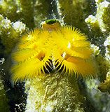
Split-plotIn an attempt to understand the effects on marine animals of short-term exposure to toxic substances, such as might occur following a spill, or a major increase in storm water flows, a it was decided to examine the toxicant in question, Copper, as part of a field experiment in Honk Kong. The experiment consisted of small sources of Cu (small, hemispherical plaster blocks, impregnated with copper), which released the metal into sea water over 4 or 5 days. The organism whose response to Cu was being measured was a small, polychaete worm, Hydroides, that attaches to hard surfaces in the sea, and is one of the first species to colonize any surface that is submerged. The biological questions focused on whether the timing of exposure to Cu affects the overall abundance of these worms. The time period of interest was the first or second week after a surface being available.
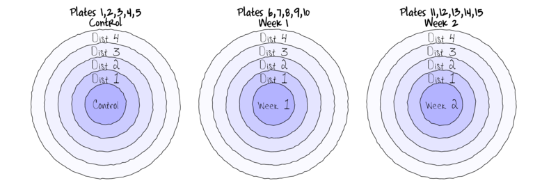
The experimental setup consisted of sheets of black perspex (settlement plates), which provided good surfaces for these worms. Each plate had a plaster block bolted to its centre, and the dissolving block would create a gradient of [Cu] across the plate. Over the two weeks of the experiment, a given plate would have pl ain plaster blocks (Control) or a block containing copper in the first week, followed by a plain block, or a plain block in the first week, followed by a dose of copper in the second week. After two weeks in the water, plates were removed and counted back in the laboratory. Without a clear idea of how sensitive these worms are to copper, an effect of the treatments might show up as an overall difference in the density of worms across a plate, or it could show up as a gradient in abundance across the plate, with a different gradient in different treatments. Therefore, on each plate, the density of worms (#/cm2) was recorded at each of four distances from the center of the plate.
Download Copper data set| Format of copper.csv data file | |||||||||||||||||
|---|---|---|---|---|---|---|---|---|---|---|---|---|---|---|---|---|---|
|
 |
copper <- read.table('../downloads/data/copper.csv', header=T, sep=',', strip.white=T)
head(copper)
   COPPER PLATE DIST WORMS
1 control   200    4 11.50
2 control   200    3 13.00
3 control   200    2 13.50
4 control   200    1 12.00
5 control    39    4 17.75
6 control    39    3 13.75
library(R2jags)
library(rstan)
library(coda)
The Plates are the "random" groups. Within each Plate, all levels of the Distance factor occur (this is a within group factor). Each Plate can only be of one of the three levels of the Copper treatment. This is therefore a within group (nested) factor. Traditionally, this mixture of nested and randomized block design would be called a partly nested or split-plot design.
In Bayesian (multilevel modeling) terms, this is a multi-level model with one hierarchical level the Plates means and another representing the Copper treatment means (based on the Plate means).
Exploratory data analysis has indicated that the response variable could be normalized via a forth-root transformation.
- Fit a model for Randomized Complete Block
- Effects parameterization - random intercepts model (JAGS)
number of lesionsi = βSite j(i) + εi where ε ∼ N(0,σ2)treating Distance as a factor
View full codemodelString= ## write the model to a text file (I suggest you alter the path to somewhere more relevant ## to your system!) writeLines(modelString,con="../downloads/BUGSscripts/ws9.9bQ2.1a.txt")
#sort the data set so that the copper treatments are in a more logical order
copper.sort <- copper[order(copper$COPPER),]
copper.sort$COPPER <- factor(copper.sort$COPPER, levels = c("control", "Week 1", "Week 2"))
copper.sort$PLATE <- factor(copper.sort$PLATE, levels=unique(copper.sort$PLATE))
cu <- with(copper.sort,COPPER[match(unique(PLATE),PLATE)])
cu <- factor(cu, levels=c("control", "Week 1", "Week 2"))
copper.list <- with(copper.sort,
                         list(worms=WORMS,
                           dist=as.numeric(DIST),
               plate=as.numeric(PLATE),
                           copper=factor(as.numeric(cu)),
               cu=as.numeric(COPPER),
                           nDist=length(levels(as.factor(DIST))),
                           nPlate=length(levels(as.factor(PLATE))),
                           nCopper=length(levels(cu)),
                           n=nrow(copper.sort)
                           )
                           )
params <- c("g0","gamma.copper",
                  "beta.plate",
          "beta.dist",
                  "beta.CopperDist",
                  "Copper.means","Dist.means","CopperDist.means",
                  "sd.Dist","sd.Copper","sd.Plate","sd.Resid","sd.CopperDist",
                  "sigma.res","sigma.plate","sigma.copper","sigma.dist","sigma.copperdist"
                  )
adaptSteps = 1000
burnInSteps = 2000
nChains = 3
numSavedSteps = 5000
thinSteps = 10
nIter = ceiling((numSavedSteps * thinSteps)/nChains)

library(R2jags)
##
copper.r2jags.a <- jags(data=copper.list,
                                 inits=NULL, # since there are three chains
          parameters.to.save=params,
          model.file="../downloads/BUGSscripts/ws9.9bQ2.1a.txt",
          n.chains=3,
          n.iter=nIter,
          n.burnin=burnInSteps,
      n.thin=thinSteps
          )
Compiling model graph
   Resolving undeclared variables
   Allocating nodes
   Graph Size: 458

Initializing model
print(copper.r2jags.a)
Inference for Bugs model at "../downloads/BUGSscripts/ws9.9bQ2.1a.txt", fit using jags, 3 chains, each with 16667 iterations (first 2000 discarded), n.thin = 10 n.sims = 4401 iterations saved mu.vect sd.vect 2.5% 25% 50% 75% 97.5% Rhat n.eff Copper.means[1] 10.861 0.700 9.484 10.400 10.865 11.324 12.218 1.001 4400 Copper.means[2] 6.950 0.681 5.577 6.503 6.955 7.412 8.274 1.002 1300 Copper.means[3] 0.505 0.679 -0.814 0.044 0.499 0.932 1.879 1.003 950 CopperDist.means[1,1] 10.861 0.700 9.484 10.400 10.865 11.324 12.218 1.001 4400 CopperDist.means[2,1] 6.950 0.681 5.577 6.503 6.955 7.412 8.274 1.002 1300 CopperDist.means[3,1] 0.505 0.679 -0.814 0.044 0.499 0.932 1.879 1.003 950 CopperDist.means[1,2] 11.998 0.679 10.629 11.525 12.022 12.460 13.254 1.001 4400 CopperDist.means[2,2] 8.400 0.675 7.079 7.957 8.391 8.837 9.736 1.001 4400 CopperDist.means[3,2] 1.570 0.695 0.242 1.113 1.558 2.028 2.985 1.001 4400 CopperDist.means[1,3] 12.437 0.622 11.171 12.034 12.459 12.840 13.643 1.001 4400 CopperDist.means[2,3] 8.592 0.685 7.232 8.145 8.597 9.050 9.912 1.001 4400 CopperDist.means[3,3] 3.956 0.679 2.612 3.498 3.955 4.392 5.307 1.001 3300 CopperDist.means[1,4] 13.502 0.713 12.117 13.032 13.493 13.969 14.918 1.001 4000 CopperDist.means[2,4] 10.075 0.670 8.766 9.634 10.077 10.515 11.419 1.001 4200 CopperDist.means[3,4] 7.549 0.721 6.113 7.080 7.564 8.032 8.936 1.001 4400 Dist.means[1] 6.111 0.361 5.428 5.865 6.106 6.350 6.857 1.001 4400 Dist.means[2] 7.248 0.786 5.667 6.739 7.271 7.770 8.792 1.001 4400 Dist.means[3] 7.687 0.747 6.211 7.201 7.680 8.168 9.159 1.001 4400 Dist.means[4] 8.752 0.820 7.178 8.192 8.748 9.289 10.409 1.001 4400 beta.CopperDist[1,1] 0.000 0.000 0.000 0.000 0.000 0.000 0.000 1.000 1 beta.CopperDist[2,1] 0.000 0.000 0.000 0.000 0.000 0.000 0.000 1.000 1 beta.CopperDist[3,1] 0.000 0.000 0.000 0.000 0.000 0.000 0.000 1.000 1 beta.CopperDist[1,2] 0.000 0.000 0.000 0.000 0.000 0.000 0.000 1.000 1 beta.CopperDist[2,2] 0.313 1.222 -2.093 -0.487 0.307 1.132 2.704 1.001 4400 beta.CopperDist[3,2] -0.073 1.172 -2.417 -0.855 -0.068 0.711 2.250 1.002 1400 beta.CopperDist[1,3] 0.000 0.000 0.000 0.000 0.000 0.000 0.000 1.000 1 beta.CopperDist[2,3] 0.067 1.182 -2.269 -0.740 0.064 0.869 2.391 1.001 4200 beta.CopperDist[3,3] 1.875 1.175 -0.530 1.109 1.912 2.653 4.163 1.002 1300 beta.CopperDist[1,4] 0.000 0.000 0.000 0.000 0.000 0.000 0.000 1.000 1 beta.CopperDist[2,4] 0.485 1.194 -1.873 -0.302 0.475 1.284 2.828 1.001 3300 beta.CopperDist[3,4] 4.403 1.306 1.780 3.541 4.419 5.300 6.858 1.001 3100 beta.dist[1] 0.000 0.000 0.000 0.000 0.000 0.000 0.000 1.000 1 beta.dist[2] 1.137 0.873 -0.629 0.579 1.150 1.721 2.812 1.001 4400 beta.dist[3] 1.576 0.836 -0.098 1.032 1.576 2.129 3.218 1.001 4400 beta.dist[4] 2.641 0.909 0.860 2.023 2.637 3.257 4.413 1.001 4400 beta.plate[1] 10.979 0.751 9.531 10.484 10.985 11.458 12.436 1.001 4400 beta.plate[2] 11.649 0.870 10.011 11.049 11.613 12.242 13.386 1.001 4400 beta.plate[3] 10.456 0.783 8.946 9.933 10.452 10.977 12.008 1.002 2000 beta.plate[4] 10.526 0.766 9.003 10.008 10.519 11.048 12.031 1.001 4400 beta.plate[5] 10.744 0.742 9.311 10.241 10.761 11.219 12.194 1.001 4400 beta.plate[6] 6.855 0.712 5.401 6.394 6.861 7.343 8.209 1.001 4000 beta.plate[7] 6.493 0.758 4.909 6.007 6.521 6.997 7.914 1.004 650 beta.plate[8] 7.240 0.740 5.772 6.726 7.234 7.735 8.730 1.001 3600 beta.plate[9] 7.099 0.727 5.673 6.597 7.095 7.596 8.495 1.004 920 beta.plate[10] 7.113 0.727 5.692 6.614 7.102 7.597 8.608 1.003 1200 beta.plate[11] 0.420 0.731 -1.008 -0.063 0.424 0.906 1.850 1.003 730 beta.plate[12] 0.366 0.732 -1.089 -0.107 0.360 0.840 1.846 1.002 2200 beta.plate[13] 0.374 0.729 -1.010 -0.129 0.367 0.875 1.777 1.002 1500 beta.plate[14] 0.710 0.734 -0.714 0.204 0.702 1.195 2.181 1.002 1700 beta.plate[15] 0.642 0.721 -0.763 0.152 0.640 1.104 2.070 1.003 770 g0 10.861 0.700 9.484 10.400 10.865 11.324 12.218 1.001 4400 gamma.copper[1] 0.000 0.000 0.000 0.000 0.000 0.000 0.000 1.000 1 gamma.copper[2] -3.912 0.974 -5.788 -4.560 -3.899 -3.290 -1.996 1.001 2800 gamma.copper[3] -10.356 0.962 -12.228 -11.004 -10.365 -9.711 -8.461 1.002 1500 sd.Copper 5.252 0.478 4.326 4.931 5.255 5.575 6.184 1.002 1400 sd.CopperDist 1.484 0.344 0.806 1.248 1.488 1.714 2.171 1.002 1500 sd.Dist 1.195 0.361 0.493 0.947 1.192 1.436 1.911 1.001 4400 sd.Plate 0.530 0.275 0.037 0.328 0.544 0.724 1.048 1.017 410 sd.Resid 4.304 0.000 4.304 4.304 4.304 4.304 4.304 1.000 1 sigma.copper 29.938 25.719 2.990 8.769 20.985 45.325 91.652 1.002 1300 sigma.copperdist 2.623 1.488 0.940 1.690 2.265 3.103 6.467 1.002 2000 sigma.dist 3.399 5.563 0.142 0.855 1.644 3.502 18.960 1.002 1800 sigma.plate 0.581 0.331 0.038 0.340 0.561 0.790 1.296 1.016 400 sigma.res 1.403 0.168 1.122 1.284 1.391 1.504 1.769 1.001 4400 deviance 208.941 8.827 193.172 202.427 208.707 214.673 226.700 1.001 4400 For each parameter, n.eff is a crude measure of effective sample size, and Rhat is the potential scale reduction factor (at convergence, Rhat=1). DIC info (using the rule, pD = var(deviance)/2) pD = 39.0 and DIC = 247.9 DIC is an estimate of expected predictive error (lower deviance is better). - Matrix parameterization - random intercepts model (JAGS)
number of lesionsi = βSite j(i) + εi where ε ∼ N(0,σ2)treating Distance as a factor
View full codeWe can perform generate the finite-population standard deviation posteriors within RmodelString=" model { #Likelihood for (i in 1:n) { y[i]~dnorm(mu[i],tau.res) mu[i] <- inprod(beta[],X[i,]) + inprod(gamma[],Z[i,]) y.err[i] <- y[i] - mu[1] } #Priors and derivatives for (i in 1:nZ) { gamma[i] ~ dnorm(0,tau.plate) } for (i in 1:nX) { beta[i] ~ dnorm(0,1.0E-06) } tau.res <- pow(sigma.res,-2) sigma.res <- z/sqrt(chSq) z ~ dnorm(0, .0016)I(0,) chSq ~ dgamma(0.5, 0.5) tau.plate <- pow(sigma.plate,-2) sigma.plate <- z.plate/sqrt(chSq.plate) z.plate ~ dnorm(0, .0016)I(0,) chSq.plate ~ dgamma(0.5, 0.5) } " ## write the model to a text file (I suggest you alter the path to somewhere more relevant ## to your system!) writeLines(modelString,con="../downloads/BUGSscripts/ws9.4bQ2.1b.txt") #sort the data set so that the copper treatments are in a more logical order library(dplyr) copper$DIST <- factor(copper$DIST) copper$PLATE <- factor(copper$PLATE) copper.sort <- arrange(copper,COPPER,PLATE,DIST) Xmat <- model.matrix(~COPPER*DIST, data=copper.sort) Zmat <- model.matrix(~-1+PLATE, data=copper.sort) copper.list <- list(y=copper.sort$WORMS, X=Xmat, nX=ncol(Xmat), Z=Zmat, nZ=ncol(Zmat), n=nrow(copper.sort) ) params <- c("beta","gamma", "sigma.res","sigma.plate") burnInSteps = 3000 nChains = 3 numSavedSteps = 3000 thinSteps = 100 nIter = ceiling((numSavedSteps * thinSteps)/nChains) library(R2jags) library(coda) ## copper.r2jags.b <- jags(data=copper.list, inits=NULL, # since there are three chains parameters.to.save=params, model.file="../downloads/BUGSscripts/ws9.4bQ2.1b.txt", n.chains=3, n.iter=nIter, n.burnin=burnInSteps, n.thin=thinSteps )
Compiling model graph
   Resolving undeclared variables
   Allocating nodes
   Graph Size: 1971

Initializing model
print(copper.r2jags.b)
Inference for Bugs model at "../downloads/BUGSscripts/ws9.4bQ2.1b.txt", fit using jags,
 3 chains, each with 1e+05 iterations (first 3000 discarded), n.thin = 100
 n.sims = 2910 iterations saved
            mu.vect sd.vect    2.5%     25%     50%     75%   97.5%  Rhat n.eff
beta[1]      10.846   0.692   9.516  10.383  10.838  11.308  12.181 1.001  2900
beta[2]      -3.601   0.985  -5.536  -4.261  -3.594  -2.942  -1.706 1.001  2900
beta[3]     -10.585   0.986 -12.566 -11.223 -10.576  -9.937  -8.681 1.001  2900
beta[4]       1.157   0.894  -0.638   0.559   1.140   1.770   2.866 1.001  2100
beta[5]       1.564   0.907  -0.215   0.958   1.568   2.165   3.374 1.001  2900
beta[6]       2.718   0.886   1.001   2.156   2.705   3.308   4.513 1.001  2900
beta[7]      -0.051   1.279  -2.460  -0.953  -0.053   0.802   2.504 1.001  2200
beta[8]       0.038   1.270  -2.333  -0.816   0.042   0.860   2.573 1.001  2900
beta[9]      -0.310   1.276  -2.806  -1.189  -0.295   0.534   2.177 1.001  2900
beta[10]      2.189   1.255  -0.281   1.353   2.210   3.025   4.629 1.001  2900
beta[11]      0.029   1.256  -2.408  -0.799   0.026   0.874   2.522 1.000  2900
beta[12]      4.870   1.248   2.432   4.031   4.879   5.668   7.329 1.001  2900
gamma[1]      0.148   0.492  -0.782  -0.119   0.083   0.406   1.257 1.001  2900
gamma[2]     -0.128   0.484  -1.186  -0.396  -0.081   0.140   0.814 1.001  2900
gamma[3]      0.293   0.525  -0.653  -0.031   0.210   0.581   1.490 1.001  2900
gamma[4]     -0.409   0.546  -1.637  -0.721  -0.312  -0.017   0.462 1.001  2900
gamma[5]     -0.357   0.525  -1.576  -0.664  -0.264   0.001   0.502 1.000  2900
gamma[6]      0.757   0.661  -0.176   0.224   0.682   1.152   2.271 1.002  1700
gamma[7]     -0.140   0.474  -1.165  -0.412  -0.074   0.117   0.770 1.001  2900
gamma[8]     -0.454   0.547  -1.682  -0.808  -0.374  -0.047   0.435 1.001  2900
gamma[9]      0.123   0.492  -0.824  -0.150   0.067   0.393   1.173 1.001  2900
gamma[10]    -0.102   0.500  -1.166  -0.369  -0.058   0.173   0.866 1.001  2900
gamma[11]    -0.130   0.466  -1.138  -0.391  -0.069   0.129   0.772 1.001  2200
gamma[12]     0.212   0.497  -0.689  -0.079   0.140   0.499   1.314 1.001  2900
gamma[13]     0.146   0.504  -0.843  -0.126   0.087   0.413   1.248 1.001  2100
gamma[14]     0.121   0.477  -0.806  -0.148   0.078   0.370   1.169 1.001  2400
gamma[15]    -0.089   0.472  -1.141  -0.340  -0.053   0.173   0.846 1.001  2900
sigma.plate   0.581   0.327   0.043   0.351   0.564   0.776   1.288 1.010  1700
sigma.res     1.401   0.168   1.116   1.281   1.391   1.505   1.769 1.002  1600
deviance    208.982   8.615 193.148 202.766 208.815 214.662 226.352 1.003   870

For each parameter, n.eff is a crude measure of effective sample size,
and Rhat is the potential scale reduction factor (at convergence, Rhat=1).

DIC info (using the rule, pD = var(deviance)/2)
pD = 37.0 and DIC = 246.0
DIC is an estimate of expected predictive error (lower deviance is better).
copper.mcmc.b <- as.mcmc(copper.r2jags.b$BUGSoutput$sims.matrix)
View full codecopper.sort <- arrange(copper,COPPER,PLATE,DIST) nms <- colnames(copper.mcmc.b) pred <- grep('beta|gamma',nms) coefs <- copper.mcmc.b[,pred] newdata <- copper.sort #unique(subset(copper, select=c('COPPER','DIST','PLATE'))) Amat <- cbind(model.matrix(~COPPER*DIST, newdata),model.matrix(~-1+PLATE, newdata)) pred <- coefs %*% t(Amat) y.err <- t(copper.sort$WORMS - t(pred)) a<-apply(y.err, 1,sd) resid.sd <- data.frame(Source='Resid',Median=median(a), HPDinterval(as.mcmc(a)), HPDinterval(as.mcmc(a), p=0.68)) ## Fixed effects nms <- colnames(copper.mcmc.b) copper.mcmc.b.beta <- copper.mcmc.b[,grep('beta',nms)] assign <- attr(Xmat, 'assign') nms <- attr(terms(model.frame(~COPPER*DIST, copper.sort)),'term.labels') fixed.sd <- NULL for (i in 1:max(assign)) { w <- which(i==assign) fixed.sd<-cbind(fixed.sd, apply(copper.mcmc.b.beta[,w],1,sd)) } library(plyr) fixed.sd <-adply(fixed.sd,2,function(x) { data.frame(Median=median(x), HPDinterval(as.mcmc(x)), HPDinterval(as.mcmc(x), p=0.68)) }) fixed.sd<- cbind(Source=nms, fixed.sd) # Variances nms <- colnames(copper.mcmc.b) copper.mcmc.b.gamma <- copper.mcmc.b[,grep('gamma',nms)] assign <- attr(Zmat, 'assign') nms <- attr(terms(model.frame(~-1+PLATE, copper.sort)),'term.labels') random.sd <- NULL for (i in 1:max(assign)) { w <- which(i==assign) random.sd<-cbind(random.sd, apply(copper.mcmc.b.gamma[,w],1,sd)) } library(plyr) random.sd <-adply(random.sd,2,function(x) { data.frame(Median=median(x), HPDinterval(as.mcmc(x)), HPDinterval(as.mcmc(x), p=0.68)) }) random.sd<- cbind(Source=nms, random.sd) (copper.sd <- rbind(subset(fixed.sd, select=-X1), subset(random.sd, select=-X1), resid.sd))
          Source Median     lower  upper lower.1 upper.1
1         COPPER 4.9456 3.555e+00 6.2986  4.2362  5.5965
2           DIST 0.9359 1.692e-01 1.6999  0.5042  1.2939
3    COPPER:DIST 2.2144 1.300e+00 3.0873  1.7050  2.6000
4          PLATE 0.5280 7.412e-05 0.9636  0.2703  0.8234
var1       Resid 1.3666 1.183e+00 1.5514  1.2620  1.4506
- Matrix parameterization - random intercepts model (STAN)
View full coderstanString=" data{ int n; int nZ; int nX; vector [n] y; matrix [n,nX] X; matrix [n,nZ] Z; vector [nX] a0; matrix [nX,nX] A0; } parameters{ vector [nX] beta; real<lower=0> sigma; vector [nZ] gamma; real<lower=0> sigma_Z; } transformed parameters { vector [n] mu; mu <- X*beta + Z*gamma; } model{ // Priors beta ~ multi_normal(a0,A0); gamma ~ normal( 0 , sigma_Z ); sigma_Z ~ cauchy(0,25); sigma ~ cauchy(0,25); y ~ normal( mu , sigma ); } generated quantities { vector [n] y_err; real<lower=0> sd_Resid; y_err <- y - mu; sd_Resid <- sd(y_err); } " #sort the data set so that the copper treatments are in a more logical order library(dplyr) copper$DIST <- factor(copper$DIST) copper$PLATE <- factor(copper$PLATE) copper.sort <- arrange(copper,COPPER,PLATE,DIST) Xmat <- model.matrix(~COPPER*DIST, data=copper.sort) Zmat <- model.matrix(~-1+PLATE, data=copper.sort) copper.list <- list(y=copper.sort$WORMS, X=Xmat, nX=ncol(Xmat), Z=Zmat, nZ=ncol(Zmat), n=nrow(copper.sort), a0=rep(0,ncol(Xmat)), A0=diag(100000,ncol(Xmat)) ) params <- c("beta","gamma", "sigma","sigma_Z") burnInSteps = 3000 nChains = 3 numSavedSteps = 3000 thinSteps = 100 nIter = ceiling((numSavedSteps * thinSteps)/nChains) library(rstan) library(coda) ## copper.rstan.a <- stan(data=copper.list, model_code=rstanString, pars=c("beta","gamma","sigma","sigma_Z"), chains=nChains, iter=nIter, warmup=burnInSteps, thin=thinSteps, save_dso=TRUE )
TRANSLATING MODEL 'rstanString' FROM Stan CODE TO C++ CODE NOW.
COMPILING THE C++ CODE FOR MODEL 'rstanString' NOW.

SAMPLING FOR MODEL 'rstanString' NOW (CHAIN 1).

Iteration:     1 / 100000 [  0%]  (Warmup)
Iteration:  3001 / 100000 [  3%]  (Sampling)
Iteration: 13000 / 100000 [ 13%]  (Sampling)
Iteration: 23000 / 100000 [ 23%]  (Sampling)
Iteration: 33000 / 100000 [ 33%]  (Sampling)
Iteration: 43000 / 100000 [ 43%]  (Sampling)
Iteration: 53000 / 100000 [ 53%]  (Sampling)
Iteration: 63000 / 100000 [ 63%]  (Sampling)
Iteration: 73000 / 100000 [ 73%]  (Sampling)
Iteration: 83000 / 100000 [ 83%]  (Sampling)
Iteration: 93000 / 100000 [ 93%]  (Sampling)
Iteration: 100000 / 100000 [100%]  (Sampling)
#  Elapsed Time: 1.83 seconds (Warm-up)
#                63.65 seconds (Sampling)
#                65.48 seconds (Total)


SAMPLING FOR MODEL 'rstanString' NOW (CHAIN 2).

Iteration:     1 / 100000 [  0%]  (Warmup)
Iteration:  3001 / 100000 [  3%]  (Sampling)
Iteration: 13000 / 100000 [ 13%]  (Sampling)
Iteration: 23000 / 100000 [ 23%]  (Sampling)
Iteration: 33000 / 100000 [ 33%]  (Sampling)
Iteration: 43000 / 100000 [ 43%]  (Sampling)
Iteration: 53000 / 100000 [ 53%]  (Sampling)
Iteration: 63000 / 100000 [ 63%]  (Sampling)
Iteration: 73000 / 100000 [ 73%]  (Sampling)
Iteration: 83000 / 100000 [ 83%]  (Sampling)
Iteration: 93000 / 100000 [ 93%]  (Sampling)
Iteration: 100000 / 100000 [100%]  (Sampling)
#  Elapsed Time: 1.77 seconds (Warm-up)
#                63.54 seconds (Sampling)
#                65.31 seconds (Total)


SAMPLING FOR MODEL 'rstanString' NOW (CHAIN 3).

Iteration:     1 / 100000 [  0%]  (Warmup)
Iteration:  3001 / 100000 [  3%]  (Sampling)
Iteration: 13000 / 100000 [ 13%]  (Sampling)
Iteration: 23000 / 100000 [ 23%]  (Sampling)
Iteration: 33000 / 100000 [ 33%]  (Sampling)
Iteration: 43000 / 100000 [ 43%]  (Sampling)
Iteration: 53000 / 100000 [ 53%]  (Sampling)
Iteration: 63000 / 100000 [ 63%]  (Sampling)
Iteration: 73000 / 100000 [ 73%]  (Sampling)
Iteration: 83000 / 100000 [ 83%]  (Sampling)
Iteration: 93000 / 100000 [ 93%]  (Sampling)
Iteration: 100000 / 100000 [100%]  (Sampling)
#  Elapsed Time: 1.86 seconds (Warm-up)
#                60.9 seconds (Sampling)
#                62.76 seconds (Total)
print(copper.rstan.a)
Inference for Stan model: rstanString.
3 chains, each with iter=1e+05; warmup=3000; thin=100;
post-warmup draws per chain=970, total post-warmup draws=2910.

            mean se_mean   sd   2.5%    25%    50%    75%  97.5% n_eff Rhat
beta[1]    10.85    0.01 0.70   9.49  10.36  10.85  11.32  12.18  2856    1
beta[2]    -3.60    0.02 0.97  -5.49  -4.25  -3.61  -2.95  -1.71  2910    1
beta[3]   -10.59    0.02 0.98 -12.51 -11.27 -10.60  -9.95  -8.61  2768    1
beta[4]     1.14    0.02 0.88  -0.62   0.57   1.15   1.74   2.83  2795    1
beta[5]     1.55    0.02 0.89  -0.27   0.97   1.55   2.16   3.30  2891    1
beta[6]     2.68    0.02 0.90   0.93   2.09   2.66   3.29   4.43  2910    1
beta[7]    -0.01    0.02 1.23  -2.40  -0.82  -0.03   0.78   2.48  2767    1
beta[8]     0.06    0.02 1.27  -2.48  -0.76   0.08   0.88   2.56  2808    1
beta[9]    -0.28    0.02 1.25  -2.75  -1.10  -0.29   0.53   2.18  2910    1
beta[10]    2.19    0.02 1.25  -0.27   1.34   2.19   3.01   4.69  2910    1
beta[11]    0.08    0.02 1.26  -2.37  -0.75   0.07   0.92   2.59  2698    1
beta[12]    4.91    0.02 1.26   2.37   4.06   4.94   5.76   7.36  2910    1
gamma[1]    0.16    0.01 0.50  -0.82  -0.13   0.10   0.43   1.26  2910    1
gamma[2]   -0.14    0.01 0.48  -1.16  -0.41  -0.11   0.13   0.83  2723    1
gamma[3]    0.27    0.01 0.52  -0.69  -0.04   0.21   0.55   1.47  2684    1
gamma[4]   -0.43    0.01 0.57  -1.72  -0.76  -0.33  -0.03   0.50  2910    1
gamma[5]   -0.36    0.01 0.52  -1.55  -0.67  -0.28  -0.01   0.57  2910    1
gamma[6]    0.80    0.01 0.67  -0.20   0.24   0.73   1.24   2.23  2910    1
gamma[7]   -0.15    0.01 0.50  -1.24  -0.43  -0.11   0.13   0.78  2910    1
gamma[8]   -0.50    0.01 0.57  -1.79  -0.86  -0.39  -0.08   0.38  2885    1
gamma[9]    0.15    0.01 0.49  -0.79  -0.13   0.09   0.42   1.23  2620    1
gamma[10]  -0.10    0.01 0.49  -1.17  -0.36  -0.06   0.18   0.84  2729    1
gamma[11]  -0.10    0.01 0.49  -1.14  -0.38  -0.07   0.15   0.89  2574    1
gamma[12]   0.23    0.01 0.51  -0.71  -0.07   0.16   0.50   1.35  2910    1
gamma[13]   0.14    0.01 0.49  -0.85  -0.15   0.09   0.40   1.24  2910    1
gamma[14]   0.12    0.01 0.49  -0.84  -0.17   0.07   0.38   1.24  2854    1
gamma[15]  -0.08    0.01 0.49  -1.17  -0.34  -0.05   0.20   0.90  2910    1
sigma       1.40    0.00 0.16   1.13   1.29   1.39   1.50   1.75  2910    1
sigma_Z     0.60    0.01 0.33   0.08   0.35   0.58   0.80   1.34  2690    1
lp__      -46.06    0.16 8.36 -60.39 -51.52 -47.16 -41.89 -24.81  2694    1

Samples were drawn using NUTS(diag_e) at Tue Mar 10 11:00:50 2015.
For each parameter, n_eff is a crude measure of effective sample size,
and Rhat is the potential scale reduction factor on split chains (at
convergence, Rhat=1).
copper.mcmc.c <- rstan:::as.mcmc.list.stanfit(copper.rstan.a) copper.mcmc.df.c <- as.data.frame(extract(copper.rstan.a))
- Effects parameterization - random intercepts model (JAGS)
- Before fully exploring the parameters, it is prudent to examine the convergence and mixing diagnostics.
Chose either any of the parameterizations (they should yield much the same) - although it is sometimes useful to explore the
different performances of effects vs matrix and JAGS vs STAN.
- Effects parameterization - random intercepts model (JAGS)
Full effects parameterization JAGS code
library(coda)
plot(as.mcmc(copper.r2jags.a))


autocorr.diag(as.mcmc(copper.r2jags.a))
beta.CopperDist[1,1] beta.CopperDist[1,2] beta.CopperDist[1,3] beta.CopperDist[1,4] Lag 0 NaN NaN NaN NaN Lag 10 NaN NaN NaN NaN Lag 50 NaN NaN NaN NaN Lag 100 NaN NaN NaN NaN Lag 500 NaN NaN NaN NaN beta.CopperDist[2,1] beta.CopperDist[2,2] beta.CopperDist[2,3] beta.CopperDist[2,4] Lag 0 NaN 1.00000 1.000000 1.000000 Lag 10 NaN 0.24469 0.222054 0.216291 Lag 50 NaN 0.05921 0.026555 0.045072 Lag 100 NaN -0.01081 -0.015542 -0.002378 Lag 500 NaN -0.00350 0.008972 -0.006634 beta.CopperDist[3,1] beta.CopperDist[3,2] beta.CopperDist[3,3] beta.CopperDist[3,4] Lag 0 NaN 1.000000 1.00000 1.00000 Lag 10 NaN 0.199025 0.23088 0.25306 Lag 50 NaN 0.022958 0.02120 0.05067 Lag 100 NaN 0.002325 -0.01310 0.02437 Lag 500 NaN -0.005242 0.01034 0.01639 beta.dist[1] beta.dist[2] beta.dist[3] beta.dist[4] beta.plate[1] beta.plate[10] Lag 0 NaN 1.000000 1.000000 1.00000 1.000000 1.00000 Lag 10 NaN 0.255021 0.251556 0.25802 0.287195 0.24511 Lag 50 NaN 0.044918 0.018411 0.05042 0.038350 0.03342 Lag 100 NaN 0.008341 0.009182 0.01449 0.004314 0.00491 Lag 500 NaN 0.004807 0.014703 0.00654 0.035690 -0.01577 beta.plate[11] beta.plate[12] beta.plate[13] beta.plate[14] beta.plate[15] beta.plate[2] Lag 0 1.00000 1.000000 1.000000 1.000000 1.000000 1.000000 Lag 10 0.25928 0.272842 0.264036 0.242892 0.258362 0.336103 Lag 50 0.06804 0.048872 0.047263 0.035472 0.025496 0.094944 Lag 100 0.02166 -0.007681 0.009033 0.016035 0.004158 0.006325 Lag 500 -0.02016 -0.006645 -0.008072 -0.003751 -0.034610 -0.002989 beta.plate[3] beta.plate[4] beta.plate[5] beta.plate[6] beta.plate[7] beta.plate[8] Lag 0 1.00000 1.00000 1.000000 1.00000 1.00000 1.00000 Lag 10 0.34339 0.33588 0.313348 0.23865 0.23797 0.27105 Lag 50 0.07035 0.07668 0.069223 0.02876 0.04548 0.04627 Lag 100 0.01688 0.01193 0.016767 -0.03244 -0.01375 0.01656 Lag 500 0.02176 0.02292 -0.007219 0.01029 -0.01057 -0.01247 beta.plate[9] CopperDist.means[1,1] CopperDist.means[1,2] CopperDist.means[1,3] Lag 0 1.0000000 1.00000 1.000000 1.000000 Lag 10 0.2226726 0.36190 0.054758 0.006662 Lag 50 0.0375715 0.06615 0.009547 -0.025679 Lag 100 -0.0016491 0.01054 0.001145 0.023196 Lag 500 -0.0008145 0.02561 0.019253 0.021300 CopperDist.means[1,4] CopperDist.means[2,1] CopperDist.means[2,2] CopperDist.means[2,3] Lag 0 1.00000 1.000000 1.00000 1.000000 Lag 10 0.05168 0.261546 0.01592 -0.026233 Lag 50 0.01046 0.053092 0.01705 -0.008165 Lag 100 0.01829 0.005019 -0.03090 -0.017731 Lag 500 0.01233 -0.008514 -0.01730 -0.011690 CopperDist.means[2,4] CopperDist.means[3,1] CopperDist.means[3,2] CopperDist.means[3,3] Lag 0 1.0000000 1.00000 1.000000 1.000000 Lag 10 -0.0165542 0.30018 0.008994 0.001836 Lag 50 -0.0192582 0.06384 0.009835 0.003129 Lag 100 0.0002611 0.01065 -0.029655 -0.002372 Lag 500 -0.0075805 -0.01479 -0.005899 -0.014576 CopperDist.means[3,4] Copper.means[1] Copper.means[2] Copper.means[3] deviance Lag 0 1.000000 1.00000 1.000000 1.00000 1.00000 Lag 10 0.006198 0.36190 0.261546 0.30018 0.20985 Lag 50 0.007538 0.06615 0.053092 0.06384 0.05707 Lag 100 -0.020224 0.01054 0.005019 0.01065 0.02854 Lag 500 0.013913 0.02561 -0.008514 -0.01479 0.03227 Dist.means[1] Dist.means[2] Dist.means[3] Dist.means[4] g0 gamma.copper[1] Lag 0 1.000000 1.000000 1.0000000 1.0000000 1.00000 NaN Lag 10 0.333067 0.218816 0.2107202 0.2127891 0.36190 NaN Lag 50 0.049868 0.044068 0.0125067 0.0357464 0.06615 NaN Lag 100 0.014842 -0.001023 -0.0003989 0.0197903 0.01054 NaN Lag 500 -0.005594 -0.003517 0.0058489 0.0007837 0.02561 NaN gamma.copper[2] gamma.copper[3] sd.Copper sd.CopperDist sd.Dist sd.Plate sd.Resid Lag 0 1.000000 1.000000 1.000000 1.000000 1.00000 1.00000 1.0000 Lag 10 0.337415 0.344864 0.338827 0.230669 0.22697 0.52631 0.1796 Lag 50 0.083646 0.051246 0.048962 0.041647 0.02992 0.14443 0.1798 Lag 100 0.008024 -0.003719 -0.003448 0.008505 0.01112 0.03803 0.1878 Lag 500 -0.003768 -0.003025 -0.001491 0.021038 0.01211 0.03867 0.1702 sigma.copper sigma.copperdist sigma.dist sigma.plate sigma.res Lag 0 1.000000 1.0000000 1.000000 1.00000 1.000000 Lag 10 0.124627 0.1642414 0.672842 0.49582 0.076779 Lag 50 0.037826 -0.0005846 0.195812 0.12442 0.030415 Lag 100 -0.005765 0.0167087 0.040776 0.02555 0.002363 Lag 500 0.018852 0.0147139 -0.009728 0.03517 0.014518raftery.diag(as.mcmc(copper.r2jags.a))
[[1]]

Quantile (q) = 0.025
Accuracy (r) = +/- 0.005
Probability (s) = 0.95

You need a sample size of at least 3746 with these values of q, r and s

[[2]]

Quantile (q) = 0.025
Accuracy (r) = +/- 0.005
Probability (s) = 0.95

You need a sample size of at least 3746 with these values of q, r and s

[[3]]

Quantile (q) = 0.025
Accuracy (r) = +/- 0.005
Probability (s) = 0.95

You need a sample size of at least 3746 with these values of q, r and s
- Matrix parameterization - random intercepts model (JAGS)
Matrix parameterization JAGS code
library(coda)
plot(as.mcmc(copper.r2jags.b))


autocorr.diag(as.mcmc(copper.r2jags.b))
beta[1] beta[10] beta[11] beta[12] beta[2] beta[3] beta[4] beta[5] Lag 0 1.0000000 1.000000 1.000000 1.000000 1.0000000 1.000000 1.000000 1.000000 Lag 100 0.0001407 -0.036177 -0.023323 -0.021760 -0.0162229 -0.005007 0.009196 0.011262 Lag 500 -0.0059944 0.008549 -0.048529 -0.001494 -0.0063997 -0.002699 -0.024990 -0.010342 Lag 1000 0.0337110 -0.005433 -0.003782 -0.005551 0.0001471 0.031625 0.019803 0.022166 Lag 5000 0.0049328 0.008552 0.020436 0.007391 -0.0170351 0.023017 -0.002698 -0.001328 beta[6] beta[7] beta[8] beta[9] deviance gamma[1] gamma[10] gamma[11] gamma[12] Lag 0 1.000000 1.000000 1.000000 1.000000 1.000000 1.000000 1.0000000 1.000000 1.00000 Lag 100 -0.025094 0.008480 0.006466 -0.003224 0.038513 0.018925 0.0056235 0.026267 -0.02103 Lag 500 -0.020629 -0.017689 -0.011594 -0.007384 -0.009974 -0.011192 -0.0170085 0.004762 -0.03566 Lag 1000 0.006279 0.012829 0.006970 0.011652 -0.042482 0.020043 0.0014589 0.012485 0.02791 Lag 5000 0.017429 -0.001059 0.034788 -0.013313 -0.014041 -0.007018 -0.0008621 -0.008544 -0.04511 gamma[13] gamma[14] gamma[15] gamma[2] gamma[3] gamma[4] gamma[5] gamma[6] gamma[7] Lag 0 1.000000 1.000000 1.00000 1.000000 1.00000 1.00000 1.00000 1.000000 1.000000 Lag 100 0.013589 0.034522 0.02127 0.014172 0.01249 0.03639 0.02257 0.084937 -0.008609 Lag 500 -0.004070 -0.006861 -0.02694 0.025126 0.03462 0.03974 0.00122 -0.006529 -0.013682 Lag 1000 -0.006163 -0.006785 0.01743 0.025884 0.01833 -0.02431 0.01137 -0.020079 -0.020895 Lag 5000 0.008686 -0.008047 -0.02145 -0.006345 -0.01477 0.02336 0.01776 -0.018813 0.001560 gamma[8] gamma[9] sigma.plate sigma.res Lag 0 1.000000 1.000000 1.000000 1.00000 Lag 100 0.005905 -0.014622 0.104277 0.04746 Lag 500 -0.031612 0.003044 0.006673 -0.02409 Lag 1000 -0.023723 -0.017751 -0.010621 -0.01146 Lag 5000 0.029605 0.025012 0.044462 -0.00495raftery.diag(as.mcmc(copper.r2jags.b))
[[1]]

Quantile (q) = 0.025
Accuracy (r) = +/- 0.005
Probability (s) = 0.95

You need a sample size of at least 3746 with these values of q, r and s

[[2]]

Quantile (q) = 0.025
Accuracy (r) = +/- 0.005
Probability (s) = 0.95

You need a sample size of at least 3746 with these values of q, r and s

[[3]]

Quantile (q) = 0.025
Accuracy (r) = +/- 0.005
Probability (s) = 0.95

You need a sample size of at least 3746 with these values of q, r and s
- Matrix parameterization - random intercepts model (STAN)
Matrix parameterization STAN code
library(coda)
plot(copper.mcmc.c)


autocorr.diag(copper.mcmc.c)
beta[1] beta[2] beta[3] beta[4] beta[5] beta[6] beta[7] beta[8] beta[9] Lag 0 1.000000 1.000000 1.000000 1.000000 1.000000 1.000000 1.0000000 1.00000 1.0000000 Lag 100 0.009967 -0.004816 0.026420 0.021262 0.004017 -0.011575 0.0258546 0.01863 -0.0191944 Lag 500 -0.026817 -0.015666 0.008346 -0.011776 -0.025410 -0.044671 0.0181025 -0.01384 -0.0240211 Lag 1000 -0.016257 -0.007606 -0.003394 -0.005554 -0.002241 -0.011314 -0.0001529 -0.01658 0.0003652 Lag 5000 0.024858 0.015632 0.014281 -0.006247 0.025912 -0.007806 -0.0110499 -0.01254 0.0420761 beta[10] beta[11] beta[12] gamma[1] gamma[2] gamma[3] gamma[4] gamma[5] Lag 0 1.0000000 1.000000 1.000000 1.0000000 1.000000 1.00000 1.000000 1.0000000 Lag 100 -0.0092496 0.009893 0.001023 -0.0286308 0.034164 0.01774 -0.017220 -0.0007568 Lag 500 -0.0003694 -0.036469 -0.046402 -0.0079941 -0.009406 -0.00739 0.015283 -0.0326711 Lag 1000 -0.0167486 0.005390 -0.027099 0.0032897 0.023751 -0.03079 -0.011388 -0.0104777 Lag 5000 0.0118440 -0.002303 0.006366 0.0008928 -0.029389 -0.05205 -0.006255 0.0056763 gamma[6] gamma[7] gamma[8] gamma[9] gamma[10] gamma[11] gamma[12] gamma[13] gamma[14] Lag 0 1.000000 1.0000000 1.000000 1.000000 1.000000 1.000000 1.000000 1.000000 1.00000 Lag 100 -0.003538 -0.0002712 0.004690 0.055281 0.008450 0.041792 -0.007299 -0.023793 0.01093 Lag 500 -0.014107 0.0109865 0.005891 0.011806 -0.005971 -0.006931 0.013032 0.006489 0.02300 Lag 1000 -0.011771 -0.0057208 -0.001124 0.018194 -0.014500 -0.006475 0.023547 0.007998 0.01502 Lag 5000 -0.010106 0.0258887 -0.015260 0.004726 -0.040014 -0.007669 0.002687 -0.022278 0.01922 gamma[15] sigma sigma_Z lp__ Lag 0 1.00000 1.000e+00 1.000000 1.000000 Lag 100 -0.03304 -1.168e-02 0.008867 0.041334 Lag 500 0.01004 2.075e-02 -0.002091 -0.020622 Lag 1000 0.01796 -5.713e-05 -0.001457 -0.005787 Lag 5000 0.01208 1.884e-02 -0.011151 -0.021067raftery.diag(copper.mcmc.c)
[[1]]

Quantile (q) = 0.025
Accuracy (r) = +/- 0.005
Probability (s) = 0.95

You need a sample size of at least 3746 with these values of q, r and s

[[2]]

Quantile (q) = 0.025
Accuracy (r) = +/- 0.005
Probability (s) = 0.95

You need a sample size of at least 3746 with these values of q, r and s

[[3]]

Quantile (q) = 0.025
Accuracy (r) = +/- 0.005
Probability (s) = 0.95

You need a sample size of at least 3746 with these values of q, r and s
- Effects parameterization - random intercepts model (JAGS)
- Explore the parameter estimates
Full effects parameterization JAGS code
library(R2jags)
print(copper.r2jags.a)
Inference for Bugs model at "../downloads/BUGSscripts/ws9.9bQ2.1a.txt", fit using jags,
 3 chains, each with 16667 iterations (first 2000 discarded), n.thin = 10
 n.sims = 4401 iterations saved
                      mu.vect sd.vect    2.5%     25%     50%     75%   97.5%  Rhat n.eff
Copper.means[1]        10.861   0.700   9.484  10.400  10.865  11.324  12.218 1.001  4400
Copper.means[2]         6.950   0.681   5.577   6.503   6.955   7.412   8.274 1.002  1300
Copper.means[3]         0.505   0.679  -0.814   0.044   0.499   0.932   1.879 1.003   950
CopperDist.means[1,1]  10.861   0.700   9.484  10.400  10.865  11.324  12.218 1.001  4400
CopperDist.means[2,1]   6.950   0.681   5.577   6.503   6.955   7.412   8.274 1.002  1300
CopperDist.means[3,1]   0.505   0.679  -0.814   0.044   0.499   0.932   1.879 1.003   950
CopperDist.means[1,2]  11.998   0.679  10.629  11.525  12.022  12.460  13.254 1.001  4400
CopperDist.means[2,2]   8.400   0.675   7.079   7.957   8.391   8.837   9.736 1.001  4400
CopperDist.means[3,2]   1.570   0.695   0.242   1.113   1.558   2.028   2.985 1.001  4400
CopperDist.means[1,3]  12.437   0.622  11.171  12.034  12.459  12.840  13.643 1.001  4400
CopperDist.means[2,3]   8.592   0.685   7.232   8.145   8.597   9.050   9.912 1.001  4400
CopperDist.means[3,3]   3.956   0.679   2.612   3.498   3.955   4.392   5.307 1.001  3300
CopperDist.means[1,4]  13.502   0.713  12.117  13.032  13.493  13.969  14.918 1.001  4000
CopperDist.means[2,4]  10.075   0.670   8.766   9.634  10.077  10.515  11.419 1.001  4200
CopperDist.means[3,4]   7.549   0.721   6.113   7.080   7.564   8.032   8.936 1.001  4400
Dist.means[1]           6.111   0.361   5.428   5.865   6.106   6.350   6.857 1.001  4400
Dist.means[2]           7.248   0.786   5.667   6.739   7.271   7.770   8.792 1.001  4400
Dist.means[3]           7.687   0.747   6.211   7.201   7.680   8.168   9.159 1.001  4400
Dist.means[4]           8.752   0.820   7.178   8.192   8.748   9.289  10.409 1.001  4400
beta.CopperDist[1,1]    0.000   0.000   0.000   0.000   0.000   0.000   0.000 1.000     1
beta.CopperDist[2,1]    0.000   0.000   0.000   0.000   0.000   0.000   0.000 1.000     1
beta.CopperDist[3,1]    0.000   0.000   0.000   0.000   0.000   0.000   0.000 1.000     1
beta.CopperDist[1,2]    0.000   0.000   0.000   0.000   0.000   0.000   0.000 1.000     1
beta.CopperDist[2,2]    0.313   1.222  -2.093  -0.487   0.307   1.132   2.704 1.001  4400
beta.CopperDist[3,2]   -0.073   1.172  -2.417  -0.855  -0.068   0.711   2.250 1.002  1400
beta.CopperDist[1,3]    0.000   0.000   0.000   0.000   0.000   0.000   0.000 1.000     1
beta.CopperDist[2,3]    0.067   1.182  -2.269  -0.740   0.064   0.869   2.391 1.001  4200
beta.CopperDist[3,3]    1.875   1.175  -0.530   1.109   1.912   2.653   4.163 1.002  1300
beta.CopperDist[1,4]    0.000   0.000   0.000   0.000   0.000   0.000   0.000 1.000     1
beta.CopperDist[2,4]    0.485   1.194  -1.873  -0.302   0.475   1.284   2.828 1.001  3300
beta.CopperDist[3,4]    4.403   1.306   1.780   3.541   4.419   5.300   6.858 1.001  3100
beta.dist[1]            0.000   0.000   0.000   0.000   0.000   0.000   0.000 1.000     1
beta.dist[2]            1.137   0.873  -0.629   0.579   1.150   1.721   2.812 1.001  4400
beta.dist[3]            1.576   0.836  -0.098   1.032   1.576   2.129   3.218 1.001  4400
beta.dist[4]            2.641   0.909   0.860   2.023   2.637   3.257   4.413 1.001  4400
beta.plate[1]          10.979   0.751   9.531  10.484  10.985  11.458  12.436 1.001  4400
beta.plate[2]          11.649   0.870  10.011  11.049  11.613  12.242  13.386 1.001  4400
beta.plate[3]          10.456   0.783   8.946   9.933  10.452  10.977  12.008 1.002  2000
beta.plate[4]          10.526   0.766   9.003  10.008  10.519  11.048  12.031 1.001  4400
beta.plate[5]          10.744   0.742   9.311  10.241  10.761  11.219  12.194 1.001  4400
beta.plate[6]           6.855   0.712   5.401   6.394   6.861   7.343   8.209 1.001  4000
beta.plate[7]           6.493   0.758   4.909   6.007   6.521   6.997   7.914 1.004   650
beta.plate[8]           7.240   0.740   5.772   6.726   7.234   7.735   8.730 1.001  3600
beta.plate[9]           7.099   0.727   5.673   6.597   7.095   7.596   8.495 1.004   920
beta.plate[10]          7.113   0.727   5.692   6.614   7.102   7.597   8.608 1.003  1200
beta.plate[11]          0.420   0.731  -1.008  -0.063   0.424   0.906   1.850 1.003   730
beta.plate[12]          0.366   0.732  -1.089  -0.107   0.360   0.840   1.846 1.002  2200
beta.plate[13]          0.374   0.729  -1.010  -0.129   0.367   0.875   1.777 1.002  1500
beta.plate[14]          0.710   0.734  -0.714   0.204   0.702   1.195   2.181 1.002  1700
beta.plate[15]          0.642   0.721  -0.763   0.152   0.640   1.104   2.070 1.003   770
g0                     10.861   0.700   9.484  10.400  10.865  11.324  12.218 1.001  4400
gamma.copper[1]         0.000   0.000   0.000   0.000   0.000   0.000   0.000 1.000     1
gamma.copper[2]        -3.912   0.974  -5.788  -4.560  -3.899  -3.290  -1.996 1.001  2800
gamma.copper[3]       -10.356   0.962 -12.228 -11.004 -10.365  -9.711  -8.461 1.002  1500
sd.Copper               5.252   0.478   4.326   4.931   5.255   5.575   6.184 1.002  1400
sd.CopperDist           1.484   0.344   0.806   1.248   1.488   1.714   2.171 1.002  1500
sd.Dist                 1.195   0.361   0.493   0.947   1.192   1.436   1.911 1.001  4400
sd.Plate                0.530   0.275   0.037   0.328   0.544   0.724   1.048 1.017   410
sd.Resid                4.304   0.000   4.304   4.304   4.304   4.304   4.304 1.000     1
sigma.copper           29.938  25.719   2.990   8.769  20.985  45.325  91.652 1.002  1300
sigma.copperdist        2.623   1.488   0.940   1.690   2.265   3.103   6.467 1.002  2000
sigma.dist              3.399   5.563   0.142   0.855   1.644   3.502  18.960 1.002  1800
sigma.plate             0.581   0.331   0.038   0.340   0.561   0.790   1.296 1.016   400
sigma.res               1.403   0.168   1.122   1.284   1.391   1.504   1.769 1.001  4400
deviance              208.941   8.827 193.172 202.427 208.707 214.673 226.700 1.001  4400

For each parameter, n.eff is a crude measure of effective sample size,
and Rhat is the potential scale reduction factor (at convergence, Rhat=1).

DIC info (using the rule, pD = var(deviance)/2)
pD = 39.0 and DIC = 247.9
DIC is an estimate of expected predictive error (lower deviance is better).
Matrix parameterization JAGS codelibrary(R2jags) print(copper.r2jags.b)
Inference for Bugs model at "../downloads/BUGSscripts/ws9.4bQ2.1b.txt", fit using jags,
 3 chains, each with 1e+05 iterations (first 3000 discarded), n.thin = 100
 n.sims = 2910 iterations saved
            mu.vect sd.vect    2.5%     25%     50%     75%   97.5%  Rhat n.eff
beta[1]      10.846   0.692   9.516  10.383  10.838  11.308  12.181 1.001  2900
beta[2]      -3.601   0.985  -5.536  -4.261  -3.594  -2.942  -1.706 1.001  2900
beta[3]     -10.585   0.986 -12.566 -11.223 -10.576  -9.937  -8.681 1.001  2900
beta[4]       1.157   0.894  -0.638   0.559   1.140   1.770   2.866 1.001  2100
beta[5]       1.564   0.907  -0.215   0.958   1.568   2.165   3.374 1.001  2900
beta[6]       2.718   0.886   1.001   2.156   2.705   3.308   4.513 1.001  2900
beta[7]      -0.051   1.279  -2.460  -0.953  -0.053   0.802   2.504 1.001  2200
beta[8]       0.038   1.270  -2.333  -0.816   0.042   0.860   2.573 1.001  2900
beta[9]      -0.310   1.276  -2.806  -1.189  -0.295   0.534   2.177 1.001  2900
beta[10]      2.189   1.255  -0.281   1.353   2.210   3.025   4.629 1.001  2900
beta[11]      0.029   1.256  -2.408  -0.799   0.026   0.874   2.522 1.000  2900
beta[12]      4.870   1.248   2.432   4.031   4.879   5.668   7.329 1.001  2900
gamma[1]      0.148   0.492  -0.782  -0.119   0.083   0.406   1.257 1.001  2900
gamma[2]     -0.128   0.484  -1.186  -0.396  -0.081   0.140   0.814 1.001  2900
gamma[3]      0.293   0.525  -0.653  -0.031   0.210   0.581   1.490 1.001  2900
gamma[4]     -0.409   0.546  -1.637  -0.721  -0.312  -0.017   0.462 1.001  2900
gamma[5]     -0.357   0.525  -1.576  -0.664  -0.264   0.001   0.502 1.000  2900
gamma[6]      0.757   0.661  -0.176   0.224   0.682   1.152   2.271 1.002  1700
gamma[7]     -0.140   0.474  -1.165  -0.412  -0.074   0.117   0.770 1.001  2900
gamma[8]     -0.454   0.547  -1.682  -0.808  -0.374  -0.047   0.435 1.001  2900
gamma[9]      0.123   0.492  -0.824  -0.150   0.067   0.393   1.173 1.001  2900
gamma[10]    -0.102   0.500  -1.166  -0.369  -0.058   0.173   0.866 1.001  2900
gamma[11]    -0.130   0.466  -1.138  -0.391  -0.069   0.129   0.772 1.001  2200
gamma[12]     0.212   0.497  -0.689  -0.079   0.140   0.499   1.314 1.001  2900
gamma[13]     0.146   0.504  -0.843  -0.126   0.087   0.413   1.248 1.001  2100
gamma[14]     0.121   0.477  -0.806  -0.148   0.078   0.370   1.169 1.001  2400
gamma[15]    -0.089   0.472  -1.141  -0.340  -0.053   0.173   0.846 1.001  2900
sigma.plate   0.581   0.327   0.043   0.351   0.564   0.776   1.288 1.010  1700
sigma.res     1.401   0.168   1.116   1.281   1.391   1.505   1.769 1.002  1600
deviance    208.982   8.615 193.148 202.766 208.815 214.662 226.352 1.003   870

For each parameter, n.eff is a crude measure of effective sample size,
and Rhat is the potential scale reduction factor (at convergence, Rhat=1).

DIC info (using the rule, pD = var(deviance)/2)
pD = 37.0 and DIC = 246.0
DIC is an estimate of expected predictive error (lower deviance is better).
Matrix parameterization STAN codelibrary(R2jags) print(copper.rstan.a)
Inference for Stan model: rstanString. 3 chains, each with iter=1e+05; warmup=3000; thin=100; post-warmup draws per chain=970, total post-warmup draws=2910. mean se_mean sd 2.5% 25% 50% 75% 97.5% n_eff Rhat beta[1] 10.85 0.01 0.70 9.49 10.36 10.85 11.32 12.18 2856 1 beta[2] -3.60 0.02 0.97 -5.49 -4.25 -3.61 -2.95 -1.71 2910 1 beta[3] -10.59 0.02 0.98 -12.51 -11.27 -10.60 -9.95 -8.61 2768 1 beta[4] 1.14 0.02 0.88 -0.62 0.57 1.15 1.74 2.83 2795 1 beta[5] 1.55 0.02 0.89 -0.27 0.97 1.55 2.16 3.30 2891 1 beta[6] 2.68 0.02 0.90 0.93 2.09 2.66 3.29 4.43 2910 1 beta[7] -0.01 0.02 1.23 -2.40 -0.82 -0.03 0.78 2.48 2767 1 beta[8] 0.06 0.02 1.27 -2.48 -0.76 0.08 0.88 2.56 2808 1 beta[9] -0.28 0.02 1.25 -2.75 -1.10 -0.29 0.53 2.18 2910 1 beta[10] 2.19 0.02 1.25 -0.27 1.34 2.19 3.01 4.69 2910 1 beta[11] 0.08 0.02 1.26 -2.37 -0.75 0.07 0.92 2.59 2698 1 beta[12] 4.91 0.02 1.26 2.37 4.06 4.94 5.76 7.36 2910 1 gamma[1] 0.16 0.01 0.50 -0.82 -0.13 0.10 0.43 1.26 2910 1 gamma[2] -0.14 0.01 0.48 -1.16 -0.41 -0.11 0.13 0.83 2723 1 gamma[3] 0.27 0.01 0.52 -0.69 -0.04 0.21 0.55 1.47 2684 1 gamma[4] -0.43 0.01 0.57 -1.72 -0.76 -0.33 -0.03 0.50 2910 1 gamma[5] -0.36 0.01 0.52 -1.55 -0.67 -0.28 -0.01 0.57 2910 1 gamma[6] 0.80 0.01 0.67 -0.20 0.24 0.73 1.24 2.23 2910 1 gamma[7] -0.15 0.01 0.50 -1.24 -0.43 -0.11 0.13 0.78 2910 1 gamma[8] -0.50 0.01 0.57 -1.79 -0.86 -0.39 -0.08 0.38 2885 1 gamma[9] 0.15 0.01 0.49 -0.79 -0.13 0.09 0.42 1.23 2620 1 gamma[10] -0.10 0.01 0.49 -1.17 -0.36 -0.06 0.18 0.84 2729 1 gamma[11] -0.10 0.01 0.49 -1.14 -0.38 -0.07 0.15 0.89 2574 1 gamma[12] 0.23 0.01 0.51 -0.71 -0.07 0.16 0.50 1.35 2910 1 gamma[13] 0.14 0.01 0.49 -0.85 -0.15 0.09 0.40 1.24 2910 1 gamma[14] 0.12 0.01 0.49 -0.84 -0.17 0.07 0.38 1.24 2854 1 gamma[15] -0.08 0.01 0.49 -1.17 -0.34 -0.05 0.20 0.90 2910 1 sigma 1.40 0.00 0.16 1.13 1.29 1.39 1.50 1.75 2910 1 sigma_Z 0.60 0.01 0.33 0.08 0.35 0.58 0.80 1.34 2690 1 lp__ -46.06 0.16 8.36 -60.39 -51.52 -47.16 -41.89 -24.81 2694 1 Samples were drawn using NUTS(diag_e) at Tue Mar 10 11:00:50 2015. For each parameter, n_eff is a crude measure of effective sample size, and Rhat is the potential scale reduction factor on split chains (at convergence, Rhat=1). - Figure time
Matrix parameterization JAGS code
nms <- colnames(copper.mcmc.b)
pred <- grep('beta',nms)
coefs <- copper.mcmc.b[,pred]
newdata <- expand.grid(COPPER=levels(copper$COPPER), DIST=levels(copper$DIST))
Xmat <- model.matrix(~COPPER*DIST, newdata)
pred <- coefs %*% t(Xmat)
library(plyr)
newdata <- cbind(newdata, adply(pred, 2, function(x) {
   data.frame(Median=median(x), HPDinterval(as.mcmc(x)), HPDinterval(as.mcmc(x), p=0.68))
}))
newdata
    COPPER DIST X1  Median   lower  upper lower.1 upper.1
1  control    1  1 10.8380  9.5248 12.186 10.2017 11.5612
2   Week 1    1  2  7.2451  5.8848  8.574  6.6030  7.9287
3   Week 2    1  3  0.2601 -1.0866  1.668 -0.3530  0.9995
4  control    2  4 11.9839 10.6367 13.262 11.2598 12.6376
5   Week 1    2  5  8.3606  6.9853  9.650  7.6200  9.0231
6   Week 2    2  6  1.4546  0.1709  2.884  0.8285  2.1123
7  control    3  7 12.4044 11.0236 13.735 11.6569 13.0335
8   Week 1    3  8  8.5025  7.2147  9.969  7.7567  9.1611
9   Week 2    3  9  4.0181  2.6460  5.388  3.2516  4.6498
10 control    4 10 13.5746 12.1840 14.933 12.9667 14.2964
11  Week 1    4 11  9.9770  8.7576 11.452  9.2903 10.6905
12  Week 2    4 12  7.8511  6.4945  9.192  7.1457  8.5044
library(ggplot2)
p1 <-ggplot(newdata, aes(y=Median, x=as.integer(DIST), fill=COPPER)) +
  geom_line(aes(linetype=COPPER)) +
  #geom_line()+
  geom_linerange(aes(ymin=lower, ymax=upper), show_guide=FALSE)+
  geom_linerange(aes(ymin=lower.1, ymax=upper.1), size=2,show_guide=FALSE)+
  geom_point(size=3, shape=21)+
  scale_y_continuous(expression(Density~of~worms~(cm^2)))+
  scale_x_continuous('Distance from plate center')+
  scale_fill_manual('Treatment', breaks=c('control','Week 1', 'Week 2'), values=c('black','white','grey'),
                    labels=c('Control','Week 1','Week 2'))+
  scale_linetype_manual('Treatment', breaks=c('control','Week 1', 'Week 2'), values=c('solid','dashed','dotted'),
                    labels=c('Control','Week 1','Week 2'))+
  theme_classic() +
  theme(legend.justification=c(1,0), legend.position=c(1,0),
        legend.key.width=unit(3,'lines'),
        axis.title.y=element_text(vjust=2, size=rel(1.2)),
        axis.title.x=element_text(vjust=-1, size=rel(1.2)),
        plot.margin=unit(c(0.5,0.5,1,2),'lines'))

copper.sd$Source <- factor(copper.sd$Source, levels=c("Resid","COPPER:DIST","DIST","PLATE","COPPER"),
    labels=c("Residuals", "Copper:Dist", "Dist","Plates","Copper"))
copper.sd$Perc <- 100*copper.sd$Median/sum(copper.sd$Median)

p2<-ggplot(copper.sd,aes(y=Source, x=Median))+
  geom_vline(xintercept=0,linetype="dashed")+
  geom_hline(xintercept=0)+
  scale_x_continuous("Finite population \nvariance components (sd)")+
  geom_errorbarh(aes(xmin=lower.1, xmax=upper.1), height=0, size=1)+
  geom_errorbarh(aes(xmin=lower, xmax=upper), height=0, size=1.5)+
  geom_point(size=3)+
  geom_text(aes(label=sprintf("(%4.1f%%)",Perc),vjust=-1))+
  theme_classic()+
  theme(axis.line=element_blank(),axis.title.y=element_blank(),
       axis.text.y=element_text(size=12,hjust=1))

library(gridExtra)
grid.arrange(p1, p2, ncol=2)

Repeated Measures
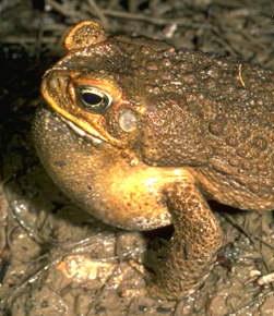
Repeated MeasuresIn an honours thesis from (1992), Mullens was investigating the ways that cane toads ( Bufo marinus ) respond to conditions of hypoxia. Toads show two different kinds of breathing patterns, lung or buccal, requiring them to be treated separately in the experiment. Her aim was to expose toads to a range of O2 concentrations, and record their breathing patterns, including parameters such as the expired volume for individual breaths. It was desirable to have around 8 replicates to compare the responses of the two breathing types, and the complication is that animals are expensive, and different individuals are likely to have different O2 profiles (leading to possibly reduced power). There are two main design options for this experiment;
- One animal per O2 treatment, 8 concentrations, 2 breathing types. With 8 replicates the experiment would require 128 animals, but that this could be analysed as a completely randomized design
- One O2 profile per animal, so that each animal would be used 8 times and only 16 animals are required (8 lung and 8 buccal breathers)
| Format of mullens.csv data file | |||||||||||||||||||||||||||||||||||||||||
|---|---|---|---|---|---|---|---|---|---|---|---|---|---|---|---|---|---|---|---|---|---|---|---|---|---|---|---|---|---|---|---|---|---|---|---|---|---|---|---|---|---|
|
 |
mullens <- read.table('../downloads/data/mullens.csv', header=T, sep=',', strip.white=T)
head(mullens)
  BREATH TOAD O2LEVEL FREQBUC SFREQBUC
1   lung    a       0    10.6    3.256
2   lung    a       5    18.8    4.336
3   lung    a      10    17.4    4.171
4   lung    a      15    16.6    4.074
5   lung    a      20     9.4    3.066
6   lung    a      30    11.4    3.376
Notice that the BREATH variable contains a categorical listing of the breathing type and that the first entries begin with "l" with comes after "b" in the alphabet (and therefore when BREATH is converted into a numeric, the first entry will be a 2. So we need to be careful that our codes reflect the order of the data.
Exploratory data analysis indicated that a square-root transformation of the FREQBUC (response variable) could normalize this variable and thereby address heterogeneity issues. Consequently, we too will apply a square-root transformation.
- Fit the JAGS model for the Randomized Complete Block
- Effects parameterization - random intercepts JAGS model
number of lesionsi = βSite j(i) + εi where ε ∼ N(0,σ2)
View full coderunif(1)
[1] 0.131
modelString=


## write the model to a text file (I suggest you alter the path to somewhere more relevant
## to your system!)
writeLines(modelString,con="../downloads/BUGSscripts/ws9.4bQ4.1a.txt")


#sort the data set so that the breath treatments are in a more logical order
mullens.sort <- mullens[order(mullens$BREATH),]
mullens.sort$BREATH <- factor(mullens.sort$BREATH, levels = c("buccal", "lung"))
mullens.sort$TOAD <- factor(mullens.sort$TOAD, levels=unique(mullens.sort$TOAD))
br <- with(mullens.sort,BREATH[match(unique(TOAD),TOAD)])
br <- factor(br, levels=c("buccal", "lung"))
mullens.list <- with(mullens.sort,
                         list(freqbuc=FREQBUC,
                           o2level=as.numeric(O2LEVEL),
               cO2level=as.numeric(as.factor(O2LEVEL)),
               toad=as.numeric(TOAD),
                           br=factor(as.numeric(br)),
               breath=as.numeric(BREATH),
                           nO2level=length(levels(as.factor(O2LEVEL))),
                           nToad=length(levels(as.factor(TOAD))),
                           nBreath=length(levels(br)),
                           n=nrow(mullens.sort)
                           )
                           )
params <- c(
                  "g0","gamma.breath",
                  "beta.toad",
          "beta.o2level",
                  "beta.BreathO2level",
                  "Breath.means","O2level.means","BreathO2level.means",
                  "sd.O2level","sd.Breath","sd.Toad","sd.Resid","sd.BreathO2level",
                  "sigma.res","sigma.toad","sigma.breath","sigma.o2level","sigma.breatho2level"
                  )
adaptSteps = 1000
burnInSteps = 2000
nChains = 3
numSavedSteps = 5000
thinSteps = 10
nIter = ceiling((numSavedSteps * thinSteps)/nChains)

library(R2jags)
##
mullens.r2jags.a <- jags(data=mullens.list,
                                 inits=NULL, # since there are three chains
          parameters.to.save=params,
          model.file="../downloads/BUGSscripts/ws9.4bQ4.1a.txt",
          n.chains=3,
          n.iter=nIter,
          n.burnin=burnInSteps,
      n.thin=thinSteps
          )
Compiling data graph
   Resolving undeclared variables
   Allocating nodes
   Initializing
   Reading data back into data table
Compiling model graph
   Resolving undeclared variables
   Allocating nodes
   Graph Size: 1252

Initializing model
print(mullens.r2jags.a)
Inference for Bugs model at "../downloads/BUGSscripts/ws9.4bQ4.1a.txt", fit using jags, 3 chains, each with 16667 iterations (first 2000 discarded), n.thin = 10 n.sims = 4401 iterations saved mu.vect sd.vect 2.5% 25% 50% 75% 97.5% Rhat n.eff Breath.means[1] 4.940 0.359 4.242 4.702 4.938 5.172 5.663 1.001 4400 Breath.means[2] 1.559 0.454 0.676 1.256 1.559 1.857 2.478 1.001 4400 BreathO2level.means[1,1] 4.940 0.359 4.242 4.702 4.938 5.172 5.663 1.001 4400 BreathO2level.means[2,1] 1.559 0.454 0.676 1.256 1.559 1.857 2.478 1.001 4400 BreathO2level.means[1,2] 4.515 0.363 3.802 4.274 4.521 4.761 5.232 1.001 4400 BreathO2level.means[2,2] 2.572 0.470 1.643 2.262 2.563 2.885 3.507 1.001 4400 BreathO2level.means[1,3] 4.304 0.355 3.605 4.060 4.306 4.538 5.003 1.001 4400 BreathO2level.means[2,3] 3.383 0.448 2.494 3.086 3.380 3.688 4.260 1.001 4400 BreathO2level.means[1,4] 4.004 0.344 3.308 3.772 3.997 4.237 4.683 1.001 4400 BreathO2level.means[2,4] 3.105 0.447 2.218 2.810 3.111 3.397 4.001 1.001 2600 BreathO2level.means[1,5] 3.456 0.352 2.788 3.211 3.454 3.695 4.152 1.001 4400 BreathO2level.means[2,5] 3.247 0.452 2.347 2.944 3.246 3.557 4.132 1.001 4400 BreathO2level.means[1,6] 3.503 0.358 2.798 3.267 3.508 3.740 4.209 1.001 4400 BreathO2level.means[2,6] 3.037 0.453 2.127 2.744 3.031 3.330 3.943 1.001 4400 BreathO2level.means[1,7] 2.835 0.362 2.098 2.597 2.840 3.065 3.547 1.002 1800 BreathO2level.means[2,7] 2.827 0.450 1.970 2.530 2.826 3.127 3.707 1.001 4400 BreathO2level.means[1,8] 2.612 0.362 1.909 2.370 2.608 2.854 3.328 1.001 4400 BreathO2level.means[2,8] 2.495 0.449 1.612 2.195 2.496 2.794 3.370 1.001 4400 O2level.means[1] 3.651 0.193 3.274 3.518 3.650 3.777 4.036 1.001 4400 O2level.means[2] 3.227 0.293 2.642 3.035 3.234 3.425 3.789 1.002 4400 O2level.means[3] 3.015 0.279 2.469 2.826 3.015 3.199 3.569 1.001 4400 O2level.means[4] 2.715 0.272 2.176 2.535 2.714 2.900 3.263 1.001 4400 O2level.means[5] 2.167 0.270 1.641 1.987 2.172 2.346 2.698 1.001 4400 O2level.means[6] 2.214 0.274 1.685 2.027 2.215 2.403 2.744 1.001 3600 O2level.means[7] 1.546 0.278 0.989 1.366 1.546 1.733 2.088 1.002 2100 O2level.means[8] 1.323 0.280 0.771 1.132 1.322 1.511 1.881 1.001 4400 beta.BreathO2level[1,1] 0.000 0.000 0.000 0.000 0.000 0.000 0.000 1.000 1 beta.BreathO2level[2,1] 0.000 0.000 0.000 0.000 0.000 0.000 0.000 1.000 1 beta.BreathO2level[1,2] 0.000 0.000 0.000 0.000 0.000 0.000 0.000 1.000 1 beta.BreathO2level[2,2] 1.437 0.577 0.328 1.050 1.425 1.809 2.606 1.001 4400 beta.BreathO2level[1,3] 0.000 0.000 0.000 0.000 0.000 0.000 0.000 1.000 1 beta.BreathO2level[2,3] 2.460 0.533 1.385 2.111 2.462 2.824 3.481 1.001 4400 beta.BreathO2level[1,4] 0.000 0.000 0.000 0.000 0.000 0.000 0.000 1.000 1 beta.BreathO2level[2,4] 2.481 0.533 1.422 2.121 2.489 2.842 3.546 1.001 4400 beta.BreathO2level[1,5] 0.000 0.000 0.000 0.000 0.000 0.000 0.000 1.000 1 beta.BreathO2level[2,5] 3.171 0.530 2.127 2.813 3.166 3.527 4.209 1.001 4400 beta.BreathO2level[1,6] 0.000 0.000 0.000 0.000 0.000 0.000 0.000 1.000 1 beta.BreathO2level[2,6] 2.915 0.530 1.886 2.565 2.910 3.268 3.958 1.001 4400 beta.BreathO2level[1,7] 0.000 0.000 0.000 0.000 0.000 0.000 0.000 1.000 1 beta.BreathO2level[2,7] 3.373 0.535 2.331 3.014 3.374 3.748 4.404 1.001 4400 beta.BreathO2level[1,8] 0.000 0.000 0.000 0.000 0.000 0.000 0.000 1.000 1 beta.BreathO2level[2,8] 3.263 0.536 2.192 2.905 3.264 3.617 4.318 1.001 4400 beta.o2level[1] 0.000 0.000 0.000 0.000 0.000 0.000 0.000 1.000 1 beta.o2level[2] -0.424 0.349 -1.118 -0.659 -0.417 -0.190 0.232 1.001 3600 beta.o2level[3] -0.636 0.340 -1.300 -0.862 -0.635 -0.414 0.043 1.001 4400 beta.o2level[4] -0.935 0.335 -1.604 -1.156 -0.932 -0.712 -0.283 1.001 4400 beta.o2level[5] -1.484 0.335 -2.144 -1.703 -1.478 -1.258 -0.832 1.001 4400 beta.o2level[6] -1.437 0.334 -2.104 -1.655 -1.437 -1.217 -0.786 1.001 4400 beta.o2level[7] -2.105 0.338 -2.763 -2.328 -2.105 -1.878 -1.444 1.001 4300 beta.o2level[8] -2.327 0.341 -2.989 -2.556 -2.336 -2.095 -1.655 1.001 4400 beta.toad[1] 4.303 0.373 3.563 4.058 4.297 4.548 5.050 1.002 1600 beta.toad[2] 6.301 0.384 5.544 6.046 6.299 6.564 7.022 1.001 4400 beta.toad[3] 4.694 0.379 3.950 4.444 4.689 4.948 5.449 1.001 4400 beta.toad[4] 4.391 0.369 3.669 4.144 4.395 4.635 5.132 1.001 4400 beta.toad[5] 6.369 0.378 5.626 6.112 6.370 6.626 7.108 1.001 4400 beta.toad[6] 4.145 0.372 3.417 3.897 4.135 4.396 4.891 1.001 4400 beta.toad[7] 3.700 0.377 2.955 3.448 3.696 3.955 4.429 1.001 4400 beta.toad[8] 4.461 0.373 3.742 4.206 4.454 4.712 5.191 1.001 4400 beta.toad[9] 5.962 0.372 5.234 5.711 5.962 6.218 6.688 1.001 4400 beta.toad[10] 4.852 0.375 4.112 4.611 4.852 5.096 5.590 1.001 4400 beta.toad[11] 4.968 0.375 4.230 4.715 4.966 5.214 5.704 1.001 4400 beta.toad[12] 5.626 0.373 4.895 5.372 5.626 5.884 6.343 1.001 4400 beta.toad[13] 4.477 0.374 3.757 4.219 4.478 4.738 5.196 1.001 4400 beta.toad[14] 1.984 0.419 1.171 1.707 1.989 2.268 2.791 1.001 4400 beta.toad[15] 2.830 0.416 2.023 2.548 2.833 3.110 3.629 1.001 4400 beta.toad[16] 1.288 0.418 0.472 1.014 1.274 1.566 2.140 1.001 2500 beta.toad[17] 0.970 0.409 0.199 0.688 0.963 1.249 1.761 1.001 4400 beta.toad[18] 0.293 0.420 -0.529 0.007 0.293 0.568 1.124 1.001 4400 beta.toad[19] 2.190 0.415 1.344 1.911 2.194 2.471 2.989 1.001 4400 beta.toad[20] 1.596 0.413 0.779 1.322 1.601 1.875 2.405 1.001 4400 beta.toad[21] 1.267 0.408 0.473 0.991 1.279 1.540 2.063 1.001 4400 g0 4.940 0.359 4.242 4.702 4.938 5.172 5.663 1.001 4400 gamma.breath[1] 0.000 0.000 0.000 0.000 0.000 0.000 0.000 1.000 1 gamma.breath[2] -3.380 0.574 -4.506 -3.765 -3.373 -3.002 -2.261 1.001 4400 sd.Breath 2.390 0.406 1.599 2.123 2.385 2.662 3.186 1.001 4400 sd.BreathO2level 1.482 0.204 1.083 1.345 1.480 1.620 1.884 1.001 4400 sd.O2level 0.843 0.097 0.650 0.780 0.845 0.908 1.032 1.001 3500 sd.Resid 1.483 0.000 1.483 1.483 1.483 1.483 1.483 1.000 1 sd.Toad 0.881 0.083 0.724 0.826 0.878 0.933 1.052 1.002 1800 sigma.breath 49.597 28.633 2.552 24.704 49.516 74.593 97.233 1.001 4400 sigma.breatho2level 0.978 0.491 0.362 0.673 0.879 1.166 2.237 1.009 1800 sigma.o2level 0.981 0.445 0.460 0.696 0.884 1.135 2.082 1.004 650 sigma.res 0.880 0.055 0.781 0.841 0.877 0.917 0.996 1.001 4400 sigma.toad 0.944 0.184 0.651 0.813 0.922 1.045 1.356 1.002 2300 deviance 432.496 10.389 415.037 425.270 431.533 438.582 455.940 1.001 4400 For each parameter, n.eff is a crude measure of effective sample size, and Rhat is the potential scale reduction factor (at convergence, Rhat=1). DIC info (using the rule, pD = var(deviance)/2) pD = 54.0 and DIC = 486.5 DIC is an estimate of expected predictive error (lower deviance is better). - Matrix parameterization - random intercepts model (JAGS)
number of lesionsi = βSite j(i) + εi where ε ∼ N(0,σ2)treating Distance as a factor
View full codeWe can perform generate the finite-population standard deviation posteriors within RmodelString=" model { #Likelihood for (i in 1:n) { y[i]~dnorm(mu[i],tau.res) mu[i] <- inprod(beta[],X[i,]) + inprod(gamma[],Z[i,]) y.err[i] <- y[i] - mu[1] } #Priors and derivatives for (i in 1:nZ) { gamma[i] ~ dnorm(0,tau.toad) } for (i in 1:nX) { beta[i] ~ dnorm(0,1.0E-06) } tau.res <- pow(sigma.res,-2) sigma.res <- z/sqrt(chSq) z ~ dnorm(0, .0016)I(0,) chSq ~ dgamma(0.5, 0.5) tau.toad <- pow(sigma.toad,-2) sigma.toad <- z.toad/sqrt(chSq.toad) z.toad ~ dnorm(0, .0016)I(0,) chSq.toad ~ dgamma(0.5, 0.5) } " ## write the model to a text file (I suggest you alter the path to somewhere more relevant ## to your system!) writeLines(modelString,con="../downloads/BUGSscripts/ws9.4bQ4.1b.txt") mullens$iO2LEVEL <- mullens$O2LEVEL mullens$O2LEVEL <- factor(mullens$O2LEVEL) Xmat <- model.matrix(~BREATH*O2LEVEL, data=mullens) Zmat <- model.matrix(~-1+TOAD, data=mullens) mullens.list <- list(y=mullens$SFREQBUC, X=Xmat, nX=ncol(Xmat), Z=Zmat, nZ=ncol(Zmat), n=nrow(mullens) ) params <- c("beta","gamma", "sigma.res","sigma.toad") burnInSteps = 3000 nChains = 3 numSavedSteps = 3000 thinSteps = 100 nIter = ceiling((numSavedSteps * thinSteps)/nChains) library(R2jags) library(coda) ## mullens.r2jags.b <- jags(data=mullens.list, inits=NULL, # since there are three chains parameters.to.save=params, model.file="../downloads/BUGSscripts/ws9.4bQ4.1b.txt", n.chains=3, n.iter=nIter, n.burnin=burnInSteps, n.thin=thinSteps )
Compiling model graph
   Resolving undeclared variables
   Allocating nodes
   Graph Size: 7073

Initializing model
print(mullens.r2jags.b)
Inference for Bugs model at "../downloads/BUGSscripts/ws9.4bQ4.1b.txt", fit using jags,
 3 chains, each with 1e+05 iterations (first 3000 discarded), n.thin = 100
 n.sims = 2910 iterations saved
           mu.vect sd.vect    2.5%     25%     50%     75%   97.5%  Rhat n.eff
beta[1]      4.932   0.365   4.221   4.688   4.940   5.173   5.637 1.001  2900
beta[2]     -3.391   0.600  -4.586  -3.795  -3.388  -2.994  -2.254 1.001  2900
beta[3]     -0.212   0.346  -0.876  -0.449  -0.221   0.020   0.471 1.001  2900
beta[4]     -0.536   0.348  -1.206  -0.772  -0.537  -0.306   0.146 1.002  1300
beta[5]     -0.867   0.344  -1.536  -1.098  -0.864  -0.633  -0.210 1.001  2100
beta[6]     -1.539   0.345  -2.220  -1.767  -1.542  -1.301  -0.862 1.001  2900
beta[7]     -1.452   0.343  -2.128  -1.684  -1.455  -1.231  -0.762 1.001  2900
beta[8]     -2.238   0.349  -2.934  -2.467  -2.242  -2.010  -1.528 1.002  1300
beta[9]     -2.453   0.351  -3.148  -2.693  -2.446  -2.216  -1.768 1.001  2900
beta[10]     1.032   0.561  -0.074   0.660   1.027   1.400   2.149 1.001  2900
beta[11]     2.327   0.557   1.229   1.960   2.321   2.688   3.397 1.002  1700
beta[12]     2.381   0.564   1.318   1.997   2.364   2.767   3.486 1.001  2900
beta[13]     3.294   0.559   2.195   2.922   3.297   3.663   4.391 1.001  2900
beta[14]     2.972   0.564   1.829   2.604   2.967   3.348   4.084 1.001  2900
beta[15]     3.613   0.561   2.536   3.226   3.593   3.993   4.666 1.001  2200
beta[16]     3.465   0.567   2.360   3.087   3.451   3.841   4.597 1.001  2900
gamma[1]     0.444   0.444  -0.419   0.146   0.450   0.736   1.287 1.001  2900
gamma[2]    -0.630   0.387  -1.396  -0.884  -0.622  -0.369   0.108 1.001  2900
gamma[3]     1.284   0.445   0.433   0.988   1.280   1.573   2.186 1.000  2900
gamma[4]     1.364   0.394   0.610   1.088   1.352   1.619   2.157 1.001  2900
gamma[5]    -0.235   0.378  -0.995  -0.484  -0.227   0.014   0.482 1.001  2900
gamma[6]    -0.550   0.390  -1.320  -0.805  -0.558  -0.285   0.232 1.001  2900
gamma[7]     1.436   0.388   0.680   1.179   1.439   1.697   2.210 1.001  2900
gamma[8]    -0.260   0.435  -1.150  -0.540  -0.265   0.021   0.595 1.002  1500
gamma[9]    -0.801   0.386  -1.552  -1.059  -0.792  -0.555  -0.027 1.000  2900
gamma[10]   -0.575   0.443  -1.430  -0.870  -0.573  -0.283   0.291 1.002  1900
gamma[11]   -1.236   0.384  -1.982  -1.492  -1.231  -0.970  -0.510 1.001  2900
gamma[12]   -0.487   0.391  -1.262  -0.748  -0.487  -0.227   0.265 1.001  2900
gamma[13]    1.032   0.386   0.272   0.772   1.039   1.285   1.802 1.001  2900
gamma[14]   -0.098   0.387  -0.863  -0.351  -0.101   0.158   0.659 1.001  2300
gamma[15]    0.032   0.391  -0.730  -0.239   0.033   0.288   0.800 1.000  2900
gamma[16]    0.685   0.381  -0.072   0.439   0.688   0.937   1.432 1.001  2300
gamma[17]   -1.262   0.435  -2.150  -1.551  -1.253  -0.968  -0.447 1.004   660
gamma[18]   -0.458   0.387  -1.230  -0.709  -0.456  -0.206   0.294 1.001  2900
gamma[19]    0.645   0.445  -0.244   0.348   0.640   0.947   1.515 1.001  2100
gamma[20]    0.049   0.445  -0.843  -0.244   0.043   0.353   0.908 1.001  2900
gamma[21]   -0.289   0.444  -1.161  -0.584  -0.271   0.022   0.518 1.002  1400
sigma.res    0.876   0.054   0.779   0.838   0.873   0.910   0.990 1.002  1400
sigma.toad   0.948   0.190   0.652   0.816   0.925   1.052   1.389 1.002  1000
deviance   430.612   9.755 413.759 423.553 429.870 436.713 451.360 1.001  2900

For each parameter, n.eff is a crude measure of effective sample size,
and Rhat is the potential scale reduction factor (at convergence, Rhat=1).

DIC info (using the rule, pD = var(deviance)/2)
pD = 47.6 and DIC = 478.2
DIC is an estimate of expected predictive error (lower deviance is better).
mullens.mcmc.b <- as.mcmc(mullens.r2jags.b$BUGSoutput$sims.matrix)
View full codenms <- colnames(mullens.mcmc.b) pred <- grep('beta|gamma',nms) coefs <- mullens.mcmc.b[,pred] newdata <- mullens Amat <- cbind(model.matrix(~BREATH*O2LEVEL, newdata),model.matrix(~-1+TOAD, newdata)) pred <- coefs %*% t(Amat) y.err <- t(mullens$SFREQBUC - t(pred)) a<-apply(y.err, 1,sd) resid.sd <- data.frame(Source='Resid',Median=median(a), HPDinterval(as.mcmc(a)), HPDinterval(as.mcmc(a), p=0.68)) ## Fixed effects nms <- colnames(mullens.mcmc.b) mullens.mcmc.b.beta <- mullens.mcmc.b[,grep('beta',nms)] head(mullens.mcmc.b.beta)
Markov Chain Monte Carlo (MCMC) output:
Start = 1
End = 7
Thinning interval = 1
     beta[1] beta[2]  beta[3] beta[4] beta[5] beta[6] beta[7] beta[8] beta[9] beta[10] beta[11]
[1,]   4.775  -3.258 -0.03102 -0.5679 -0.7141  -1.557  -1.432  -2.061  -2.195   0.1917    2.594
[2,]   4.821  -2.632 -0.16093 -0.6332 -0.6930  -1.695  -1.253  -2.478  -2.154   0.3572    2.298
[3,]   4.985  -4.106 -0.50122 -0.7020 -1.5565  -1.842  -1.648  -2.848  -3.230   2.2161    3.431
[4,]   5.024  -3.775 -0.14787 -0.2851 -1.1373  -1.677  -1.777  -2.231  -2.507   1.6662    1.783
[5,]   5.007  -2.975  0.34854 -0.3354 -1.1125  -1.202  -1.435  -2.122  -2.192   0.3558    1.937
[6,]   5.030  -4.058  0.09867 -0.4056 -0.7883  -1.403  -1.891  -2.516  -2.839   0.5551    2.585
[7,]   4.715  -2.406  0.16094 -0.4483 -0.7245  -1.763  -1.038  -2.144  -2.174   0.4372    1.862
     beta[12] beta[13] beta[14] beta[15] beta[16]
[1,]    2.201    2.727    2.420    2.925    3.243
[2,]    1.700    2.712    2.485    2.903    2.603
[3,]    4.899    4.435    3.450    4.803    5.028
[4,]    2.937    3.229    3.419    3.542    3.911
[5,]    2.483    2.741    2.856    3.116    2.993
[6,]    2.193    3.209    3.561    3.746    4.100
[7,]    1.802    2.982    2.064    2.909    3.156
assign <- attr(Xmat, 'assign') assign
[1] 0 1 2 2 2 2 2 2 2 3 3 3 3 3 3 3
nms <- attr(terms(model.frame(~BREATH*O2LEVEL, mullens)),'term.labels')
nms
[1] "BREATH" "O2LEVEL" "BREATH:O2LEVEL"
fixed.sd <- NULL
for (i in 1:max(assign)) {
   w <- which(i==assign)
   if (length(w)==1) fixed.sd<-cbind(fixed.sd, abs(mullens.mcmc.b.beta[,w])*sd(Xmat[,w]))
   else fixed.sd<-cbind(fixed.sd, apply(mullens.mcmc.b.beta[,w],1,sd))
}
library(plyr)
fixed.sd <-adply(fixed.sd,2,function(x) {
   data.frame(Median=median(x), HPDinterval(as.mcmc(x)), HPDinterval(as.mcmc(x), p=0.68))
})
fixed.sd<- cbind(Source=nms, fixed.sd)

# Variances
nms <- colnames(mullens.mcmc.b)
mullens.mcmc.b.gamma <- mullens.mcmc.b[,grep('gamma',nms)]
assign <- attr(Zmat, 'assign')
nms <- attr(terms(model.frame(~-1+TOAD, mullens)),'term.labels')
random.sd <- NULL
for (i in 1:max(assign)) {
   w <- which(i==assign)
   random.sd<-cbind(random.sd, apply(mullens.mcmc.b.gamma[,w],1,sd))
}
library(plyr)
random.sd <-adply(random.sd,2,function(x) {
   data.frame(Median=median(x), HPDinterval(as.mcmc(x)), HPDinterval(as.mcmc(x), p=0.68))
})
random.sd<- cbind(Source=nms, random.sd)

(mullens.sd <- rbind(subset(fixed.sd, select=-X1), subset(random.sd, select=-X1), resid.sd))
             Source Median  lower  upper lower.1 upper.1
1            BREATH 1.6501 1.0945 2.2271  1.3778  1.9561
2           O2LEVEL 0.8684 0.6799 1.0644  0.7668  0.9626
3    BREATH:O2LEVEL 0.9680 0.6546 1.2663  0.8183  1.1308
4              TOAD 0.8806 0.7302 1.0618  0.8112  0.9653
var1          Resid 0.8670 0.8268 0.9197  0.8415  0.8889
- Matrix parameterization - random intercepts model (STAN)
View full coderstanString=" data{ int n; int nZ; int nX; vector [n] y; matrix [n,nX] X; matrix [n,nZ] Z; vector [nX] a0; matrix [nX,nX] A0; } parameters{ vector [nX] beta; real<lower=0> sigma; vector [nZ] gamma; real<lower=0> sigma_Z; } transformed parameters { vector [n] mu; mu <- X*beta + Z*gamma; } model{ // Priors beta ~ multi_normal(a0,A0); gamma ~ normal( 0 , sigma_Z ); sigma_Z ~ cauchy(0,25); sigma ~ cauchy(0,25); y ~ normal( mu , sigma ); } generated quantities { vector [n] y_err; real<lower=0> sd_Resid; y_err <- y - mu; sd_Resid <- sd(y_err); } " #sort the data set so that the copper treatments are in a more logical order library(dplyr) mullens$O2LEVEL <- factor(mullens$O2LEVEL) Xmat <- model.matrix(~BREATH*O2LEVEL, data=mullens) Zmat <- model.matrix(~-1+TOAD, data=mullens) mullens.list <- list(y=mullens$SFREQBUC, X=Xmat, nX=ncol(Xmat), Z=Zmat, nZ=ncol(Zmat), n=nrow(mullens), a0=rep(0,ncol(Xmat)), A0=diag(100000,ncol(Xmat)) ) params <- c("beta","gamma", "sigma","sigma_Z") burnInSteps = 3000 nChains = 3 numSavedSteps = 3000 thinSteps = 10 nIter = ceiling((numSavedSteps * thinSteps)/nChains) library(rstan) library(coda) ## mullens.rstan.a <- stan(data=mullens.list, model_code=rstanString, pars=c("beta","gamma","sigma","sigma_Z"), chains=nChains, iter=nIter, warmup=burnInSteps, thin=thinSteps, save_dso=TRUE )
TRANSLATING MODEL 'rstanString' FROM Stan CODE TO C++ CODE NOW.
COMPILING THE C++ CODE FOR MODEL 'rstanString' NOW.

SAMPLING FOR MODEL 'rstanString' NOW (CHAIN 1).

Iteration:    1 / 10000 [  0%]  (Warmup)
Iteration: 1000 / 10000 [ 10%]  (Warmup)
Iteration: 2000 / 10000 [ 20%]  (Warmup)
Iteration: 3000 / 10000 [ 30%]  (Warmup)
Iteration: 3001 / 10000 [ 30%]  (Sampling)
Iteration: 4000 / 10000 [ 40%]  (Sampling)
Iteration: 5000 / 10000 [ 50%]  (Sampling)
Iteration: 6000 / 10000 [ 60%]  (Sampling)
Iteration: 7000 / 10000 [ 70%]  (Sampling)
Iteration: 8000 / 10000 [ 80%]  (Sampling)
Iteration: 9000 / 10000 [ 90%]  (Sampling)
Iteration: 10000 / 10000 [100%]  (Sampling)
#  Elapsed Time: 5.2 seconds (Warm-up)
#                13.22 seconds (Sampling)
#                18.42 seconds (Total)


SAMPLING FOR MODEL 'rstanString' NOW (CHAIN 2).

Iteration:    1 / 10000 [  0%]  (Warmup)
Iteration: 1000 / 10000 [ 10%]  (Warmup)
Iteration: 2000 / 10000 [ 20%]  (Warmup)
Iteration: 3000 / 10000 [ 30%]  (Warmup)
Iteration: 3001 / 10000 [ 30%]  (Sampling)
Iteration: 4000 / 10000 [ 40%]  (Sampling)
Iteration: 5000 / 10000 [ 50%]  (Sampling)
Iteration: 6000 / 10000 [ 60%]  (Sampling)
Iteration: 7000 / 10000 [ 70%]  (Sampling)
Iteration: 8000 / 10000 [ 80%]  (Sampling)
Iteration: 9000 / 10000 [ 90%]  (Sampling)
Iteration: 10000 / 10000 [100%]  (Sampling)
#  Elapsed Time: 5.53 seconds (Warm-up)
#                17.55 seconds (Sampling)
#                23.08 seconds (Total)


SAMPLING FOR MODEL 'rstanString' NOW (CHAIN 3).

Iteration:    1 / 10000 [  0%]  (Warmup)
Iteration: 1000 / 10000 [ 10%]  (Warmup)
Iteration: 2000 / 10000 [ 20%]  (Warmup)
Iteration: 3000 / 10000 [ 30%]  (Warmup)
Iteration: 3001 / 10000 [ 30%]  (Sampling)
Iteration: 4000 / 10000 [ 40%]  (Sampling)
Iteration: 5000 / 10000 [ 50%]  (Sampling)
Iteration: 6000 / 10000 [ 60%]  (Sampling)
Iteration: 7000 / 10000 [ 70%]  (Sampling)
Iteration: 8000 / 10000 [ 80%]  (Sampling)
Iteration: 9000 / 10000 [ 90%]  (Sampling)
Iteration: 10000 / 10000 [100%]  (Sampling)
#  Elapsed Time: 5.1 seconds (Warm-up)
#                16.06 seconds (Sampling)
#                21.16 seconds (Total)
print(mullens.rstan.a)
Inference for Stan model: rstanString.
3 chains, each with iter=10000; warmup=3000; thin=10;
post-warmup draws per chain=700, total post-warmup draws=2100.

            mean se_mean   sd   2.5%    25%    50%    75%  97.5% n_eff Rhat
beta[1]     4.94    0.01 0.37   4.24   4.69   4.95   5.18   5.67  1795    1
beta[2]    -3.40    0.01 0.57  -4.51  -3.80  -3.40  -3.00  -2.28  1546    1
beta[3]    -0.21    0.01 0.35  -0.91  -0.45  -0.21   0.01   0.46  1841    1
beta[4]    -0.55    0.01 0.35  -1.22  -0.77  -0.55  -0.31   0.13  1718    1
beta[5]    -0.87    0.01 0.35  -1.57  -1.09  -0.86  -0.63  -0.19  1856    1
beta[6]    -1.54    0.01 0.36  -2.26  -1.77  -1.53  -1.30  -0.84  1948    1
beta[7]    -1.46    0.01 0.35  -2.14  -1.69  -1.47  -1.21  -0.78  1768    1
beta[8]    -2.24    0.01 0.34  -2.92  -2.46  -2.24  -2.01  -1.58  1897    1
beta[9]    -2.47    0.01 0.35  -3.19  -2.70  -2.45  -2.23  -1.79  1914    1
beta[10]    1.04    0.01 0.58  -0.10   0.65   1.05   1.44   2.17  1880    1
beta[11]    2.33    0.01 0.56   1.20   1.97   2.33   2.70   3.40  1785    1
beta[12]    2.37    0.01 0.56   1.27   2.00   2.36   2.73   3.49  1683    1
beta[13]    3.29    0.01 0.57   2.13   2.92   3.30   3.69   4.36  1900    1
beta[14]    2.96    0.01 0.56   1.87   2.58   2.97   3.33   4.08  1731    1
beta[15]    3.61    0.01 0.56   2.50   3.24   3.61   3.99   4.70  2023    1
beta[16]    3.46    0.01 0.57   2.36   3.09   3.47   3.84   4.57  1584    1
gamma[1]    0.44    0.01 0.44  -0.40   0.14   0.44   0.74   1.30  2100    1
gamma[2]   -0.65    0.01 0.38  -1.40  -0.90  -0.64  -0.39   0.10  1961    1
gamma[3]    1.29    0.01 0.44   0.46   0.98   1.28   1.59   2.18  2098    1
gamma[4]    1.35    0.01 0.39   0.60   1.10   1.35   1.61   2.11  2012    1
gamma[5]   -0.24    0.01 0.39  -1.01  -0.50  -0.24   0.02   0.51  1940    1
gamma[6]   -0.55    0.01 0.40  -1.34  -0.82  -0.54  -0.29   0.21  1671    1
gamma[7]    1.43    0.01 0.40   0.65   1.17   1.43   1.69   2.22  2089    1
gamma[8]   -0.25    0.01 0.42  -1.08  -0.53  -0.24   0.03   0.57  1847    1
gamma[9]   -0.80    0.01 0.39  -1.55  -1.06  -0.79  -0.55  -0.05  1977    1
gamma[10]  -0.57    0.01 0.44  -1.43  -0.86  -0.57  -0.27   0.29  1671    1
gamma[11]  -1.24    0.01 0.39  -2.00  -1.50  -1.25  -0.98  -0.44  1842    1
gamma[12]  -0.50    0.01 0.39  -1.31  -0.75  -0.50  -0.25   0.28  1869    1
gamma[13]   1.02    0.01 0.38   0.28   0.77   1.04   1.27   1.78  2086    1
gamma[14]  -0.09    0.01 0.38  -0.82  -0.35  -0.10   0.16   0.65  2050    1
gamma[15]   0.01    0.01 0.38  -0.69  -0.25   0.02   0.27   0.77  2097    1
gamma[16]   0.68    0.01 0.39  -0.08   0.43   0.68   0.94   1.46  1929    1
gamma[17]  -1.25    0.01 0.43  -2.12  -1.53  -1.25  -0.95  -0.41  1753    1
gamma[18]  -0.46    0.01 0.39  -1.26  -0.71  -0.46  -0.21   0.30  1975    1
gamma[19]   0.65    0.01 0.42  -0.17   0.37   0.64   0.95   1.49  2100    1
gamma[20]   0.05    0.01 0.43  -0.83  -0.24   0.04   0.34   0.85  1966    1
gamma[21]  -0.28    0.01 0.42  -1.09  -0.56  -0.28  -0.01   0.56  1931    1
sigma       0.88    0.00 0.05   0.77   0.84   0.87   0.91   0.99  2100    1
sigma_Z     0.94    0.00 0.18   0.65   0.82   0.92   1.04   1.33  1907    1
lp__      -69.72    0.11 4.93 -80.26 -72.81 -69.44 -66.14 -60.95  2051    1

Samples were drawn using NUTS(diag_e) at Tue Mar 10 11:07:08 2015.
For each parameter, n_eff is a crude measure of effective sample size,
and Rhat is the potential scale reduction factor on split chains (at
convergence, Rhat=1).
mullens.mcmc.c <- rstan:::as.mcmc.list.stanfit(mullens.rstan.a) mullens.mcmc.df.c <- as.data.frame(extract(mullens.rstan.a))
- Effects parameterization - random intercepts JAGS model
- Before fully exploring the parameters, it is prudent to examine the convergence and mixing diagnostics.
Chose either any of the parameterizations (they should yield much the same) - although it is sometimes useful to explore the
different performances of effects vs matrix and JAGS vs STAN.
- Effects parameterization - random intercepts model (JAGS)
Full effects parameterization JAGS code
library(coda)
plot(as.mcmc(mullens.r2jags.a))


autocorr.diag(as.mcmc(mullens.r2jags.a))
beta.BreathO2level[1,1] beta.BreathO2level[1,2] beta.BreathO2level[1,3] Lag 0 NaN NaN NaN Lag 10 NaN NaN NaN Lag 50 NaN NaN NaN Lag 100 NaN NaN NaN Lag 500 NaN NaN NaN beta.BreathO2level[1,4] beta.BreathO2level[1,5] beta.BreathO2level[1,6] Lag 0 NaN NaN NaN Lag 10 NaN NaN NaN Lag 50 NaN NaN NaN Lag 100 NaN NaN NaN Lag 500 NaN NaN NaN beta.BreathO2level[1,7] beta.BreathO2level[1,8] beta.BreathO2level[2,1] Lag 0 NaN NaN NaN Lag 10 NaN NaN NaN Lag 50 NaN NaN NaN Lag 100 NaN NaN NaN Lag 500 NaN NaN NaN beta.BreathO2level[2,2] beta.BreathO2level[2,3] beta.BreathO2level[2,4] Lag 0 1.0000000 1.000000 1.000000 Lag 10 0.0719034 0.060403 0.039531 Lag 50 -0.0120650 -0.014974 -0.009238 Lag 100 -0.0001715 -0.001224 -0.008505 Lag 500 -0.0348268 -0.018522 -0.009424 beta.BreathO2level[2,5] beta.BreathO2level[2,6] beta.BreathO2level[2,7] Lag 0 1.00000 1.000000 1.000000 Lag 10 0.04478 0.042395 0.020668 Lag 50 0.01786 -0.001473 0.003436 Lag 100 0.00678 -0.002531 0.010070 Lag 500 0.02170 -0.014361 0.003178 beta.BreathO2level[2,8] beta.o2level[1] beta.o2level[2] beta.o2level[3] beta.o2level[4] Lag 0 1.000000 NaN 1.000000 1.000000 1.000000 Lag 10 0.022355 NaN 0.030658 0.024965 0.007463 Lag 50 0.012047 NaN -0.026420 -0.008451 -0.007503 Lag 100 -0.005522 NaN -0.007162 0.007979 -0.020412 Lag 500 -0.010379 NaN -0.017111 0.001381 0.005084 beta.o2level[5] beta.o2level[6] beta.o2level[7] beta.o2level[8] beta.toad[1] beta.toad[10] Lag 0 1.000000 1.000000 1.000000 1.000000 1.000000 1.0000000 Lag 10 0.022687 0.037986 0.020801 0.018692 0.021311 -0.0003278 Lag 50 0.018679 0.001921 0.009959 0.003465 -0.008512 0.0063903 Lag 100 0.002465 -0.019705 0.003526 -0.023291 0.009538 -0.0182000 Lag 500 -0.001712 0.013671 0.007385 0.005108 0.015832 0.0138756 beta.toad[11] beta.toad[12] beta.toad[13] beta.toad[14] beta.toad[15] beta.toad[16] Lag 0 1.000000 1.000000 1.000000 1.000000 1.000000 1.000e+00 Lag 10 -0.009434 0.027527 -0.015751 0.010556 0.010653 7.178e-05 Lag 50 -0.005992 0.010798 -0.009563 -0.017185 -0.013036 8.724e-03 Lag 100 -0.007822 -0.002303 -0.001174 -0.007266 0.001830 -1.128e-02 Lag 500 0.004507 0.020831 0.015774 -0.014509 0.008887 -2.149e-02 beta.toad[17] beta.toad[18] beta.toad[19] beta.toad[2] beta.toad[20] beta.toad[21] Lag 0 1.000000 1.000000 1.000000 1.000000 1.000000 1.000000 Lag 10 0.022714 -0.011714 0.036653 0.034352 0.007398 0.018271 Lag 50 0.015043 -0.011424 -0.016135 0.004955 -0.017554 0.002270 Lag 100 0.008275 -0.007415 -0.005227 -0.011752 0.013857 0.001396 Lag 500 -0.002226 -0.006414 -0.002283 0.008063 0.006612 0.013957 beta.toad[3] beta.toad[4] beta.toad[5] beta.toad[6] beta.toad[7] beta.toad[8] beta.toad[9] Lag 0 1.000000 1.0000000 1.000000 1.000000 1.000000 1.000000 1.000000 Lag 10 0.020571 -0.0166368 0.014230 -0.024399 0.012492 0.013448 0.028432 Lag 50 -0.004837 0.0060471 -0.004969 0.024048 -0.014252 0.031074 -0.011696 Lag 100 -0.007009 -0.0137762 -0.011305 -0.003743 -0.016151 -0.022564 -0.004627 Lag 500 -0.008023 0.0005016 0.019076 -0.012785 -0.001588 -0.003352 0.005203 Breath.means[1] Breath.means[2] BreathO2level.means[1,1] BreathO2level.means[1,2] Lag 0 1.000000 1.000000 1.000000 1.00000 Lag 10 0.021683 -0.011198 0.021683 0.01737 Lag 50 -0.006680 0.016099 -0.006680 -0.01005 Lag 100 -0.007846 0.009917 -0.007846 0.01341 Lag 500 -0.009494 0.008972 -0.009494 -0.02694 BreathO2level.means[1,3] BreathO2level.means[1,4] BreathO2level.means[1,5] Lag 0 1.000000 1.000000 1.000000 Lag 10 0.002564 0.011603 0.009343 Lag 50 -0.022425 -0.004177 0.003294 Lag 100 -0.015136 0.011497 0.024323 Lag 500 -0.008325 -0.055456 -0.021659 BreathO2level.means[1,6] BreathO2level.means[1,7] BreathO2level.means[1,8] Lag 0 1.0000000 1.000000 1.000000 Lag 10 0.0244242 0.031920 0.011085 Lag 50 0.0002199 -0.008202 0.002633 Lag 100 0.0017104 -0.002449 -0.006649 Lag 500 -0.0259209 -0.023255 -0.025699 BreathO2level.means[2,1] BreathO2level.means[2,2] BreathO2level.means[2,3] Lag 0 1.000000 1.000000 1.000000 Lag 10 -0.011198 0.019111 -0.026569 Lag 50 0.016099 -0.005066 -0.002670 Lag 100 0.009917 0.010958 0.021167 Lag 500 0.008972 -0.011396 0.008443 BreathO2level.means[2,4] BreathO2level.means[2,5] BreathO2level.means[2,6] Lag 0 1.000000 1.000000 1.000000 Lag 10 -0.018319 -0.007143 -0.012744 Lag 50 0.029701 0.016150 0.013473 Lag 100 -0.012265 0.004371 -0.001252 Lag 500 0.007177 0.006810 0.001130 BreathO2level.means[2,7] BreathO2level.means[2,8] deviance g0 gamma.breath[1] Lag 0 1.000000 1.00000 1.000000 1.000000 NaN Lag 10 -0.023639 -0.02850 0.027403 0.021683 NaN Lag 50 0.020685 0.01701 -0.022502 -0.006680 NaN Lag 100 -0.009199 0.01663 -0.004195 -0.007846 NaN Lag 500 -0.005217 0.01318 -0.016037 -0.009494 NaN gamma.breath[2] O2level.means[1] O2level.means[2] O2level.means[3] O2level.means[4] Lag 0 1.000000 1.000000 1.000000 1.0000000 1.000000 Lag 10 0.033432 -0.020423 0.045797 0.0305801 0.013063 Lag 50 0.005383 -0.007627 -0.029023 -0.0055215 0.003842 Lag 100 0.005039 -0.011088 0.005707 -0.0003222 -0.012373 Lag 500 -0.019937 0.015303 -0.022092 -0.0032546 -0.013840 O2level.means[5] O2level.means[6] O2level.means[7] O2level.means[8] sd.Breath Lag 0 1.0000000 1.000000 1.000000 1.000000 1.000000 Lag 10 0.0370209 0.039395 0.034611 0.008591 0.033432 Lag 50 0.0196472 -0.003871 0.002271 -0.004268 0.005383 Lag 100 0.0007167 0.004517 0.012821 -0.026224 0.005039 Lag 500 0.0042721 -0.006471 0.008783 -0.002989 -0.019937 sd.BreathO2level sd.O2level sd.Resid sd.Toad sigma.breath sigma.breatho2level Lag 0 1.000000 1.000000 1.0000 1.000000 1.000000 1.000000 Lag 10 0.055770 0.026690 0.2391 -0.009187 0.054639 0.130470 Lag 50 -0.003168 0.015145 0.2367 0.002201 -0.009922 0.028913 Lag 100 -0.004745 -0.010136 0.2337 -0.007535 -0.004170 -0.016976 Lag 500 -0.012009 0.000948 0.2318 -0.012326 0.007493 -0.008651 sigma.o2level sigma.res sigma.toad Lag 0 1.000000 1.000000 1.000000 Lag 10 0.094743 0.015195 -0.015779 Lag 50 -0.002673 -0.019585 -0.023419 Lag 100 -0.007219 0.004535 0.007118 Lag 500 -0.005201 -0.009889 0.011963raftery.diag(as.mcmc(mullens.r2jags.a))
[[1]]

Quantile (q) = 0.025
Accuracy (r) = +/- 0.005
Probability (s) = 0.95

You need a sample size of at least 3746 with these values of q, r and s

[[2]]

Quantile (q) = 0.025
Accuracy (r) = +/- 0.005
Probability (s) = 0.95

You need a sample size of at least 3746 with these values of q, r and s

[[3]]

Quantile (q) = 0.025
Accuracy (r) = +/- 0.005
Probability (s) = 0.95

You need a sample size of at least 3746 with these values of q, r and s
- Matrix parameterization - random intercepts model (JAGS)
Matrix parameterization JAGS code
library(coda)
plot(as.mcmc(mullens.r2jags.b))


autocorr.diag(as.mcmc(mullens.r2jags.b))
beta[1] beta[10] beta[11] beta[12] beta[13] beta[14] beta[15] beta[16] beta[2] Lag 0 1.000000 1.000000 1.000000 1.000000 1.000000 1.000000 1.00000 1.0000000 1.00000 Lag 100 -0.004583 -0.036898 0.010095 -0.010002 -0.024150 0.006538 -0.01905 -0.0009182 -0.01666 Lag 500 -0.001938 -0.002661 -0.026196 -0.002405 -0.006688 -0.016977 -0.01615 -0.0227756 0.02436 Lag 1000 -0.012050 -0.003187 -0.002875 0.041975 0.014631 0.006303 0.00480 -0.0156253 -0.02280 Lag 5000 -0.022807 0.020904 0.026696 0.010989 0.030046 -0.003983 0.01186 0.0593233 -0.02108 beta[3] beta[4] beta[5] beta[6] beta[7] beta[8] beta[9] deviance gamma[1] Lag 0 1.000000 1.000000 1.000000 1.000000 1.000000 1.0000000 1.00000 1.000000 1.000000 Lag 100 -0.019496 0.015464 0.001121 -0.008259 0.010953 -0.0100661 0.02994 -0.018056 -0.002627 Lag 500 -0.013434 -0.022880 -0.012763 -0.015674 -0.023638 -0.0296877 -0.03980 0.031398 0.001991 Lag 1000 0.010990 0.001506 0.003660 -0.025586 -0.004783 -0.0008578 0.01435 -0.047444 -0.001866 Lag 5000 0.009318 0.015500 0.013572 0.021971 0.021666 0.0238553 0.03491 -0.003372 0.009481 gamma[10] gamma[11] gamma[12] gamma[13] gamma[14] gamma[15] gamma[16] gamma[17] gamma[18] Lag 0 1.000000 1.000000 1.000000 1.00000 1.0000000 1.000000 1.000000 1.000000 1.000000 Lag 100 0.016557 0.015827 0.010152 -0.01416 0.0357653 -0.008581 0.014396 -0.015290 0.008227 Lag 500 -0.008813 0.012684 0.028453 0.03474 0.0247622 0.034897 -0.003934 -0.009624 0.017639 Lag 1000 -0.010738 -0.003702 0.009465 -0.02009 -0.0006185 0.015595 -0.001196 -0.009649 0.008697 Lag 5000 -0.013881 -0.030920 0.007399 -0.02278 -0.0225780 -0.021284 -0.012700 0.011338 -0.014920 gamma[19] gamma[2] gamma[20] gamma[21] gamma[3] gamma[4] gamma[5] gamma[6] gamma[7] Lag 0 1.00000 1.000000 1.000000 1.000000 1.000000 1.00000 1.000000 1.000000 1.000000 Lag 100 -0.02357 -0.006007 0.006810 0.011995 -0.003523 -0.01175 -0.022120 0.005778 0.007131 Lag 500 0.02064 0.011510 0.005230 -0.003457 0.027167 0.03036 0.019061 0.026683 0.051318 Lag 1000 0.01717 0.002119 -0.012985 0.038457 0.006420 -0.02224 -0.009195 0.024528 0.003757 Lag 5000 0.03270 0.019212 0.007201 -0.019351 -0.001141 -0.01297 -0.021625 0.006127 -0.004025 gamma[8] gamma[9] sigma.res sigma.toad Lag 0 1.000000 1.000000 1.000000 1.000000 Lag 100 -0.000646 -0.033133 0.021754 0.017913 Lag 500 0.009052 0.031503 0.019708 0.004205 Lag 1000 0.040684 0.015750 0.022289 0.006662 Lag 5000 0.004201 -0.005719 0.001213 -0.004254raftery.diag(as.mcmc(mullens.r2jags.b))
[[1]]

Quantile (q) = 0.025
Accuracy (r) = +/- 0.005
Probability (s) = 0.95

You need a sample size of at least 3746 with these values of q, r and s

[[2]]

Quantile (q) = 0.025
Accuracy (r) = +/- 0.005
Probability (s) = 0.95

You need a sample size of at least 3746 with these values of q, r and s

[[3]]

Quantile (q) = 0.025
Accuracy (r) = +/- 0.005
Probability (s) = 0.95

You need a sample size of at least 3746 with these values of q, r and s
- Matrix parameterization - random intercepts model (STAN)
Matrix parameterization STAN code
library(coda)
plot(mullens.mcmc.c)


autocorr.diag(mullens.mcmc.c)
beta[1] beta[2] beta[3] beta[4] beta[5] beta[6] beta[7] beta[8] beta[9] Lag 0 1.00000 1.000000 1.000000 1.000000 1.00000 1.000000 1.000e+00 1.000000 1.000000 Lag 10 0.08598 0.074808 0.043364 0.090851 0.04225 0.030069 5.719e-02 0.008134 0.049912 Lag 50 -0.03177 -0.013507 -0.006855 0.018804 -0.03329 -0.005901 -7.398e-03 -0.007115 -0.066625 Lag 100 0.03256 0.010865 -0.010625 -0.007877 -0.01102 0.035373 -3.830e-02 -0.011560 0.002081 Lag 500 -0.01411 0.004968 0.006102 0.029948 -0.01987 -0.011083 -1.228e-05 0.011702 -0.018166 beta[10] beta[11] beta[12] beta[13] beta[14] beta[15] beta[16] gamma[1] gamma[2] Lag 0 1.0000000 1.000000 1.000000 1.00000 1.000000 1.000000 1.000000 1.00000 1.00000 Lag 10 -0.0002699 0.044372 0.018683 0.05123 0.042977 0.003389 0.053974 -0.01105 0.03599 Lag 50 -0.0311812 -0.017225 -0.023868 -0.01246 -0.012162 0.006269 -0.042407 -0.03694 -0.01804 Lag 100 -0.0553106 -0.010860 0.001097 0.01066 -0.020759 -0.035401 0.004479 0.01553 0.01446 Lag 500 0.0380609 0.009635 0.013087 0.02655 0.005376 0.027009 0.020754 0.02396 -0.01694 gamma[3] gamma[4] gamma[5] gamma[6] gamma[7] gamma[8] gamma[9] gamma[10] gamma[11] Lag 0 1.0000000 1.0000000 1.00000 1.00000 1.000000 1.000000 1.0000000 1.000000 1.00000 Lag 10 0.0002662 0.0217193 0.04153 0.04881 0.003762 0.009034 0.0307857 0.031305 0.04393 Lag 50 -0.0018566 -0.0004463 0.01319 -0.03636 -0.009777 -0.003407 -0.0008696 0.005878 0.03291 Lag 100 0.0302391 -0.0030277 0.04118 -0.01668 0.019779 -0.059124 0.0249452 0.023095 0.01178 Lag 500 -0.0351060 -0.0513277 -0.03661 0.01327 -0.009471 0.010482 -0.0178638 -0.027454 -0.02962 gamma[12] gamma[13] gamma[14] gamma[15] gamma[16] gamma[17] gamma[18] gamma[19] gamma[20] Lag 0 1.00000 1.000000 1.000000 1.0000000 1.00000 1.000000 1.00000 1.0000000 1.000000 Lag 10 0.06061 0.003691 0.009684 0.0007766 0.04384 0.017492 0.03230 -0.0146565 0.005452 Lag 50 -0.03104 -0.012278 0.002943 -0.0039811 -0.03727 0.004204 -0.02198 0.0002836 0.017035 Lag 100 0.01298 -0.002033 0.030247 0.0382982 0.03034 -0.010914 0.02015 -0.0116181 0.033399 Lag 500 -0.02903 0.016744 -0.015233 -0.0465388 0.04761 -0.040623 -0.01482 0.0153073 -0.018646 gamma[21] sigma sigma_Z lp__ Lag 0 1.0000000 1.000000 1.00000 1.000000 Lag 10 0.0143179 -0.044731 0.01694 0.001590 Lag 50 0.0008525 -0.022170 -0.00304 -0.035426 Lag 100 0.0112293 -0.022496 0.01170 0.005965 Lag 500 0.0224329 -0.004647 -0.04308 -0.023113raftery.diag(mullens.mcmc.c)
[[1]]

Quantile (q) = 0.025
Accuracy (r) = +/- 0.005
Probability (s) = 0.95

You need a sample size of at least 3746 with these values of q, r and s

[[2]]

Quantile (q) = 0.025
Accuracy (r) = +/- 0.005
Probability (s) = 0.95

You need a sample size of at least 3746 with these values of q, r and s

[[3]]

Quantile (q) = 0.025
Accuracy (r) = +/- 0.005
Probability (s) = 0.95

You need a sample size of at least 3746 with these values of q, r and s
- Effects parameterization - random intercepts model (JAGS)
- Explore the parameter estimates
Full effects parameterization JAGS code
library(R2jags)
print(mullens.r2jags.a)
Inference for Bugs model at "../downloads/BUGSscripts/ws9.4bQ4.1a.txt", fit using jags,
 3 chains, each with 16667 iterations (first 2000 discarded), n.thin = 10
 n.sims = 4401 iterations saved
                         mu.vect sd.vect    2.5%     25%     50%     75%   97.5%  Rhat n.eff
Breath.means[1]            4.940   0.359   4.242   4.702   4.938   5.172   5.663 1.001  4400
Breath.means[2]            1.559   0.454   0.676   1.256   1.559   1.857   2.478 1.001  4400
BreathO2level.means[1,1]   4.940   0.359   4.242   4.702   4.938   5.172   5.663 1.001  4400
BreathO2level.means[2,1]   1.559   0.454   0.676   1.256   1.559   1.857   2.478 1.001  4400
BreathO2level.means[1,2]   4.515   0.363   3.802   4.274   4.521   4.761   5.232 1.001  4400
BreathO2level.means[2,2]   2.572   0.470   1.643   2.262   2.563   2.885   3.507 1.001  4400
BreathO2level.means[1,3]   4.304   0.355   3.605   4.060   4.306   4.538   5.003 1.001  4400
BreathO2level.means[2,3]   3.383   0.448   2.494   3.086   3.380   3.688   4.260 1.001  4400
BreathO2level.means[1,4]   4.004   0.344   3.308   3.772   3.997   4.237   4.683 1.001  4400
BreathO2level.means[2,4]   3.105   0.447   2.218   2.810   3.111   3.397   4.001 1.001  2600
BreathO2level.means[1,5]   3.456   0.352   2.788   3.211   3.454   3.695   4.152 1.001  4400
BreathO2level.means[2,5]   3.247   0.452   2.347   2.944   3.246   3.557   4.132 1.001  4400
BreathO2level.means[1,6]   3.503   0.358   2.798   3.267   3.508   3.740   4.209 1.001  4400
BreathO2level.means[2,6]   3.037   0.453   2.127   2.744   3.031   3.330   3.943 1.001  4400
BreathO2level.means[1,7]   2.835   0.362   2.098   2.597   2.840   3.065   3.547 1.002  1800
BreathO2level.means[2,7]   2.827   0.450   1.970   2.530   2.826   3.127   3.707 1.001  4400
BreathO2level.means[1,8]   2.612   0.362   1.909   2.370   2.608   2.854   3.328 1.001  4400
BreathO2level.means[2,8]   2.495   0.449   1.612   2.195   2.496   2.794   3.370 1.001  4400
O2level.means[1]           3.651   0.193   3.274   3.518   3.650   3.777   4.036 1.001  4400
O2level.means[2]           3.227   0.293   2.642   3.035   3.234   3.425   3.789 1.002  4400
O2level.means[3]           3.015   0.279   2.469   2.826   3.015   3.199   3.569 1.001  4400
O2level.means[4]           2.715   0.272   2.176   2.535   2.714   2.900   3.263 1.001  4400
O2level.means[5]           2.167   0.270   1.641   1.987   2.172   2.346   2.698 1.001  4400
O2level.means[6]           2.214   0.274   1.685   2.027   2.215   2.403   2.744 1.001  3600
O2level.means[7]           1.546   0.278   0.989   1.366   1.546   1.733   2.088 1.002  2100
O2level.means[8]           1.323   0.280   0.771   1.132   1.322   1.511   1.881 1.001  4400
beta.BreathO2level[1,1]    0.000   0.000   0.000   0.000   0.000   0.000   0.000 1.000     1
beta.BreathO2level[2,1]    0.000   0.000   0.000   0.000   0.000   0.000   0.000 1.000     1
beta.BreathO2level[1,2]    0.000   0.000   0.000   0.000   0.000   0.000   0.000 1.000     1
beta.BreathO2level[2,2]    1.437   0.577   0.328   1.050   1.425   1.809   2.606 1.001  4400
beta.BreathO2level[1,3]    0.000   0.000   0.000   0.000   0.000   0.000   0.000 1.000     1
beta.BreathO2level[2,3]    2.460   0.533   1.385   2.111   2.462   2.824   3.481 1.001  4400
beta.BreathO2level[1,4]    0.000   0.000   0.000   0.000   0.000   0.000   0.000 1.000     1
beta.BreathO2level[2,4]    2.481   0.533   1.422   2.121   2.489   2.842   3.546 1.001  4400
beta.BreathO2level[1,5]    0.000   0.000   0.000   0.000   0.000   0.000   0.000 1.000     1
beta.BreathO2level[2,5]    3.171   0.530   2.127   2.813   3.166   3.527   4.209 1.001  4400
beta.BreathO2level[1,6]    0.000   0.000   0.000   0.000   0.000   0.000   0.000 1.000     1
beta.BreathO2level[2,6]    2.915   0.530   1.886   2.565   2.910   3.268   3.958 1.001  4400
beta.BreathO2level[1,7]    0.000   0.000   0.000   0.000   0.000   0.000   0.000 1.000     1
beta.BreathO2level[2,7]    3.373   0.535   2.331   3.014   3.374   3.748   4.404 1.001  4400
beta.BreathO2level[1,8]    0.000   0.000   0.000   0.000   0.000   0.000   0.000 1.000     1
beta.BreathO2level[2,8]    3.263   0.536   2.192   2.905   3.264   3.617   4.318 1.001  4400
beta.o2level[1]            0.000   0.000   0.000   0.000   0.000   0.000   0.000 1.000     1
beta.o2level[2]           -0.424   0.349  -1.118  -0.659  -0.417  -0.190   0.232 1.001  3600
beta.o2level[3]           -0.636   0.340  -1.300  -0.862  -0.635  -0.414   0.043 1.001  4400
beta.o2level[4]           -0.935   0.335  -1.604  -1.156  -0.932  -0.712  -0.283 1.001  4400
beta.o2level[5]           -1.484   0.335  -2.144  -1.703  -1.478  -1.258  -0.832 1.001  4400
beta.o2level[6]           -1.437   0.334  -2.104  -1.655  -1.437  -1.217  -0.786 1.001  4400
beta.o2level[7]           -2.105   0.338  -2.763  -2.328  -2.105  -1.878  -1.444 1.001  4300
beta.o2level[8]           -2.327   0.341  -2.989  -2.556  -2.336  -2.095  -1.655 1.001  4400
beta.toad[1]               4.303   0.373   3.563   4.058   4.297   4.548   5.050 1.002  1600
beta.toad[2]               6.301   0.384   5.544   6.046   6.299   6.564   7.022 1.001  4400
beta.toad[3]               4.694   0.379   3.950   4.444   4.689   4.948   5.449 1.001  4400
beta.toad[4]               4.391   0.369   3.669   4.144   4.395   4.635   5.132 1.001  4400
beta.toad[5]               6.369   0.378   5.626   6.112   6.370   6.626   7.108 1.001  4400
beta.toad[6]               4.145   0.372   3.417   3.897   4.135   4.396   4.891 1.001  4400
beta.toad[7]               3.700   0.377   2.955   3.448   3.696   3.955   4.429 1.001  4400
beta.toad[8]               4.461   0.373   3.742   4.206   4.454   4.712   5.191 1.001  4400
beta.toad[9]               5.962   0.372   5.234   5.711   5.962   6.218   6.688 1.001  4400
beta.toad[10]              4.852   0.375   4.112   4.611   4.852   5.096   5.590 1.001  4400
beta.toad[11]              4.968   0.375   4.230   4.715   4.966   5.214   5.704 1.001  4400
beta.toad[12]              5.626   0.373   4.895   5.372   5.626   5.884   6.343 1.001  4400
beta.toad[13]              4.477   0.374   3.757   4.219   4.478   4.738   5.196 1.001  4400
beta.toad[14]              1.984   0.419   1.171   1.707   1.989   2.268   2.791 1.001  4400
beta.toad[15]              2.830   0.416   2.023   2.548   2.833   3.110   3.629 1.001  4400
beta.toad[16]              1.288   0.418   0.472   1.014   1.274   1.566   2.140 1.001  2500
beta.toad[17]              0.970   0.409   0.199   0.688   0.963   1.249   1.761 1.001  4400
beta.toad[18]              0.293   0.420  -0.529   0.007   0.293   0.568   1.124 1.001  4400
beta.toad[19]              2.190   0.415   1.344   1.911   2.194   2.471   2.989 1.001  4400
beta.toad[20]              1.596   0.413   0.779   1.322   1.601   1.875   2.405 1.001  4400
beta.toad[21]              1.267   0.408   0.473   0.991   1.279   1.540   2.063 1.001  4400
g0                         4.940   0.359   4.242   4.702   4.938   5.172   5.663 1.001  4400
gamma.breath[1]            0.000   0.000   0.000   0.000   0.000   0.000   0.000 1.000     1
gamma.breath[2]           -3.380   0.574  -4.506  -3.765  -3.373  -3.002  -2.261 1.001  4400
sd.Breath                  2.390   0.406   1.599   2.123   2.385   2.662   3.186 1.001  4400
sd.BreathO2level           1.482   0.204   1.083   1.345   1.480   1.620   1.884 1.001  4400
sd.O2level                 0.843   0.097   0.650   0.780   0.845   0.908   1.032 1.001  3500
sd.Resid                   1.483   0.000   1.483   1.483   1.483   1.483   1.483 1.000     1
sd.Toad                    0.881   0.083   0.724   0.826   0.878   0.933   1.052 1.002  1800
sigma.breath              49.597  28.633   2.552  24.704  49.516  74.593  97.233 1.001  4400
sigma.breatho2level        0.978   0.491   0.362   0.673   0.879   1.166   2.237 1.009  1800
sigma.o2level              0.981   0.445   0.460   0.696   0.884   1.135   2.082 1.004   650
sigma.res                  0.880   0.055   0.781   0.841   0.877   0.917   0.996 1.001  4400
sigma.toad                 0.944   0.184   0.651   0.813   0.922   1.045   1.356 1.002  2300
deviance                 432.496  10.389 415.037 425.270 431.533 438.582 455.940 1.001  4400

For each parameter, n.eff is a crude measure of effective sample size,
and Rhat is the potential scale reduction factor (at convergence, Rhat=1).

DIC info (using the rule, pD = var(deviance)/2)
pD = 54.0 and DIC = 486.5
DIC is an estimate of expected predictive error (lower deviance is better).
Matrix parameterization JAGS codelibrary(R2jags) print(mullens.r2jags.b)
Inference for Bugs model at "../downloads/BUGSscripts/ws9.4bQ4.1b.txt", fit using jags,
 3 chains, each with 1e+05 iterations (first 3000 discarded), n.thin = 100
 n.sims = 2910 iterations saved
           mu.vect sd.vect    2.5%     25%     50%     75%   97.5%  Rhat n.eff
beta[1]      4.932   0.365   4.221   4.688   4.940   5.173   5.637 1.001  2900
beta[2]     -3.391   0.600  -4.586  -3.795  -3.388  -2.994  -2.254 1.001  2900
beta[3]     -0.212   0.346  -0.876  -0.449  -0.221   0.020   0.471 1.001  2900
beta[4]     -0.536   0.348  -1.206  -0.772  -0.537  -0.306   0.146 1.002  1300
beta[5]     -0.867   0.344  -1.536  -1.098  -0.864  -0.633  -0.210 1.001  2100
beta[6]     -1.539   0.345  -2.220  -1.767  -1.542  -1.301  -0.862 1.001  2900
beta[7]     -1.452   0.343  -2.128  -1.684  -1.455  -1.231  -0.762 1.001  2900
beta[8]     -2.238   0.349  -2.934  -2.467  -2.242  -2.010  -1.528 1.002  1300
beta[9]     -2.453   0.351  -3.148  -2.693  -2.446  -2.216  -1.768 1.001  2900
beta[10]     1.032   0.561  -0.074   0.660   1.027   1.400   2.149 1.001  2900
beta[11]     2.327   0.557   1.229   1.960   2.321   2.688   3.397 1.002  1700
beta[12]     2.381   0.564   1.318   1.997   2.364   2.767   3.486 1.001  2900
beta[13]     3.294   0.559   2.195   2.922   3.297   3.663   4.391 1.001  2900
beta[14]     2.972   0.564   1.829   2.604   2.967   3.348   4.084 1.001  2900
beta[15]     3.613   0.561   2.536   3.226   3.593   3.993   4.666 1.001  2200
beta[16]     3.465   0.567   2.360   3.087   3.451   3.841   4.597 1.001  2900
gamma[1]     0.444   0.444  -0.419   0.146   0.450   0.736   1.287 1.001  2900
gamma[2]    -0.630   0.387  -1.396  -0.884  -0.622  -0.369   0.108 1.001  2900
gamma[3]     1.284   0.445   0.433   0.988   1.280   1.573   2.186 1.000  2900
gamma[4]     1.364   0.394   0.610   1.088   1.352   1.619   2.157 1.001  2900
gamma[5]    -0.235   0.378  -0.995  -0.484  -0.227   0.014   0.482 1.001  2900
gamma[6]    -0.550   0.390  -1.320  -0.805  -0.558  -0.285   0.232 1.001  2900
gamma[7]     1.436   0.388   0.680   1.179   1.439   1.697   2.210 1.001  2900
gamma[8]    -0.260   0.435  -1.150  -0.540  -0.265   0.021   0.595 1.002  1500
gamma[9]    -0.801   0.386  -1.552  -1.059  -0.792  -0.555  -0.027 1.000  2900
gamma[10]   -0.575   0.443  -1.430  -0.870  -0.573  -0.283   0.291 1.002  1900
gamma[11]   -1.236   0.384  -1.982  -1.492  -1.231  -0.970  -0.510 1.001  2900
gamma[12]   -0.487   0.391  -1.262  -0.748  -0.487  -0.227   0.265 1.001  2900
gamma[13]    1.032   0.386   0.272   0.772   1.039   1.285   1.802 1.001  2900
gamma[14]   -0.098   0.387  -0.863  -0.351  -0.101   0.158   0.659 1.001  2300
gamma[15]    0.032   0.391  -0.730  -0.239   0.033   0.288   0.800 1.000  2900
gamma[16]    0.685   0.381  -0.072   0.439   0.688   0.937   1.432 1.001  2300
gamma[17]   -1.262   0.435  -2.150  -1.551  -1.253  -0.968  -0.447 1.004   660
gamma[18]   -0.458   0.387  -1.230  -0.709  -0.456  -0.206   0.294 1.001  2900
gamma[19]    0.645   0.445  -0.244   0.348   0.640   0.947   1.515 1.001  2100
gamma[20]    0.049   0.445  -0.843  -0.244   0.043   0.353   0.908 1.001  2900
gamma[21]   -0.289   0.444  -1.161  -0.584  -0.271   0.022   0.518 1.002  1400
sigma.res    0.876   0.054   0.779   0.838   0.873   0.910   0.990 1.002  1400
sigma.toad   0.948   0.190   0.652   0.816   0.925   1.052   1.389 1.002  1000
deviance   430.612   9.755 413.759 423.553 429.870 436.713 451.360 1.001  2900

For each parameter, n.eff is a crude measure of effective sample size,
and Rhat is the potential scale reduction factor (at convergence, Rhat=1).

DIC info (using the rule, pD = var(deviance)/2)
pD = 47.6 and DIC = 478.2
DIC is an estimate of expected predictive error (lower deviance is better).
Matrix parameterization STAN codelibrary(R2jags) print(mullens.rstan.a)
Inference for Stan model: rstanString. 3 chains, each with iter=10000; warmup=3000; thin=10; post-warmup draws per chain=700, total post-warmup draws=2100. mean se_mean sd 2.5% 25% 50% 75% 97.5% n_eff Rhat beta[1] 4.94 0.01 0.37 4.24 4.69 4.95 5.18 5.67 1795 1 beta[2] -3.40 0.01 0.57 -4.51 -3.80 -3.40 -3.00 -2.28 1546 1 beta[3] -0.21 0.01 0.35 -0.91 -0.45 -0.21 0.01 0.46 1841 1 beta[4] -0.55 0.01 0.35 -1.22 -0.77 -0.55 -0.31 0.13 1718 1 beta[5] -0.87 0.01 0.35 -1.57 -1.09 -0.86 -0.63 -0.19 1856 1 beta[6] -1.54 0.01 0.36 -2.26 -1.77 -1.53 -1.30 -0.84 1948 1 beta[7] -1.46 0.01 0.35 -2.14 -1.69 -1.47 -1.21 -0.78 1768 1 beta[8] -2.24 0.01 0.34 -2.92 -2.46 -2.24 -2.01 -1.58 1897 1 beta[9] -2.47 0.01 0.35 -3.19 -2.70 -2.45 -2.23 -1.79 1914 1 beta[10] 1.04 0.01 0.58 -0.10 0.65 1.05 1.44 2.17 1880 1 beta[11] 2.33 0.01 0.56 1.20 1.97 2.33 2.70 3.40 1785 1 beta[12] 2.37 0.01 0.56 1.27 2.00 2.36 2.73 3.49 1683 1 beta[13] 3.29 0.01 0.57 2.13 2.92 3.30 3.69 4.36 1900 1 beta[14] 2.96 0.01 0.56 1.87 2.58 2.97 3.33 4.08 1731 1 beta[15] 3.61 0.01 0.56 2.50 3.24 3.61 3.99 4.70 2023 1 beta[16] 3.46 0.01 0.57 2.36 3.09 3.47 3.84 4.57 1584 1 gamma[1] 0.44 0.01 0.44 -0.40 0.14 0.44 0.74 1.30 2100 1 gamma[2] -0.65 0.01 0.38 -1.40 -0.90 -0.64 -0.39 0.10 1961 1 gamma[3] 1.29 0.01 0.44 0.46 0.98 1.28 1.59 2.18 2098 1 gamma[4] 1.35 0.01 0.39 0.60 1.10 1.35 1.61 2.11 2012 1 gamma[5] -0.24 0.01 0.39 -1.01 -0.50 -0.24 0.02 0.51 1940 1 gamma[6] -0.55 0.01 0.40 -1.34 -0.82 -0.54 -0.29 0.21 1671 1 gamma[7] 1.43 0.01 0.40 0.65 1.17 1.43 1.69 2.22 2089 1 gamma[8] -0.25 0.01 0.42 -1.08 -0.53 -0.24 0.03 0.57 1847 1 gamma[9] -0.80 0.01 0.39 -1.55 -1.06 -0.79 -0.55 -0.05 1977 1 gamma[10] -0.57 0.01 0.44 -1.43 -0.86 -0.57 -0.27 0.29 1671 1 gamma[11] -1.24 0.01 0.39 -2.00 -1.50 -1.25 -0.98 -0.44 1842 1 gamma[12] -0.50 0.01 0.39 -1.31 -0.75 -0.50 -0.25 0.28 1869 1 gamma[13] 1.02 0.01 0.38 0.28 0.77 1.04 1.27 1.78 2086 1 gamma[14] -0.09 0.01 0.38 -0.82 -0.35 -0.10 0.16 0.65 2050 1 gamma[15] 0.01 0.01 0.38 -0.69 -0.25 0.02 0.27 0.77 2097 1 gamma[16] 0.68 0.01 0.39 -0.08 0.43 0.68 0.94 1.46 1929 1 gamma[17] -1.25 0.01 0.43 -2.12 -1.53 -1.25 -0.95 -0.41 1753 1 gamma[18] -0.46 0.01 0.39 -1.26 -0.71 -0.46 -0.21 0.30 1975 1 gamma[19] 0.65 0.01 0.42 -0.17 0.37 0.64 0.95 1.49 2100 1 gamma[20] 0.05 0.01 0.43 -0.83 -0.24 0.04 0.34 0.85 1966 1 gamma[21] -0.28 0.01 0.42 -1.09 -0.56 -0.28 -0.01 0.56 1931 1 sigma 0.88 0.00 0.05 0.77 0.84 0.87 0.91 0.99 2100 1 sigma_Z 0.94 0.00 0.18 0.65 0.82 0.92 1.04 1.33 1907 1 lp__ -69.72 0.11 4.93 -80.26 -72.81 -69.44 -66.14 -60.95 2051 1 Samples were drawn using NUTS(diag_e) at Tue Mar 10 11:07:08 2015. For each parameter, n_eff is a crude measure of effective sample size, and Rhat is the potential scale reduction factor on split chains (at convergence, Rhat=1). - Figure time
Matrix parameterization JAGS code
nms <- colnames(mullens.mcmc.b)
pred <- grep('beta',nms)
coefs <- mullens.mcmc.b[,pred]
newdata <- expand.grid(BREATH=levels(mullens$BREATH), O2LEVEL=levels(mullens$O2LEVEL))
Xmat <- model.matrix(~BREATH*O2LEVEL, newdata)
pred <- coefs %*% t(Xmat)
library(plyr)
newdata <- cbind(newdata, adply(pred, 2, function(x) {
   data.frame(Median=median(x), HPDinterval(as.mcmc(x)), HPDinterval(as.mcmc(x), p=0.68))
}))
newdata
   BREATH O2LEVEL X1 Median  lower upper lower.1 upper.1
1  buccal       0  1  4.940 4.2008 5.612   4.560   5.280
2    lung       0  2  1.537 0.6161 2.416   1.141   2.070
3  buccal       5  3  4.722 4.0603 5.435   4.334   5.029
4    lung       5  4  2.362 1.5037 3.305   1.872   2.802
5  buccal      10  5  4.404 3.6834 5.099   4.114   4.816
6    lung      10  6  3.333 2.4480 4.241   2.811   3.732
7  buccal      15  7  4.069 3.3981 4.840   3.706   4.384
8    lung      15  8  3.053 2.1652 3.965   2.566   3.445
9  buccal      20  9  3.389 2.7149 4.101   3.046   3.745
10   lung      20 10  3.301 2.4154 4.222   2.826   3.735
11 buccal      30 11  3.471 2.7332 4.152   3.138   3.828
12   lung      30 12  3.053 2.1732 4.007   2.627   3.543
13 buccal      40 13  2.695 1.9934 3.415   2.338   3.045
14   lung      40 14  2.906 1.9870 3.797   2.482   3.388
15 buccal      50 15  2.484 1.7894 3.203   2.152   2.852
16   lung      50 16  2.551 1.6421 3.438   2.016   2.955
library(ggplot2)
p1 <-ggplot(newdata, aes(y=Median, x=as.integer(O2LEVEL), fill=BREATH)) +
  geom_line(aes(linetype=BREATH)) +
  #geom_line()+
  geom_linerange(aes(ymin=lower, ymax=upper), show_guide=FALSE)+
  geom_linerange(aes(ymin=lower.1, ymax=upper.1), size=2,show_guide=FALSE)+
  geom_point(size=3, shape=21)+
  scale_y_continuous(expression(Frequency~of~buccal~breathing))+
  scale_x_continuous('Oxygen concentration')+
  scale_fill_manual('Breath type', breaks=c('buccal','lung'), values=c('black','white'),
                    labels=c('Buccal','Lung'))+
  scale_linetype_manual('Breath type', breaks=c('buccal','lung'), values=c('solid','dashed'),
                    labels=c('Buccal','Lung'))+
  theme_classic() +
  theme(legend.justification=c(1,0), legend.position=c(1,0),
        legend.key.width=unit(3,'lines'),
        axis.title.y=element_text(vjust=2, size=rel(1.2)),
        axis.title.x=element_text(vjust=-1, size=rel(1.2)),
        plot.margin=unit(c(0.5,0.5,1,2),'lines'))

mullens.sd$Source <- factor(mullens.sd$Source, levels=c("Resid","BREATH:O2LEVEL","O2LEVEL","TOAD","BREATH"),
    labels=c("Residuals", "Breath:O2", "O2","Toad","Breath"))
mullens.sd$Perc <- 100*mullens.sd$Median/sum(mullens.sd$Median)

p2<-ggplot(mullens.sd,aes(y=Source, x=Median))+
  geom_vline(xintercept=0,linetype="dashed")+
  geom_hline(xintercept=0)+
  scale_x_continuous("Finite population \nvariance components (sd)")+
  geom_errorbarh(aes(xmin=lower.1, xmax=upper.1), height=0, size=1)+
  geom_errorbarh(aes(xmin=lower, xmax=upper), height=0, size=1.5)+
  geom_point(size=3)+
  geom_text(aes(label=sprintf("(%4.1f%%)",Perc),vjust=-1))+
  theme_classic()+
  theme(axis.line=element_blank(),axis.title.y=element_blank(),
       axis.text.y=element_text(size=12,hjust=1))

library(gridExtra)
grid.arrange(p1, p2, ncol=2)

- As an alternative, we could model oxygen concentration as a numeric...
Matrix parameterization JAGS codeWe can perform generate the finite-population standard deviation posteriors within R
modelString="
model {
   #Likelihood
   for (i in 1:n) {
      y[i]~dnorm(mu[i],tau.res)
      mu[i] <- inprod(beta[],X[i,]) + inprod(gamma[],Z[i,])
      y.err[i] <- y[i] - mu[1]
   }

   #Priors and derivatives
   for (i in 1:nZ) {
      gamma[i] ~ dnorm(0,tau.toad)
   }
   for (i in 1:nX) {
      beta[i] ~ dnorm(0,1.0E-06)
   }

   tau.res <- pow(sigma.res,-2)
   sigma.res <- z/sqrt(chSq)
   z ~ dnorm(0, .0016)I(0,)
   chSq ~ dgamma(0.5, 0.5)

   tau.toad <- pow(sigma.toad,-2)
   sigma.toad <- z.toad/sqrt(chSq.toad)
   z.toad ~ dnorm(0, .0016)I(0,)
   chSq.toad ~ dgamma(0.5, 0.5)

 }
"

## write the model to a text file (I suggest you alter the path to somewhere more relevant
## to your system!)
writeLines(modelString,con="../downloads/BUGSscripts/ws9.4bQ4.6a.txt")

Xmat <- model.matrix(~BREATH*iO2LEVEL, data=mullens)
Zmat <- model.matrix(~-1+TOAD, data=mullens)
mullens.list <- list(y=mullens$SFREQBUC,
               X=Xmat, nX=ncol(Xmat),
                           Z=Zmat, nZ=ncol(Zmat),
                           n=nrow(mullens)
                           )
params <- c("beta","gamma",
                  "sigma.res","sigma.toad")
burnInSteps = 3000
nChains = 3
numSavedSteps = 3000
thinSteps = 100
nIter = ceiling((numSavedSteps * thinSteps)/nChains)

library(R2jags)
library(coda)
##
mullens.r2jags.d <- jags(data=mullens.list,
                                 inits=NULL, # since there are three chains
          parameters.to.save=params,
          model.file="../downloads/BUGSscripts/ws9.4bQ4.6a.txt",
          n.chains=3,
          n.iter=nIter,
          n.burnin=burnInSteps,
      n.thin=thinSteps
          )
Compiling model graph
   Resolving undeclared variables
   Allocating nodes
   Graph Size: 5045

Initializing model
print(mullens.r2jags.d)
Inference for Bugs model at "../downloads/BUGSscripts/ws9.4bQ4.6a.txt", fit using jags,
 3 chains, each with 1e+05 iterations (first 3000 discarded), n.thin = 100
 n.sims = 2910 iterations saved
           mu.vect sd.vect    2.5%     25%     50%     75%   97.5%  Rhat n.eff
beta[1]      4.855   0.303   4.267   4.651   4.853   5.059   5.449 1.002  1200
beta[2]     -2.310   0.489  -3.243  -2.623  -2.316  -1.981  -1.312 1.001  2000
beta[3]     -0.051   0.006  -0.062  -0.055  -0.051  -0.047  -0.040 1.001  2900
beta[4]      0.062   0.009   0.044   0.056   0.062   0.068   0.079 1.002  1500
gamma[1]     0.426   0.454  -0.476   0.132   0.428   0.717   1.325 1.001  2900
gamma[2]    -0.630   0.392  -1.424  -0.890  -0.621  -0.369   0.138 1.001  2900
gamma[3]     1.255   0.455   0.373   0.954   1.254   1.561   2.171 1.001  2900
gamma[4]     1.347   0.398   0.586   1.082   1.345   1.608   2.129 1.001  2900
gamma[5]    -0.236   0.386  -1.023  -0.499  -0.227   0.017   0.525 1.006   440
gamma[6]    -0.542   0.398  -1.341  -0.806  -0.534  -0.278   0.209 1.001  2600
gamma[7]     1.420   0.400   0.664   1.154   1.412   1.679   2.226 1.002  1300
gamma[8]    -0.249   0.452  -1.144  -0.543  -0.246   0.057   0.623 1.001  2900
gamma[9]    -0.796   0.399  -1.591  -1.058  -0.789  -0.536  -0.026 1.002  1500
gamma[10]   -0.569   0.460  -1.466  -0.878  -0.563  -0.253   0.327 1.001  2900
gamma[11]   -1.229   0.394  -2.015  -1.487  -1.230  -0.959  -0.460 1.001  2500
gamma[12]   -0.475   0.403  -1.283  -0.747  -0.473  -0.208   0.323 1.002  1800
gamma[13]    1.005   0.396   0.222   0.738   1.007   1.264   1.826 1.002  1800
gamma[14]   -0.096   0.382  -0.860  -0.357  -0.098   0.162   0.635 1.001  2900
gamma[15]    0.031   0.398  -0.761  -0.232   0.027   0.301   0.819 1.002  1600
gamma[16]    0.673   0.398  -0.103   0.406   0.678   0.933   1.465 1.001  2900
gamma[17]   -1.250   0.451  -2.163  -1.548  -1.235  -0.949  -0.411 1.001  2900
gamma[18]   -0.460   0.399  -1.248  -0.724  -0.456  -0.180   0.293 1.001  2900
gamma[19]    0.632   0.454  -0.247   0.328   0.627   0.931   1.480 1.001  2900
gamma[20]    0.040   0.446  -0.841  -0.257   0.044   0.336   0.929 1.001  2900
gamma[21]   -0.293   0.446  -1.166  -0.590  -0.283   0.005   0.543 1.001  2900
sigma.res    0.923   0.056   0.822   0.884   0.921   0.959   1.040 1.002  1800
sigma.toad   0.938   0.180   0.650   0.812   0.916   1.037   1.342 1.001  2900
deviance   448.914   7.498 436.230 443.534 448.380 453.507 465.224 1.001  2200

For each parameter, n.eff is a crude measure of effective sample size,
and Rhat is the potential scale reduction factor (at convergence, Rhat=1).

DIC info (using the rule, pD = var(deviance)/2)
pD = 28.1 and DIC = 477.0
DIC is an estimate of expected predictive error (lower deviance is better).
mullens.mcmc.d <- as.mcmc(mullens.r2jags.d$BUGSoutput$sims.matrix)
View full codenms <- colnames(mullens.mcmc.d) pred <- grep('beta|gamma',nms) coefs <- mullens.mcmc.d[,pred] newdata <- mullens Amat <- cbind(model.matrix(~BREATH*iO2LEVEL, newdata),model.matrix(~-1+TOAD, newdata)) pred <- coefs %*% t(Amat) y.err <- t(mullens$SFREQBUC - t(pred)) a<-apply(y.err, 1,sd) resid.sd <- data.frame(Source='Resid',Median=median(a), HPDinterval(as.mcmc(a)), HPDinterval(as.mcmc(a), p=0.68)) ## Fixed effects nms <- colnames(mullens.mcmc.d) mullens.mcmc.d.beta <- mullens.mcmc.d[,grep('beta',nms)] head(mullens.mcmc.d.beta)
Markov Chain Monte Carlo (MCMC) output:
Start = 1
End = 7
Thinning interval = 1
     beta[1] beta[2]  beta[3] beta[4]
[1,]   5.679  -2.589 -0.05719 0.06374
[2,]   4.619  -2.129 -0.05344 0.06807
[3,]   4.885  -2.484 -0.05492 0.07652
[4,]   4.992  -2.396 -0.05034 0.06232
[5,]   4.740  -2.323 -0.04656 0.05781
[6,]   4.610  -2.204 -0.05678 0.07008
[7,]   4.943  -2.565 -0.05321 0.06830
assign <- attr(Xmat, 'assign') assign
[1] 0 1 2 3
nms <- attr(terms(model.frame(~BREATH*iO2LEVEL, mullens)),'term.labels')
nms
[1] "BREATH" "iO2LEVEL" "BREATH:iO2LEVEL"
fixed.sd <- NULL
for (i in 1:max(assign)) {
   w <- which(i==assign)
   if (length(w)==1) fixed.sd<-cbind(fixed.sd, abs(mullens.mcmc.d.beta[,w])*sd(Xmat[,w]))
   else fixed.sd<-cbind(fixed.sd, apply(mullens.mcmc.d.beta[,w],1,sd))
}
library(plyr)
fixed.sd <-adply(fixed.sd,2,function(x) {
   data.frame(Median=median(x), HPDinterval(as.mcmc(x)), HPDinterval(as.mcmc(x), p=0.68))
})
fixed.sd<- cbind(Source=nms, fixed.sd)

# Variances
nms <- colnames(mullens.mcmc.d)
mullens.mcmc.d.gamma <- mullens.mcmc.d[,grep('gamma',nms)]
assign <- attr(Zmat, 'assign')
nms <- attr(terms(model.frame(~-1+TOAD, mullens)),'term.labels')
random.sd <- NULL
for (i in 1:max(assign)) {
   w <- which(i==assign)
   random.sd<-cbind(random.sd, apply(mullens.mcmc.d.gamma[,w],1,sd))
}
library(plyr)
random.sd <-adply(random.sd,2,function(x) {
   data.frame(Median=median(x), HPDinterval(as.mcmc(x)), HPDinterval(as.mcmc(x), p=0.68))
})
random.sd<- cbind(Source=nms, random.sd)

(mullens.sd <- rbind(subset(fixed.sd, select=-X1), subset(random.sd, select=-X1), resid.sd))
              Source Median  lower  upper lower.1 upper.1
1             BREATH 1.1283 0.6805 1.6138  0.8751  1.3355
2           iO2LEVEL 0.8363 0.6549 1.0094  0.7553  0.9313
3    BREATH:iO2LEVEL 0.8935 0.6498 1.1478  0.7588  1.0076
4               TOAD 0.8740 0.7081 1.0379  0.7854  0.9494
var1           Resid 0.9160 0.8847 0.9591  0.8942  0.9314
- Better still, what about a polynomial (2nd order: rather than simple linear).
Matrix parameterization JAGS codeWe can perform generate the finite-population standard deviation posteriors within R
modelString="
model {
   #Likelihood
   for (i in 1:n) {
      y[i]~dnorm(mu[i],tau.res)
      mu[i] <- inprod(beta[],X[i,]) + inprod(gamma[],Z[i,])
      y.err[i] <- y[i] - mu[1]
   }

   #Priors and derivatives
   for (i in 1:nZ) {
      gamma[i] ~ dnorm(0,tau.toad)
   }
   for (i in 1:nX) {
      beta[i] ~ dnorm(0,1.0E-06)
   }

   tau.res <- pow(sigma.res,-2)
   sigma.res <- z/sqrt(chSq)
   z ~ dnorm(0, .0016)I(0,)
   chSq ~ dgamma(0.5, 0.5)

   tau.toad <- pow(sigma.toad,-2)
   sigma.toad <- z.toad/sqrt(chSq.toad)
   z.toad ~ dnorm(0, .0016)I(0,)
   chSq.toad ~ dgamma(0.5, 0.5)

 }
"

## write the model to a text file (I suggest you alter the path to somewhere more relevant
## to your system!)
writeLines(modelString,con="../downloads/BUGSscripts/ws9.4bQ4.7a.txt")

Xmat <- model.matrix(~BREATH*poly(iO2LEVEL,2), data=mullens)
Zmat <- model.matrix(~-1+TOAD, data=mullens)
mullens.list <- list(y=mullens$SFREQBUC,
               X=Xmat, nX=ncol(Xmat),
                           Z=Zmat, nZ=ncol(Zmat),
                           n=nrow(mullens)
                           )
params <- c("beta","gamma",
                  "sigma.res","sigma.toad")
burnInSteps = 3000
nChains = 3
numSavedSteps = 3000
thinSteps = 100
nIter = ceiling((numSavedSteps * thinSteps)/nChains)

library(R2jags)
library(coda)
##
mullens.r2jags.f <- jags(data=mullens.list,
                                 inits=NULL, # since there are three chains
          parameters.to.save=params,
          model.file="../downloads/BUGSscripts/ws9.4bQ4.7a.txt",
          n.chains=3,
          n.iter=nIter,
          n.burnin=burnInSteps,
      n.thin=thinSteps
          )
Compiling model graph
   Resolving undeclared variables
   Allocating nodes
   Graph Size: 5383

Initializing model
print(mullens.r2jags.f)
Inference for Bugs model at "../downloads/BUGSscripts/ws9.4bQ4.7a.txt", fit using jags,
 3 chains, each with 1e+05 iterations (first 3000 discarded), n.thin = 100
 n.sims = 2910 iterations saved
           mu.vect sd.vect    2.5%     25%     50%     75%   97.5%  Rhat n.eff
beta[1]      3.768   0.280   3.210   3.589   3.765   3.942   4.329 1.002  1500
beta[2]     -0.999   0.453  -1.893  -1.294  -1.005  -0.706  -0.078 1.001  2900
beta[3]    -10.777   1.113 -12.945 -11.510 -10.769 -10.025  -8.624 1.001  2900
beta[4]      1.340   1.098  -0.855   0.599   1.359   2.072   3.478 1.001  2900
beta[5]     13.018   1.797   9.441  11.792  13.018  14.241  16.522 1.001  2900
beta[6]     -7.263   1.826 -10.942  -8.441  -7.283  -6.047  -3.690 1.001  2900
gamma[1]     0.440   0.442  -0.406   0.149   0.439   0.735   1.305 1.001  2900
gamma[2]    -0.638   0.387  -1.427  -0.891  -0.635  -0.386   0.138 1.002  1700
gamma[3]     1.276   0.437   0.421   0.993   1.264   1.565   2.167 1.001  2900
gamma[4]     1.367   0.393   0.606   1.105   1.365   1.624   2.162 1.001  2900
gamma[5]    -0.239   0.382  -0.980  -0.491  -0.235   0.006   0.530 1.002  1800
gamma[6]    -0.549   0.390  -1.330  -0.803  -0.548  -0.291   0.204 1.003   880
gamma[7]     1.431   0.396   0.647   1.160   1.433   1.693   2.200 1.003  1700
gamma[8]    -0.257   0.429  -1.118  -0.540  -0.255   0.040   0.568 1.002  1100
gamma[9]    -0.794   0.386  -1.577  -1.046  -0.786  -0.537  -0.067 1.001  2900
gamma[10]   -0.580   0.443  -1.457  -0.864  -0.581  -0.287   0.269 1.001  2900
gamma[11]   -1.228   0.391  -2.014  -1.480  -1.221  -0.970  -0.458 1.001  2900
gamma[12]   -0.492   0.393  -1.257  -0.754  -0.492  -0.230   0.255 1.001  2900
gamma[13]    1.018   0.382   0.279   0.764   1.011   1.263   1.798 1.001  2900
gamma[14]   -0.103   0.381  -0.844  -0.349  -0.109   0.149   0.652 1.002  1900
gamma[15]    0.020   0.394  -0.744  -0.237   0.010   0.277   0.827 1.001  2900
gamma[16]    0.681   0.388  -0.074   0.422   0.687   0.930   1.445 1.001  2900
gamma[17]   -1.269   0.433  -2.143  -1.559  -1.263  -0.974  -0.438 1.001  2900
gamma[18]   -0.449   0.389  -1.213  -0.701  -0.449  -0.196   0.339 1.001  2300
gamma[19]    0.643   0.439  -0.216   0.357   0.633   0.933   1.486 1.001  2300
gamma[20]    0.040   0.439  -0.839  -0.245   0.038   0.319   0.895 1.001  2900
gamma[21]   -0.289   0.443  -1.201  -0.576  -0.279   0.005   0.561 1.001  2900
sigma.res    0.874   0.051   0.781   0.838   0.872   0.908   0.979 1.001  2900
sigma.toad   0.942   0.186   0.651   0.810   0.914   1.040   1.382 1.001  2600
deviance   430.152   7.923 417.110 424.465 429.517 435.250 447.696 1.002  1500

For each parameter, n.eff is a crude measure of effective sample size,
and Rhat is the potential scale reduction factor (at convergence, Rhat=1).

DIC info (using the rule, pD = var(deviance)/2)
pD = 31.4 and DIC = 461.5
DIC is an estimate of expected predictive error (lower deviance is better).
mullens.mcmc.f <- as.mcmc(mullens.r2jags.f$BUGSoutput$sims.matrix)
View full codenms <- colnames(mullens.mcmc.f) pred <- grep('beta|gamma',nms) coefs <- mullens.mcmc.f[,pred] newdata <- mullens Amat <- cbind(model.matrix(~BREATH*poly(iO2LEVEL,2), newdata),model.matrix(~-1+TOAD, newdata)) pred <- coefs %*% t(Amat) y.err <- t(mullens$SFREQBUC - t(pred)) a<-apply(y.err, 1,sd) resid.sd <- data.frame(Source='Resid',Median=median(a), HPDinterval(as.mcmc(a)), HPDinterval(as.mcmc(a), p=0.68)) ## Fixed effects nms <- colnames(mullens.mcmc.f) mullens.mcmc.f.beta <- mullens.mcmc.f[,grep('beta',nms)] head(mullens.mcmc.f.beta)
Markov Chain Monte Carlo (MCMC) output:
Start = 1
End = 7
Thinning interval = 1
     beta[1] beta[2] beta[3] beta[4] beta[5] beta[6]
[1,]   3.417 -0.9687 -10.775  0.1515  12.508  -5.980
[2,]   3.883 -1.9574  -9.433  1.3641  10.962  -9.956
[3,]   3.716 -0.7012  -9.324  2.5275   9.107 -10.246
[4,]   3.688 -0.8433 -12.602  1.7350  13.720  -6.550
[5,]   3.586 -1.0654 -13.004  1.7092  13.093  -8.085
[6,]   3.377 -0.8349  -9.440  1.4351  12.746  -9.832
[7,]   3.544 -0.3058 -10.812  1.8529  11.129  -7.904
assign <- attr(Xmat, 'assign') assign
[1] 0 1 2 2 3 3
nms <- attr(terms(model.frame(~BREATH*poly(iO2LEVEL,2), mullens)),'term.labels')
nms
[1] "BREATH" "poly(iO2LEVEL, 2)" "BREATH:poly(iO2LEVEL, 2)"
fixed.sd <- NULL
for (i in 1:max(assign)) {
   w <- which(i==assign)
   if (length(w)==1) fixed.sd<-cbind(fixed.sd, abs(mullens.mcmc.f.beta[,w])*sd(Xmat[,w]))
   else fixed.sd<-cbind(fixed.sd, apply(mullens.mcmc.f.beta[,w],1,sd))
}
library(plyr)
fixed.sd <-adply(fixed.sd,2,function(x) {
   data.frame(Median=median(x), HPDinterval(as.mcmc(x)), HPDinterval(as.mcmc(x), p=0.68))
})
fixed.sd<- cbind(Source=nms, fixed.sd)

# Variances
nms <- colnames(mullens.mcmc.f)
mullens.mcmc.f.gamma <- mullens.mcmc.f[,grep('gamma',nms)]
assign <- attr(Zmat, 'assign')
nms <- attr(terms(model.frame(~-1+TOAD, mullens)),'term.labels')
random.sd <- NULL
for (i in 1:max(assign)) {
   w <- which(i==assign)
   random.sd<-cbind(random.sd, apply(mullens.mcmc.f.gamma[,w],1,sd))
}
library(plyr)
random.sd <-adply(random.sd,2,function(x) {
   data.frame(Median=median(x), HPDinterval(as.mcmc(x)), HPDinterval(as.mcmc(x), p=0.68))
})
random.sd<- cbind(Source=nms, random.sd)

(mullens.sd <- rbind(subset(fixed.sd, select=-X1), subset(random.sd, select=-X1), resid.sd))
                       Source  Median    lower   upper lower.1 upper.1
1                      BREATH  0.4893  0.02972  0.8625  0.2518  0.6750
2           poly(iO2LEVEL, 2)  8.6000  6.47203 10.7202  7.3534  9.5755
3    BREATH:poly(iO2LEVEL, 2) 14.3145 10.79177 17.8893 12.5771 16.0508
4                        TOAD  0.8785  0.73062  1.0453  0.8027  0.9569
var1                    Resid  0.8662  0.83326  0.9074  0.8461  0.8843
- Matrix parameterization - random intercepts model (STAN)
Matrix parameterization STAN coderstanString=" data{ int n; int nZ; int nX; vector [n] y; matrix [n,nX] X; matrix [n,nZ] Z; vector [nX] a0; matrix [nX,nX] A0; } parameters{ vector [nX] beta; real<lower=0> sigma; vector [nZ] gamma; real<lower=0> sigma_Z; } transformed parameters { vector [n] mu; mu <- X*beta + Z*gamma; } model{ // Priors beta ~ multi_normal(a0,A0); gamma ~ normal( 0 , sigma_Z ); sigma_Z ~ cauchy(0,25); sigma ~ cauchy(0,25); y ~ normal( mu , sigma ); } generated quantities { vector [n] y_err; real<lower=0> sd_Resid; y_err <- y - mu; sd_Resid <- sd(y_err); } " #sort the data set so that the copper treatments are in a more logical order Xmat <- model.matrix(~BREATH*poly(iO2LEVEL,2), data=mullens) Zmat <- model.matrix(~-1+TOAD, data=mullens) mullens.list <- list(y=mullens$SFREQBUC, X=Xmat, nX=ncol(Xmat), Z=Zmat, nZ=ncol(Zmat), n=nrow(mullens), a0=rep(0,ncol(Xmat)), A0=diag(100000,ncol(Xmat)) ) params <- c("beta","gamma", "sigma","sigma_Z") burnInSteps = 3000 nChains = 3 numSavedSteps = 3000 thinSteps = 10 nIter = ceiling((numSavedSteps * thinSteps)/nChains) library(rstan) library(coda) ## mullens.rstan.g <- stan(data=mullens.list, model_code=rstanString, pars=c("beta","gamma","sigma","sigma_Z"), chains=nChains, iter=nIter, warmup=burnInSteps, thin=thinSteps, save_dso=TRUE )
TRANSLATING MODEL 'rstanString' FROM Stan CODE TO C++ CODE NOW.
COMPILING THE C++ CODE FOR MODEL 'rstanString' NOW.

SAMPLING FOR MODEL 'rstanString' NOW (CHAIN 1).

Iteration:    1 / 10000 [  0%]  (Warmup)
Iteration: 1000 / 10000 [ 10%]  (Warmup)
Iteration: 2000 / 10000 [ 20%]  (Warmup)
Iteration: 3000 / 10000 [ 30%]  (Warmup)
Iteration: 3001 / 10000 [ 30%]  (Sampling)
Iteration: 4000 / 10000 [ 40%]  (Sampling)
Iteration: 5000 / 10000 [ 50%]  (Sampling)
Iteration: 6000 / 10000 [ 60%]  (Sampling)
Iteration: 7000 / 10000 [ 70%]  (Sampling)
Iteration: 8000 / 10000 [ 80%]  (Sampling)
Iteration: 9000 / 10000 [ 90%]  (Sampling)
Iteration: 10000 / 10000 [100%]  (Sampling)
#  Elapsed Time: 3.38 seconds (Warm-up)
#                7.75 seconds (Sampling)
#                11.13 seconds (Total)


SAMPLING FOR MODEL 'rstanString' NOW (CHAIN 2).

Iteration:    1 / 10000 [  0%]  (Warmup)
Iteration: 1000 / 10000 [ 10%]  (Warmup)
Iteration: 2000 / 10000 [ 20%]  (Warmup)
Iteration: 3000 / 10000 [ 30%]  (Warmup)
Iteration: 3001 / 10000 [ 30%]  (Sampling)
Iteration: 4000 / 10000 [ 40%]  (Sampling)
Iteration: 5000 / 10000 [ 50%]  (Sampling)
Iteration: 6000 / 10000 [ 60%]  (Sampling)
Iteration: 7000 / 10000 [ 70%]  (Sampling)
Iteration: 8000 / 10000 [ 80%]  (Sampling)
Iteration: 9000 / 10000 [ 90%]  (Sampling)
Iteration: 10000 / 10000 [100%]  (Sampling)
#  Elapsed Time: 3.63 seconds (Warm-up)
#                10.7 seconds (Sampling)
#                14.33 seconds (Total)


SAMPLING FOR MODEL 'rstanString' NOW (CHAIN 3).

Iteration:    1 / 10000 [  0%]  (Warmup)
Iteration: 1000 / 10000 [ 10%]  (Warmup)
Iteration: 2000 / 10000 [ 20%]  (Warmup)
Iteration: 3000 / 10000 [ 30%]  (Warmup)
Iteration: 3001 / 10000 [ 30%]  (Sampling)
Iteration: 4000 / 10000 [ 40%]  (Sampling)
Iteration: 5000 / 10000 [ 50%]  (Sampling)
Iteration: 6000 / 10000 [ 60%]  (Sampling)
Iteration: 7000 / 10000 [ 70%]  (Sampling)
Iteration: 8000 / 10000 [ 80%]  (Sampling)
Iteration: 9000 / 10000 [ 90%]  (Sampling)
Iteration: 10000 / 10000 [100%]  (Sampling)
#  Elapsed Time: 3.28 seconds (Warm-up)
#                7.95 seconds (Sampling)
#                11.23 seconds (Total)
print(mullens.rstan.g)
Inference for Stan model: rstanString.
3 chains, each with iter=10000; warmup=3000; thin=10;
post-warmup draws per chain=700, total post-warmup draws=2100.

            mean se_mean   sd   2.5%    25%    50%    75%  97.5% n_eff Rhat
beta[1]     3.78    0.01 0.27   3.23   3.61   3.78   3.96   4.32  1496    1
beta[2]    -1.01    0.01 0.45  -1.86  -1.31  -1.02  -0.72  -0.15  1839    1
beta[3]   -10.74    0.02 1.14 -13.06 -11.50 -10.73  -9.95  -8.53  2089    1
beta[4]     1.27    0.02 1.10  -0.90   0.52   1.25   2.04   3.43  2100    1
beta[5]    12.99    0.04 1.85   9.32  11.79  13.02  14.22  16.60  2100    1
beta[6]    -7.21    0.04 1.82 -10.73  -8.47  -7.25  -6.00  -3.53  2100    1
gamma[1]    0.44    0.01 0.43  -0.34   0.15   0.42   0.73   1.26  1991    1
gamma[2]   -0.65    0.01 0.40  -1.40  -0.93  -0.66  -0.37   0.16  1826    1
gamma[3]    1.27    0.01 0.43   0.43   0.99   1.27   1.56   2.11  1807    1
gamma[4]    1.36    0.01 0.38   0.63   1.11   1.35   1.61   2.11  1944    1
gamma[5]   -0.25    0.01 0.38  -0.99  -0.51  -0.24   0.00   0.51  1635    1
gamma[6]   -0.56    0.01 0.39  -1.37  -0.82  -0.56  -0.29   0.20  1785    1
gamma[7]    1.42    0.01 0.39   0.70   1.16   1.42   1.68   2.17  1872    1
gamma[8]   -0.26    0.01 0.44  -1.13  -0.56  -0.25   0.03   0.63  2036    1
gamma[9]   -0.81    0.01 0.39  -1.58  -1.07  -0.82  -0.55  -0.05  1663    1
gamma[10]  -0.57    0.01 0.44  -1.45  -0.86  -0.57  -0.27   0.28  2100    1
gamma[11]  -1.24    0.01 0.38  -2.01  -1.49  -1.23  -0.99  -0.46  1958    1
gamma[12]  -0.49    0.01 0.38  -1.26  -0.75  -0.48  -0.23   0.24  1895    1
gamma[13]   1.02    0.01 0.38   0.29   0.76   1.01   1.27   1.82  1729    1
gamma[14]  -0.11    0.01 0.39  -0.89  -0.37  -0.12   0.15   0.66  1916    1
gamma[15]   0.02    0.01 0.38  -0.72  -0.24   0.02   0.28   0.76  1702    1
gamma[16]   0.68    0.01 0.40  -0.08   0.41   0.68   0.94   1.47  1963    1
gamma[17]  -1.26    0.01 0.43  -2.11  -1.55  -1.26  -0.96  -0.43  1931    1
gamma[18]  -0.47    0.01 0.38  -1.20  -0.72  -0.46  -0.22   0.30  2057    1
gamma[19]   0.65    0.01 0.43  -0.20   0.37   0.65   0.93   1.53  2035    1
gamma[20]   0.03    0.01 0.43  -0.81  -0.25   0.03   0.33   0.87  2100    1
gamma[21]  -0.29    0.01 0.43  -1.14  -0.57  -0.29  -0.02   0.54  1956    1
sigma       0.88    0.00 0.05   0.78   0.84   0.87   0.91   0.99  2100    1
sigma_Z     0.94    0.00 0.18   0.65   0.81   0.91   1.04   1.38  2100    1
lp__      -69.36    0.09 4.16 -78.59 -71.97 -68.89 -66.39 -62.38  2049    1

Samples were drawn using NUTS(diag_e) at Tue Mar 10 11:14:17 2015.
For each parameter, n_eff is a crude measure of effective sample size,
and Rhat is the potential scale reduction factor on split chains (at
convergence, Rhat=1).
mullens.mcmc.g <- rstan:::as.mcmc.list.stanfit(mullens.rstan.g) mullens.mcmc.df.g <- as.data.frame(extract(mullens.rstan.g))
- How about we specifically model in a first order
autoregressive structure - yes, why not, it would make the decade worth while.
View full code
modelString="
model {
   #Likelihood
   y[1]~dnorm(mu[1],tau.res)
   mu[1] <- inprod(beta[],X[1,]) + inprod(gamma[],Z[1,])
   y.err[1] <- y[1] - mu[1]
   for (i in 2:n) {
      y[i]~dnorm(mu[i],tau.res)
      mu[i] <- inprod(beta[],X[i,]) + inprod(gamma[],Z[i,]) + rho*(mu[i-1]-y[i-1])
      y.err[i] <- y[i] - mu[1]
   }

   rho ~ dunif(-1,1)
   #Priors and derivatives
   for (i in 1:nZ) {
      gamma[i] ~ dnorm(0,tau.toad)
   }
   for (i in 1:nX) {
      beta[i] ~ dnorm(0,1.0E-06)
   }

   tau.res <- pow(sigma.res,-2)
   sigma.res <- z/sqrt(chSq)
   z ~ dnorm(0, .0016)I(0,)
   chSq ~ dgamma(0.5, 0.5)

   tau.toad <- pow(sigma.toad,-2)
   sigma.toad <- z.toad/sqrt(chSq.toad)
   z.toad ~ dnorm(0, .0016)I(0,)
   chSq.toad ~ dgamma(0.5, 0.5)

 }
"


mullens$iO2LEVEL <- mullens$O2LEVEL
mullens$O2LEVEL <- factor(mullens$O2LEVEL)
Xmat <- model.matrix(~BREATH*O2LEVEL, data=mullens)
Zmat <- model.matrix(~-1+TOAD, data=mullens)
mullens.list <- list(y=mullens$SFREQBUC,
               X=Xmat, nX=ncol(Xmat),
                           Z=Zmat, nZ=ncol(Zmat),
                           n=nrow(mullens)
                           )
params <- c("beta","gamma","rho",
                  "sigma.res","sigma.toad")
burnInSteps = 3000
nChains = 3
numSavedSteps = 3000
thinSteps = 100
nIter = ceiling((numSavedSteps * thinSteps)/nChains)

library(R2jags)
library(coda)
##
mullens.r2jags.ar1 <- jags(data=mullens.list,
                                 inits=NULL, # since there are three chains
          parameters.to.save=params,
          model.file=textConnection(modelString),
          n.chains=3,
          n.iter=nIter,
          n.burnin=burnInSteps,
      n.thin=thinSteps
          )
Compiling model graph
   Resolving undeclared variables
   Allocating nodes
   Graph Size: 7410

Initializing model
print(mullens.r2jags.ar1)
Inference for Bugs model at "5", fit using jags,
 3 chains, each with 1e+05 iterations (first 3000 discarded), n.thin = 100
 n.sims = 2910 iterations saved
           mu.vect sd.vect    2.5%     25%     50%     75%   97.5%  Rhat n.eff
beta[1]      4.928   0.349   4.254   4.693   4.928   5.159   5.615 1.002  2000
beta[2]     -3.318   0.558  -4.426  -3.693  -3.316  -2.952  -2.208 1.002  2900
beta[3]     -0.198   0.284  -0.763  -0.388  -0.194  -0.004   0.361 1.002  1200
beta[4]     -0.533   0.349  -1.222  -0.769  -0.535  -0.299   0.160 1.002  1200
beta[5]     -0.862   0.352  -1.549  -1.110  -0.855  -0.616  -0.197 1.003   710
beta[6]     -1.539   0.348  -2.217  -1.775  -1.540  -1.304  -0.874 1.004   630
beta[7]     -1.449   0.345  -2.106  -1.686  -1.449  -1.220  -0.762 1.001  2900
beta[8]     -2.232   0.353  -2.905  -2.474  -2.236  -1.998  -1.524 1.001  2900
beta[9]     -2.454   0.311  -3.061  -2.664  -2.453  -2.244  -1.845 1.003   970
beta[10]     0.961   0.449   0.099   0.663   0.964   1.257   1.860 1.001  2400
beta[11]     2.266   0.546   1.188   1.894   2.266   2.629   3.347 1.004   830
beta[12]     2.310   0.554   1.250   1.928   2.314   2.677   3.400 1.003  1900
beta[13]     3.240   0.545   2.155   2.883   3.240   3.605   4.316 1.004   590
beta[14]     2.907   0.548   1.815   2.555   2.903   3.274   3.978 1.001  2900
beta[15]     3.557   0.569   2.485   3.181   3.554   3.954   4.673 1.001  2200
beta[16]     3.452   0.549   2.417   3.063   3.439   3.821   4.581 1.002  1100
gamma[1]     0.381   0.451  -0.500   0.079   0.377   0.673   1.281 1.001  2900
gamma[2]    -0.425   0.415  -1.240  -0.702  -0.428  -0.151   0.420 1.001  2900
gamma[3]     1.021   0.472   0.121   0.704   1.012   1.323   1.996 1.001  2900
gamma[4]     1.272   0.429   0.445   0.974   1.269   1.561   2.125 1.001  2300
gamma[5]    -0.240   0.424  -1.055  -0.527  -0.251   0.051   0.594 1.001  2900
gamma[6]    -0.554   0.423  -1.389  -0.836  -0.551  -0.259   0.250 1.002  1100
gamma[7]     1.308   0.434   0.467   1.010   1.306   1.598   2.168 1.001  2900
gamma[8]    -0.211   0.464  -1.127  -0.526  -0.218   0.112   0.698 1.001  2900
gamma[9]    -0.765   0.429  -1.630  -1.060  -0.764  -0.467   0.058 1.001  2900
gamma[10]   -0.497   0.471  -1.436  -0.811  -0.489  -0.196   0.446 1.001  2900
gamma[11]   -1.056   0.433  -1.948  -1.338  -1.039  -0.764  -0.228 1.003   760
gamma[12]   -0.512   0.416  -1.343  -0.783  -0.504  -0.233   0.285 1.001  2500
gamma[13]    0.887   0.420   0.062   0.606   0.889   1.156   1.707 1.001  2900
gamma[14]   -0.144   0.418  -1.005  -0.423  -0.147   0.130   0.675 1.001  2900
gamma[15]    0.150   0.421  -0.654  -0.132   0.150   0.423   0.977 1.001  2900
gamma[16]    0.607   0.423  -0.222   0.327   0.603   0.896   1.414 1.001  2100
gamma[17]   -1.118   0.480  -2.085  -1.441  -1.113  -0.785  -0.195 1.001  2900
gamma[18]   -0.530   0.418  -1.387  -0.805  -0.525  -0.231   0.248 1.001  2400
gamma[19]    0.604   0.463  -0.293   0.302   0.598   0.907   1.526 1.002  1400
gamma[20]    0.023   0.460  -0.871  -0.277   0.026   0.333   0.930 1.002  1100
gamma[21]   -0.232   0.462  -1.149  -0.549  -0.228   0.082   0.678 1.001  2900
rho         -0.400   0.071  -0.540  -0.448  -0.400  -0.353  -0.262 1.001  2900
sigma.res    0.834   0.053   0.739   0.798   0.832   0.866   0.944 1.001  2900
sigma.toad   0.876   0.190   0.567   0.747   0.850   0.983   1.312 1.001  2900
deviance   414.475   9.973 397.326 407.291 413.774 420.624 436.122 1.001  2900

For each parameter, n.eff is a crude measure of effective sample size,
and Rhat is the potential scale reduction factor (at convergence, Rhat=1).

DIC info (using the rule, pD = var(deviance)/2)
pD = 49.7 and DIC = 464.2
DIC is an estimate of expected predictive error (lower deviance is better).
mullens.mcmc.ar1 <- as.mcmc(mullens.r2jags.ar1$BUGSoutput$sims.matrix)